Research on Ship Automatic Berthing Algorithm Based on Flow Matching and Velocity Matching

Abstract

Addressing the automatic berthing task for vessels, this study introduces the Flow Matching Double Section Bezier Berth Method (FM-DSB) for handling downstream and upstream berthing instructions. By considering the orientation relationship between the direction of water flow and the berth, combined with berthing modes, the algorithm determines the vessel’s entry angle into the berth and plans the berthing path using double-section Bezier curves. Effective control of vessel speed post-path determination is essential. Therefore, based on the response of vessels to propeller inputs, this study introduces the Berthing Path Velocity Matching Method (BPVM). The BPVM ensures speed matching along the berthing path through analysis of vessel acceleration and deceleration capabilities. Subsequently, simulation experiments are conducted to validate the planning algorithm for both long-distance and short-distance berthing. Furthermore, the feasibility and effectiveness of the berthing path are verified using a dual-loop path tracker based on the planned results. Experimental outcomes illustrate the adaptability of the proposed algorithm in planning berthing paths that align with vessel motion characteristics, effectively guiding vessels into berths through the designed dual-loop control system.

1. Introduction

As intelligent technology continues to advance, unmanned surface vessels (USVs) are increasingly being utilized across various domains [1]. Vessels, typically equipped with various devices, find extensive applications in areas such as environmental protection, scientific research, maritime rescue, resource exploration, mine sweeping, and anti-submarine warfare, presenting vast prospects for their utilization [2]. However, vessels operate in complex and dynamic maritime environments, subject to strong external factors such as wind, waves, and currents, while the number of vessels at sea continues to rise, leading to increasingly congested waterways. Additionally, vessel motion exhibits significant inertia, nonlinearity, uncertainty, and underactuation, further heightening the risk of potential collision accidents [3].

According to the Annual Overview of Maritime Casualties and Incidents for 2022 released by the European Maritime Safety Agency, from 2016 to 2021, over half of the reported maritime accidents occurred in the “Internal Waters” region, followed by the “Territorial Seas” and the “Open Seas”. Among these, the “Internal Waters-Port Area” subcategory was the region with the highest frequency of accidents. Detailed accident occurrences in each region are shown in Figure 1. The graph shows that in 2021, maritime accidents within the Internal Waters region accounted for 55.7% of the total, with the Internal Waters-Port Area subcategory constituting 39.7% of this total. Meanwhile, the Open Seas and Territorial Seas accounted for 23.1% and 18.9% of the total incidents, respectively. Incidents occurring within port areas have the potential to cause fuel or cargo spills, thus triggering port pollution and causing substantial economic and environmental damage. Recognizing the significant losses that can result from ship accidents, port authorities worldwide are committed to reducing the incidence of maritime accidents within ports [4]. In this regard, the examination of autonomous berthing for vessels has high research significance.

In recent years, numerous researchers have delved into the study of automated berthing, yielding a plethora of research outcomes. The prevailing approach in this field currently involves decomposing the problem of automated berthing into the planning of berthing trajectories and the design of tracking controllers. In terms of berthing trajectory planning, researchers often build upon various intelligent algorithmic frameworks such as A* algorithm, optimal control algorithm, artificial potential field method, and dynamic window approach. Given the complexity of berthing tasks, these intelligent algorithms are typically refined and adapted to suit berthing scenarios effectively. In 2021, R. Sawada [5] utilized third-order Bezier curves to fit the berthing trajectory of ships from departure points to docks, yielding a smooth and traversable berthing path. Similarly, in 2021, Yuan [6] proposed an A* algorithm based on Bezier curves to devise smooth berth trajectories. To ensure the USV velocity converged to zero at the berth, an interpolation method was introduced to densify the route points at the end of the berth trajectory. Moreover, to enhance computational efficiency during USV berthing, an Event-Triggered Adaptive Horizon Model Predictive Control method was introduced. In 2019, Liu [7] analyzed hazardous factors affecting vessel berthing processes, such as port environmental interference, economic demands, collision avoidance requirements, channel separation rules, and vessel maneuverability constraints. They developed a risk model for these factors and improved the traditional A* algorithm to consider not only the shortest path but also to avoid high-risk areas when generating paths. In 2020, Miyauchi [8] introduced a collision avoidance algorithm based on ship domains to address obstacles within ports for the berthing and departing operations of USVs. The algorithm dynamically adjusts the size of the ship domain to accommodate changes in ship velocity, thus integrating spatial constraints into the optimization process. Additionally, they accounted for the influence of wind disturbances on trajectory planning to ensure the feasibility of generated trajectories within actuator capacity limits. Through testing in two existing ports, the effectiveness of the proposed method was verified, achieving commendable performance in both berthing and departing scenarios. This approach successfully optimized control inputs and trajectories while adeptly avoiding collisions with complex obstacles. Maki [9] proposed an offline berthing maneuver calculation method, wherein the optimal control problem was formulated as a minimum-time problem, with due consideration given to the collision risk with the berth. Furthermore, an attempt was made to utilize the covariance matrix adaptation evolution strategy (CMA-ES) to address the optimal control berthing problem. In 2021, Han [10] proposed an Extended Dynamic Window Approach for automated berthing motion planning. This method established a pre-selected force window instead of a velocity window within the Dynamic Window Approach, predicting trajectories that the vessel could achieve in constant force and deceleration stages through the USV’s dynamic model. Subsequently, these trajectories were evaluated using an objective function, with the optimal solution selected as the tracking object. In 2020, Martinsen [11], considering dynamic and obstacle constraints during vessel berthing, transformed the berthing problem into a nonlinear optimal control problem. While ensuring the vessel’s berthing path adhered to kinematic characteristics, they achieved safe obstacle avoidance during berthing. They also developed an ensemble generation method, integrating port maps with distance sensors such as LIDAR to calculate the position of safe areas in real-time, thus addressing the issue of port maps and actual environment mismatch. Han [12] proposed a potential field-based Extended Dynamic Window Approach (EDWA) to tackle the challenge of real-time trajectory planning in automatic berthing. This approach incorporates a nonuniform Theta* (NT*) for global path search, effectively avoiding local minima while considering obstacle risk. Within EDWA, three distinct potential fields are established: an attractive field guides the Unmanned Surface Vehicle (USV) along its path, a repulsive field ensures the USV stays clear of shores, and a COLREGs-compliant field prevents collisions with other USVs. By accounting for dynamic constraints, EDWA generates predicted trajectories and optimally selects them based on the established potential fields.

On the other hand, various intelligent algorithms such as fuzzy logic proportion–integration–differentiation, optimal control theory, and neural networks have been applied in the design of berthing controllers to achieve precise berthing operations. In 2018, Im [13] introduced a pioneering Artificial Neural Network (ANN) controller that employs a head-up coordinate system. This innovative approach integrates relative bearing and distance from the ship to the berth, effectively addressing the limitation of traditional ANN controllers confined to specific ports. Consequently, the necessity for retraining upon a ship’s arrival at a new port is mitigated. In 2019, Nguyen [14] proposed a ship automatic berthing support system using fuzzy logic theory. This system employed three fuzzy controllers to accomplish the automatic berthing process, including longitudinal movement, stabilization of relative orientation error, and final dock guidance. In 2019, Zhang [15] proposed an adaptive neural network control scheme suitable for the automated berthing process. This approach utilized an adaptive neural network method based on Navigation Dynamic Recurrent Information to reconstruct the overall uncertainty caused by unknown ship dynamics and external disturbances. Simultaneously, Dynamic Surface Control and Minimum Learning Parameter techniques were employed to alleviate the computational burden of the neural network. In 2020, Li [16] proposed a method based on Nonlinear Model Predictive Control (NMPC) to address underactuated ships, aiming to automate the berthing process by providing optimal rudder angles and propeller speeds. At each sampling instant, a finite-time optimal control problem was formulated based on the nonlinear ship maneuvering model. In the design of the NMPC controller, a lexicographic multi-objective optimization strategy was introduced, reducing the workload of control parameter tuning. In 2021, Xiong [17] employed a feedback-based direct motion control approach utilizing data on the ship’s relative distance and attitude to the berth coastline collected by microwave radar, achieving automated berthing of ships. Also, in 2021, Liu [18] successfully implemented autonomous berthing of ships using a heuristic dynamic programming-based virtual navigation control strategy. In this method, the introduction of a virtual navigation ship enabled continuous alignment towards the destination, converting the berthing task into a ship tracking problem. Subsequently, the ship tracking problem was further transformed into an optimal control problem, and the heuristic dynamic programming method was introduced to solve this optimal control problem.

During ship navigation, significant variations occur in hydrodynamic coefficients, rendering the mathematical models highly uncertain and challenging to obtain real-time, accurate mathematical models [19]. This challenge renders it difficult to achieve optimal algorithms requiring precise ship kinematic models in the aforementioned intelligent algorithms. Moreover, in berth path planning algorithms where the model is unknown, there is a lack of appropriate design for berthing velocity. Additionally, existing studies only guide the vessel to the berth without considering downstream and upstream berthing scenarios in actual berthing situations. These issues hinder the practical application of many intelligent berthing algorithms in real ship berthing processes. Therefore, addressing the design problem of downstream and upstream berthing paths in practical berthing scenarios, as well as planning the vessel’s speed during berthing to achieve safe and smooth berthing, this study proposes the Flow Matching Double Section Bezier Berth Method (FM-DSB) and Berthing Path Velocity Matching Method (BPVM). The main contributions of this paper are as follows:

(1)

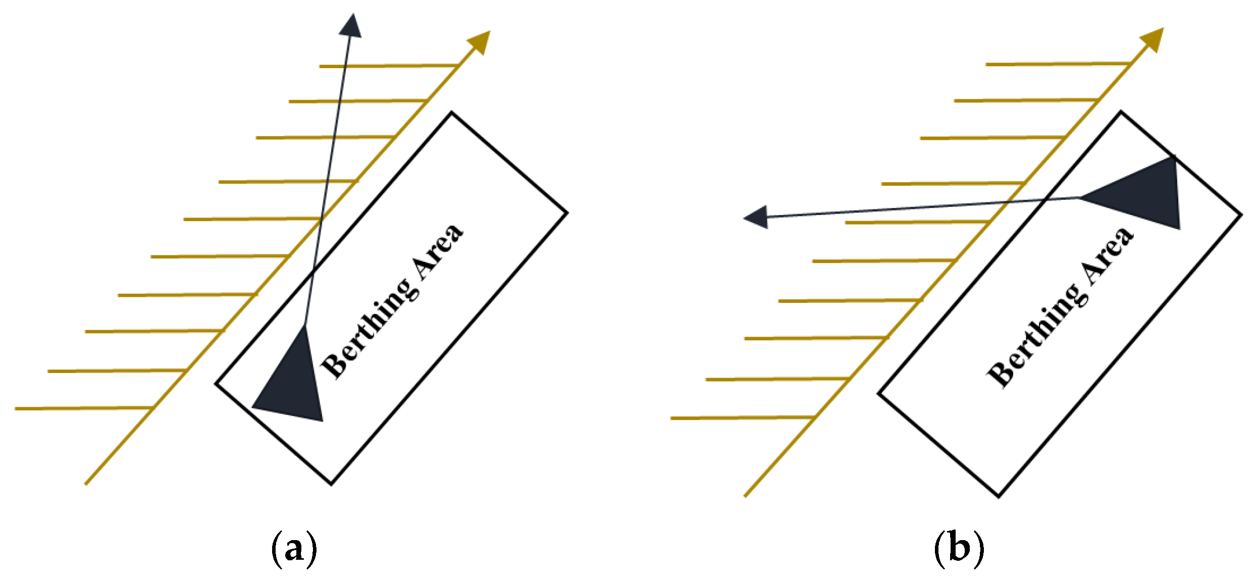
Considering the impact of vessel selection between downstream and upstream berthing modes on berthing route planning, the FM-DSB is proposed. This approach analyzes the relationship between water flow direction and berth position, combined with the berthing mode, to determine how the vessel enters the berth. Finally, the berthing path is planned using a two-stage Bezier curve. By splicing the two-stage Bezier curves, the vessel’s control system can better track the berthing path, while aligning the berthing operation more closely with practical operational habits.

(2)

Based on the response of the vessel to rudder angle and propeller rotation speed, the vessel model is initially identified. With the model identification results as a reference, the acceleration and deceleration characteristics of the vessel are analyzed. The process of vessel speed variation is then compared with the berthing distance, facilitating velocity matching of the berthing path to achieve temporal coupling.

(3)

Designing a dual-loop path tracking control system for ships using a sliding mode controller with strong adaptability to uncertainties in system structural parameters. This control system decomposes path tracking into a major-loop path-tracking controller and a minor-loop speed-heading tracking controller. Finally, based on the results of path planning, the feasibility and effectiveness of the berthing path are validated using the dual-loop path tracker.

The remainder of this paper is organized as follows: In Section 2, the influence of downstream and upstream berthing selection on berthing path planning is analyzed. Combining with Bezier curves, the FM-DSB is proposed. Section 3 focuses on model identification of vessels in a maritime simulator, obtaining vessel responses to the propeller and rudder inputs, thereby introducing the BPVM. In Section 4, a dual-loop path tracking control system for vessel berthing process is implemented using sliding mode control and PID control.

2. Flow Matching Double Section Bezier Berth Method

This paper aims to achieve breakthroughs in automatic berthing for both upstream and downstream approaches. Through an analysis of the relationship between a vessel’s heading and the direction of water flow, criteria for determining upstream and downstream berthing during automatic berthing operations are established. Building upon this analysis, and integrating two-stage Bezier curves, a novel berthing method termed the FM-DSB is proposed.

2.1. Double Section Bezier Curve

In the design of berthing paths, this paper employs a combination of first-order Bezier curves and third-order Bezier curves, which together form a single berthing route. A first-order Bezier curve is defined by two control points, $P_0$ and $P_1$, typically utilized for creating simple curve segments. Its characteristic lies in the coincidence of the curve’s starting and ending points with the first and last control points, respectively, while the shape of the curve is jointly determined by the positions and directions of these two control points. The mathematical expression of a first-order Bezier curve is a linear equation, as shown in Equation (1),

$$B(t)=(1-t)·P_0+t·P_1,\hspace{1em}0\le t\le 1$$

(1)

where $B(t)$ represents the coordinates of any point on the curve, with $t$ being the parameter ranging from $\left[0,1\right]$.

A third-order Bezier curve requires four control points $P_0$, $P_1$, $P_2$, and $P_3$ for determination. It is more flexible than a first-order Bezier curve, enabling the description of more intricate curve shapes. The defining characteristic of a third-order Bezier curve is its potential deviation from the control points at the starting and ending points, being influenced by all four control points. Consequently, it can achieve more complex curve paths. Its mathematical expression is a cubic equation, as illustrated in Equation (2).

$$B(t)={(1-t)}^3·P_0+3t{(1-t)}^2·P_1+3t^2(1-t)·P_2+t^3·P_3,\hspace{1em}0\le t\le 1$$

(2)

This paper divides the entire berthing process into two stages: the in-bound stage and the in-moor stage. These two stages are continuous in time and are demarcated by a pre-set leader point, typically determined based on experience and connected, respectively, by a third-order Bezier curve and a first-order Bezier curve. The main task of the in-bound stage is to guide the vessel from the entrance of the port to the leader point near the berth. The in-moor stage involves guiding the vessel from the leader point to the berth and safely mooring it. The key tasks in this stage include controlling the vessel’s speed and orientation to align the vessel’s body parallel to the port and gradually reduce speed within the permissible berthing range. As shown in Figure 2, the diagram depicts a dual-stage Bezier berthing trajectory, with the green line (Route1) representing the in-bound stage and the blue line (Route2) representing the in-moor stage, separated by a yellow triangular leader point. The brown circle denotes the control points of the third-order Bezier curve (Route1). As Route2 is a first-order Bezier curve, its control points, representing the starting and ending points, are not illustrated in this diagram. Ultimately, the vessel successfully enters the berthing area indicated by the red rectangle.

The advantage of using dual-stage Bezier curves lies in their ability to easily adjust the vessel’s approach during berthing. Considering the influence of water flow, vessels may need to switch between berthing downstream and upstream. Dual-stage Bezier curves allow for flexible adjustment of control point positions based on different water flow conditions and vessel operational requirements, thereby altering the shape of the berthing curve to accommodate specific berthing needs. This enhances the adaptability and flexibility of berthing operations. Additionally, the smoothness of these curves helps maintain the stability and safety of the vessel’s trajectory, ensuring that there are no abrupt changes or discontinuities during turning and positional adjustments, thus improving the accuracy and reliability of berthing operations.

2.2. Flow Matching Algorithm

The berthing method of a vessel is typically influenced by the direction of water flow and can generally be categorized into berthing downstream and berthing upstream. During berthing upstream, the propulsion from the vessel’s propellers directly impacts the blade surface of the rudder, resulting in better rudder effectiveness. Conversely, during berthing downstream, the water flow generated by the propellers has difficulty acting on the blade surface of the rudder, reducing its effectiveness. Improper maneuvering during this phase may lead to the vessel colliding with the dock. Therefore, large vessels primarily utilize berthing upstream for maneuvering, except in instances where environmental factors such as port area limitations and tidal wind directions necessitate the consideration of navigational safety and efficiency, thereby requiring unconventional berthing downstream.

Based on the relationship between the ship’s heading and the direction of water flow, this study determines the criteria for berthing scenarios downstream and upstream. The judgment process comprises two main steps: firstly, determining the shoreline direction based on the direction of water flow. As illustrated in Figure 3, the left blue line represents the direction of water flow, the inclined yellow line represents the shoreline, the horizontal yellow line represents the land area, and the black rectangle indicates the designated berthing area. Initially, the shoreline is assumed to be a directionless straight line. Then, this line is intersected with the direction of water flow, with the direction forming acute angles with the water flow being designated as the shoreline direction. Subsequently, the berthing direction is determined based on the shoreline direction and the berthing mode. As depicted in Figure 4a, if the berthing mode is downstream, the vessel’s heading upon completion of berthing should form an angle of less than 90° with the shoreline direction, as described by the angle relationship in Equation (3),

$$\left|\phi -{\phi }_{coast}\right|\le \frac{\pi }{2},\phi \in \left[0,2\pi \right),{\phi }_{coast}\in \left[0,2\pi \right)$$

(3)

where $\phi$ represents the ship’s heading, and ${\phi }_{coast}$ denotes the direction of the coastline.

In contrast, when the berthing mode, as illustrated in Figure 4b, is upstream berthing, the ship’s heading upon completion of berthing should form an angle greater than 90° but less than or equal to 180° with the coastline direction, as depicted in Equation (4).

$$\frac{\pi }{2}<\left|\phi -{\phi }_{coast}\right|\le \pi ,\phi \in \left[0,2\pi \right),{\phi }_{coast}\in \left[0,2\pi \right)$$

(4)

In summary, the pseudocode for the flow matching algorithm is presented in Algorithm 1.

Algorithm 1 Berthing Direction Determination

Input: Berthing method, Water flow direction, Coastline

Output: Berthing direction

1. Function Determine Berthing Direction (Berthing Method, Water Flow Direction, Coastline Direction)

2.   Initialize coastline direction as an undirected line.

3.   Determine acute angle between coastline and water flow direction.

4.   Set coastline direction to the direction of the acute angle.

5.   if Berthing Method is “Downstream Berthing” then

6.     Set the angle between vessel’s final heading and coastline direction <90°.

7.   End if

8.   if Berthing Method is “Upstream Berthing” then

9.     Set the angle between vessel’s final heading and coastline direction >90°and ≤ 180.

10.    End if

11. End Function

3. Berthing Path Velocity Matching Method

This paper aims to achieve the matching of berthing trajectory and speed by obtaining the vessel’s response curves through ship handling simulators and identifying the vessel model as a first-order linear model. Based on the identified model, the acceleration and deceleration characteristics of the vessel are analyzed by processing the response of the vessel’s propeller input to the vessel’s speed model, thus matching the berthing trajectory with the speed.

3.1. Three-Degree-of-Freedom Ship Model

Given that the center of gravity of a USV is located in the lower part of the vessel and horizontal motion is predominant in most cases, the influences of heave, pitch, and roll motions are negligible and can be disregarded in this paper. Therefore, the motion model of the USV in this paper is simplified into a three-degree-of-freedom (3-DOF) model covering sway, surge, and yaw [20]. The motion parameters for each DOF are listed in

Table 1. Motion parameters of vessel in 3DOF.

Motions/Rotations	Positions/Rotation Angles	Linear Velocities/ Angular Velocities	Forces/Moments
Surge	$x$	$u$	$X$
Sway	$y$	$v$	$Y$
Yaw	$\phi$	$r$	$N$

. Two coordinate systems are used to describe the motion of the USV (Figure 5): the space-fixed coordinate system $(O-X_0{Y}_0)$ and the body-fixed coordinate system $(o-x_0{y}_0)$. Additionally, the red rectangle in Figure 5 represents the USV. In these coordinate systems $x$, $y$, and $\phi$ represent the position and yaw angle of the USV; $u$, $v$, and $r$ denote the components of motion velocity and yaw velocity; and $U$ represents the resultant velocity of the vessel. Additionally, $X$, $Y$, and $N$ represent the external forces and moments acting on the hull; $\delta$ is the rudder angle; $\beta$ is the drift angle.

The linear equation representing the second-order linear response of the ship’s yaw velocity is shown in Equation (5),

$$T_1{T}_2\ddot{r}+(T_1+T_2)\dot{r}+r=K\delta +K{T}_3\dot{\delta }$$

(5)

where $T_1$, $T_2$ and $T_3$ represent the parameters of the equation.

In this paper, to facilitate the analysis of the ship’s yaw characteristics, the simplified first-order linear KT equation derived from NOMOTO [21], as presented in Equation (6), is adopted.

$$T\dot{r}+r=K\delta$$

(6)

The coefficients $K$ and $T$ carry distinct physical meanings: $K$ represents the turning ability index, reflecting the ship’s performance in terms of turning ability; $T$ stands for the rudder response index, indicating the response speed of yaw to steering. Equation (6) exhibits favorable performance in solving and analyzing heading-related issues, hence it has been widely applied.

This paper conducts an analysis of the response of ship speed to propeller input, considering that ship speed is not only influenced by the propeller rotation rate but also by the ship’s motion inertia. Therefore, taking the first-order KT model as a reference, the relationship between speed and propeller rotation speed is approximated as a first-order linear model, as shown by the specific expression in Equation (7).

$$T_u\dot{u}+u=K_u{n}_p$$

(7)

similarly, $K_u$ represents the acceleration performance index, indicating the quality of a vessel’s acceleration performance; $T_u$ stands for the propeller response index, indicating the speed at which the propeller responds to changes in ship speed. This study obtained responses of the ship to different inputs by conducting manipulation experiments with various rudder angles and speeds in a ship motion simulator. Subsequently, the ship’s motion model parameters were identified using the least squares identification algorithm [22]. The specific ship parameters used are listed in

Table 2. Ship physical parameters.

Subjects	Value
Length of ship, $L\left(\mathrm{m}\right)$	134
Breadth of ship, $B\left(\mathrm{m}\right)$	13
Depth of ship, $D\left(\mathrm{m}\right)$	9.8
Displacement, $\Delta {(\mathrm{m}}^3)$	6683
Draft of ship, $T\left(\mathrm{m}\right)$	4
Prismatic coefficient, $Cp$	0.651
Rudder deflection rate, $(\mathrm{deg}/\mathrm{s})$	2
Projected area of rudder, $A_r{(\mathrm{m}}^2)$	33.7999
No. of blades	5
Propeller diameter, $D\left(\mathrm{m}\right)$	3.944

. It is noteworthy that the ship model employed in this study is equipped with two propellers that share identical physical parameters. To facilitate the identification of the ship motion model, both propellers are set to maintain a consistent rotational speed throughout the research. By simultaneously rotating both propellers, the vessel is provided with powerful propulsion, enabling it to accelerate and decelerate quickly.

The response of the ship to the inputs of propeller and rudder angles is depicted in Figure 6 and Figure 7. In the manipulation experiments concerning the relationship between ship speed and propeller rotation speed, this study conducted experiments involving propeller rotation speed of $n_p=3\mathrm{rps}$ and $n_p=5\mathrm{rps}$ for forward propeller rotation, followed by experiments with propeller rotation speed of $n_p=-3\mathrm{rps}$ and $n_p=-5\mathrm{rps}$ for propeller reverse rotation. In Figure 6, the speed response curve clearly shows that the thrust exerted on the ship by forward and reverse propeller rotations is significantly different; the thrust exerted on the ship during propeller reverse rotation is only approximately 60% of that during forward rotation. Meanwhile, when identifying the relationship between propeller and ship speed, this study sets the rudder angle to 0 degrees. This practice leads to the model overlooking the deceleration effect of the rudder on the vessel, resulting in an overestimation of the ship’s acceleration performance compared to real-world scenarios. As a consequence, the vessel can reach maximum speed in a shorter time frame in this study than it would in reality.

The identified models of the yaw response system and the speed response system are represented by Equations (8) and (9), respectively.

$$29.172\dot{r}+r=10.644\delta$$

(8)

$$\left\{\begin{array}{l}21.899\dot{u}+u=2.5185n_p,\hspace{1em}{n}_p\in \left[0,5\mathrm{rps}\right]\\ 29.035\dot{u}+u=1.7244n_p,\hspace{1em}{n}_p\in \left[-5\mathrm{rps},0\right]\end{array}\right.$$

(9)

In this study, due to the focus of heading adjustments primarily during the in-bound phase, the surge velocity $u$ maintains a relatively high value during this stage. Conversely, during the in-moor phase, although the surge velocity $u$ decreases, it does not involve significant angular adjustments of heading because the main objective during this phase is speed reduction. Consequently, throughout the entire berthing task, the sway velocity $v$ remains within a relatively low range compared to the surge velocity $u$. Given these considerations, it can be assumed that Equation (10) holds during the berthing process. Therefore, the formula for updating the vessel’s position is as depicted in Equation (11).

$$U(t)=u(t)$$

(10)

$$\left\{\begin{array}{l}\dot{x}=U\cos \phi \\ \dot{y}=U\sin \phi \end{array}\right.$$

(11)

3.2. Velocity Matching Algorithm

Based on the response of the vessel’s speed to different propeller inputs shown in Figure 6 in the preceding section, it is evident that as the propeller rotation speed increases within a certain range, the vessel’s acceleration/deceleration response becomes faster, eventually stabilizing the speed at a fixed value. With the berthing route determined, to expedite the berthing process, the propeller control input should be maintained at a relatively high value. Therefore, in this study, when the vessel needs to accelerate, the propeller is set to a fixed higher forward rotation speed; whereas when the vessel needs to decrease its speed, the propeller is set to a fixed higher reverse rotation speed.

The BPVM proposed in this paper divides the control strategy of vessel berthing into two categories: “Acceleration-Constant Velocity-Deceleration” (ACD) and “Acceleration-Deceleration” (AD). The ACD strategy is suitable for longer berthing distances, allowing the vessel to accelerate from its initial speed to maximum speed with a fixed propeller rotation speed, maintain a constant speed for a period, and finally reduce speed by reversing the propeller to complete the berthing process. On the other hand, the AD strategy is applicable to tasks with shorter berthing distances, where it is challenging to complete the entire acceleration process due to the short distance between the starting and ending points. Before the vessel reaches the constant velocity stage, it has already reached the minimum deceleration distance at that speed, thus directly entering the deceleration phase.

The relationship between the ACD strategy and the AD strategy at various stages is illustrated in Figure 8. The blue curve represents the variation of vessel speed under the ACD strategy control, where $\left[0,t_1\right]$ denotes the acceleration stage, $[t_1,t_2]$ represents the constant velocity stage, and $[t_2,t_3]$ indicates the deceleration stage. The dashed pink line represents the propeller control input under the ACD strategy, maintaining $n_p=5\mathrm{rps}$ during $\left[0,t_2\right]$ and transitioning to $n_p=-5\mathrm{rps}$ during $\left[t_2,t_3\right]$. The red curve illustrates the vessel speed variation under the AD strategy control, with $\left[0,t_4\right]$ denoting the acceleration stage and $[t_4,t_5]$ representing the deceleration stage. Similarly, the propeller maintains $n_p=5\mathrm{rps}$ during $\left[0,t_4\right]$ and transitions to $n_p=-5\mathrm{rps}$ during $\left[t_4,t_5\right]$.

Although the velocity curves of both the ACD and AD strategies are composed of multiple segments, they share a common characteristic: the area they enclose with the coordinate axes represents the distance traveled by the vessel during the berthing process. The sum of the areas of each stage corresponds to the total length of the berthing path planned by the path planning module. Therefore, by analyzing the relationship between the distance and velocity curves, the start and end times of each stage can be determined, thereby locating key time points along the berthing path and achieving speed matching.

In the ACD strategy, when the initial velocity of the vessel $U_0$ and the propeller rotation speed $n_p$ are constant, according to the acceleration characteristics, the time $t_1$ required for the vessel to accelerate to the maximum velocity $U_{con}$ is a fixed value. Therefore, the distance $S_{acc}$ during the acceleration phase can be calculated by the integral formula shown in Equation (12). Similarly, based on the deceleration characteristics, the time required for the vessel to decelerate from the maximum velocity $U_{con}$ to $U=0 \mathrm{m}/\mathrm{s}$, denoted as $\left(t_3-t_2\right)$, is also a fixed value. Hence, the distance $S_{dcc}$ during the deceleration phase can be obtained through Equation (13). The $t_2$ mentioned above is the start time of the deceleration phase and is also the end time of the constant velocity phase. The $t_3$ represents the end time of the deceleration phase and is also the termination time of the berthing task. After determining $S_{acc}$ and $S_{dcc}$, according to the relationship between the total berthing distance $S_{all}$, $S_{acc}$ and $S_{dcc}$, as shown in Equation (14), the distance $S_{con}$ during the constant velocity phase can be obtained, thus determining the values of $t_2$ and $t_3$.

$$S_{acc}={\displaystyle {\int }_0^{t_1}U(t)dt}$$

(12)

$$S_{dcc}={\displaystyle {\int }_{t_2}^{t_3}U(t)dt}$$

(13)

$$S_{all}=S_{acc}+S_{con}+S_{dcc}$$

(14)

In the AD strategy, constrained by the berthing distance, the vessel’s velocity can only accelerate to $U_{acc2}$. Therefore, it is necessary to adjust the duration of the acceleration phase, denoted as $t_4$, to ensure that both the distances $S_{acc2}$ and $S_{dcc2}$ during the acceleration and deceleration phases, respectively, meet the requirement outlined in Equation (15), where $\xi$ represents the predetermined error threshold. In summary, the pseudocode for velocity matching is provided in Algorithm 2. Here, $\xi$ denotes the increment threshold for $U_{acc2}$.

$$\left|S_{all}-S_{acc2}-S_{dcc2}\right|<\xi$$

(15)

Algorithm 2 Velocity Matching Method

Input: Navigation path planning results

Output: Duration of each stage in the berthing process

1. Function Determine Berthing Process (Path Planning Result)

2.  Obtain the total length of the berthing path $S_{all}$ based on the path planning module.

3.  Calculate the time $t_1$ and distance $S_{acc}$ to accelerate to a constant velocity $U_{con}$ based on the acceleration characteristics curve.

4.  Determine the deceleration distance $S_{dcc}$ and the duration $\left(t_3-t_2\right)$ to decelerate from velocity $U_{con}$ to 0 based on the deceleration characteristics curve.

5.  Calculate the distance of the constant velocity stage $S_{con}=S_{all}-S_{acc}-S_{dcc}$, and thus determine the duration of the constant velocity stage $\left(t_2-t_1\right)$, and obtain the end times $t_2$ and $t_3$ for the constant velocity and deceleration stages, respectively.

6.    $\mathbf{If} t_1\ge t_2$ then

7.    Skip the constant velocity stage, and the berthing process consists only of the acceleration and deceleration stages, where the maximum velocity during acceleration will not reach the constant velocity $U_{con}$.

8.    Set the velocity $U_{acc2}$ to 0.

9.    Increment $U_{acc2}$ to $U_{acc2}+\epsilon$.

10.     Determine the stop time t4 for acceleration and the stop time $t_5$ for deceleration, along with the distances ${\mathrm{S}}_{acc2}$ and ${\mathrm{S}}_{dcc2}$.

11.    $\mathrm{If} \left(S_{all}-S_{acc}-S_{dcc}\right)<\xi$ then

12.      Output $t_4$ and $t_5$.

13.      Jump to line 20.

14.     Else

15.      Jump to line 9.

16.     End if

17.  Else

18.     End the function and output $t_1$, $t_2$, and $t_3$

19.  End if

20. End Function

4. Dual-Loop Path Tracking Control System

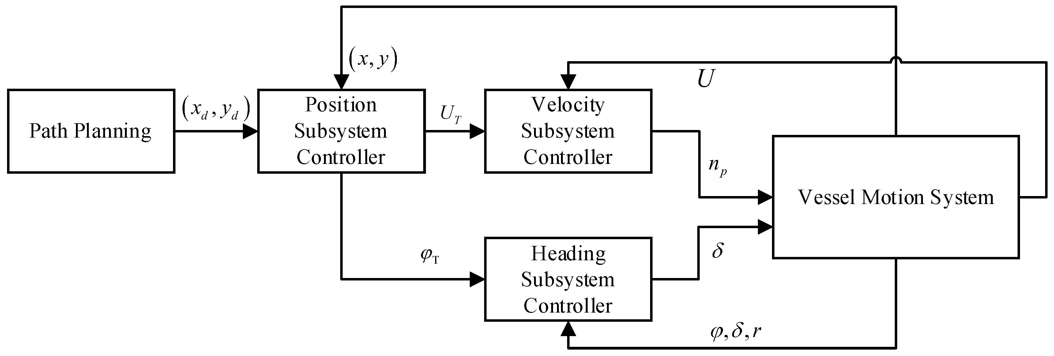
This paper presents a dual-loop path-tracking control system for tracking the position, velocity, and heading of a vessel. The control system diagram is shown in Figure 9. The outer loop consists of the position tracking subsystem, while the inner loop consists of the velocity and heading tracking subsystems. The outer loop obtains the desired position $\left(x_d,y_d\right)$ from the path planning module and generates intermediate command targets for velocity $U_T$ and heading ${\phi }_T$. After the heading tracking subsystem in the inner loop obtains the target heading ${\phi }_T$, it generates the rudder angle change control command $\dot{\delta }$ using the sliding mode control to track the heading. After the velocity tracking subsystem in the inner loop obtains the desired velocity $U_T$, it generates propeller control commands $n_p$ through PD control to track and control the velocity $U$.

The kinematic model of the vessel can be derived from Equations (6), (7), (10) and (11).

$$\left\{\begin{array}{l}\begin{array}{l}\dot{x}=U\cos \phi \hfill \\ \dot{y}=U\sin \phi \hfill \\ \dot{\phi }=r\hfill \\ \dot{r}=\frac{K\delta -r}{T}\hfill \\ \dot{U}=\frac{K_u{n}_p-U}{T_u}\hfill \end{array}\hfill \end{array}\right.$$

(16)

4.1. Position Tracking Control Subsystem

The position tracking control subsystem achieves the tracking of $(x,y)$ to $(x_d,y_d)$ solely by obtaining the desired position $(x_d,y_d)$ and designing a sliding mode control law. Equation (16) can be simplified to Equation (11):

Let:

$$\left\{\begin{array}{l}U\cos \phi =u_1\\ U\sin \phi =u_2\end{array}\right.$$

(17)

The tracking error equations are given by Equation (18):

$$\left\{\begin{array}{l}{\dot{x}}_e=u_1-{\dot{x}}_d\\ {\dot{y}}_e=u_2-{\dot{y}}_d\end{array}\right.$$

(18)

The sliding surfaces $s_1$ and $s_2$ are designed as shown in Equation (19):

$$\left\{\begin{array}{l}{s}_1=x_e\\ s_2=y_e\end{array}\right.$$

(19)

Then, from Equations (18) and (19):

$$\left\{\begin{array}{l}{\dot{s}}_1={\dot{x}}_e=u_1-{\dot{x}}_d\\ {\dot{s}}_2={\dot{y}}_e=u_2-{\dot{y}}_d\end{array}\right.$$

(20)

The control laws $u_1$ and $u_2$ are designed as shown in Equation (20):

$$\left\{\begin{array}{l}{u}_1={\dot{x}}_d-k_1{s}_1,k_1>0\\ u_2={\dot{y}}_d-k_2{s}_2,k_2>0\end{array}\right.$$

(21)

Convergence analysis of the sliding surfaces $s_1$ and $s_2$: Define a Lyapunov candidate function as shown in Equation (22):

$$V=\frac{1}{2}{s}_1{ }^2$$

(22)

Taking the derivative of Equation (22):

$$\dot{V}=s_1{\dot{s}}_1$$

(23)

From Equations (20) and (21):

$${\dot{s}}_1=-k_1{s}_1$$

(24)

Substituting Equation (24) into Equation (23):

$$\dot{V}=s_1{\dot{s}}_1=-k_1{s}_1{ }^2=-2k_{1}V$$

(25)

Therefore, the sliding surface $s_1$ converges to 0. Similarly, it can be proven that $s_2$ also converges to 0, which leads to the convergence of $(x,y)$ to $(x_d,y_d)$.

When the control laws in the ideal trajectory control law of Equation (21) can be achieved, the values of $U$ and $\phi$ in Equation (17) correspond to the desired values of $U_T$ and ${\phi }_T$ for the ideal trajectory, and thus expressions for $U_d$ and ${\phi }_d$ can be derived as shown in Equation (26):

$$\left\{\begin{array}{l}{\phi }_T=\arctan \frac{u_2}{u_1}\\ U_T=\frac{u_1}{\cos {\phi }_T}\end{array}\right.$$

(26)

4.2. Heading Tracking Control Subsystem

The heading tracking control subsystem reduces the error between the heading angle $\phi$ and the target heading angle ${\phi }_T$ by designing a sliding mode controller to control the rate of change of the rudder angle $\dot{\delta }$.

The variables are defined as follows:

$$\left\{\begin{array}{l}{x}_1=\phi \\ x_2=r\\ x_3=\delta \\ x_d={\phi }_d\end{array}\right.$$

(27)

Taking the derivative of Equation (27):

$$\left\{\begin{array}{l}{\dot{x}}_1=x_2\\ {\dot{x}}_2=\frac{-x_2+K{x}_3}{T}\\ {\dot{x}}_3=\dot{\delta }\end{array}\right.$$

(28)

The error equations are defined as:

$$\left\{\begin{array}{l}{e}_1=x_1-x_d\\ e_2={\dot{e}}_1=x_2-{\dot{x}}_d\\ e_3={\dot{e}}_2=-\frac{1}{T}{x}_2+\frac{K}{T}{x}_3-{\ddot{x}}_d\end{array}\right.$$

(29)

The sliding surface is defined as:

$$s_3=c_1{e}_1+c_2{e}_2+e_3,c_i>0,i=1,2$$

(30)

The sliding mode reaching law is defined as:

$${\dot{s}}_3=-M\mathrm{sgn}\left(s_3\right)-\lambda s_3,M>0,\lambda >0$$

(31)

Combining Equations (30) and (31), the sliding mode control law is derived as:

$$\dot{\delta }=\frac{T}{K}\left(-M\mathrm{sgn}\left(s_3\right)-\lambda s_3+P{x}_2+Q{x}_3\right)$$

(32)

where $P=-\frac{1}{T}\left(c_{1}T-c_2+\frac{1}{T}\right)$, $Q=\frac{K}{T}\left(\frac{1}{T}-c_2\right)$.

Convergence analysis of the sliding surface $s_3$: Define a Lyapunov candidate function as:

$$V=\frac{1}{2}{s}_3{ }^2$$

(33)

Taking the derivative of Equation (33):

$$\dot{V}=s_3{\dot{s}}_{{ }_3}$$

(34)

From Equations (33) and (34):

$$\dot{V}=-s_{3}M\mathrm{sgn}\left(s_3\right)-\lambda s_3{ }^2\le 0$$

(35)

Therefore, the sliding surface $s_3$ converges to 0, which leads to the convergence of $\phi$ to ${\phi }_T$.

4.3. Velocity Tracking Control Subsystem

The task of the velocity tracking control system is to track the desired velocity $U_T$ quickly and accurately. In this paper, a PD controller is chosen for velocity tracking control.

The velocity tracking error is defined as:

$$U_e=U_T-U$$

(36)

Then, the desired velocity tracking PD control law is given by:

$$n_p\left(k+1\right)=K_p{U}_e\left(k+1\right)+K_D\left(U_e\left(k+1\right)-U_e\left(k\right)\right)$$

(37)

where $K_p$ is the proportional coefficient and $K_D$ is the derivative coefficient.

5. Results and Discussion

In this chapter, experiments were conducted on both long-distance and short-distance berthing to validate the effectiveness of the path-planning algorithm based on FM-DSB and BPVM. Based on the planning results, the feasibility and effectiveness of the berthing path were verified using a dual-loop path tracker.

The vessel parameters utilized in the simulation experiments are shown in Table 2. The identified vessel motion model is depicted by Equation (38), with the parameters therein listed in

Table 3. Vessel motion model parameters.

Subjects	Value	Subjects	Value
$K_1$	29.172	$T$	10.644
$K_2$	21.899	$T_1$	2.5185
$K_3$	29.035	$T_2$	1.7244

.

$$\left\{\begin{array}{l}\begin{array}{c}\dot{x}=U\cos \phi \hfill \\ \dot{y}=U\sin \phi \hfill \\ \dot{\phi }=r\hfill \\ \dot{r}=\frac{K_1\delta -r}{T_1}\hfill \\ \begin{array}{l}\dot{U}=\frac{K_2{n}_p-U}{T_{{ }_2}},n_p>0\\ \dot{U}=\frac{K_3{n}_p-U}{T_3},n_p<0\end{array}\hfill \end{array}\hfill \end{array}\right.$$

(38)

In the experiment, the range of vessel motion parameters was restricted. These motion state parameters are described by Equation (39), while the control parameters are defined by Equation (40).

$$\left\{\begin{array}{l}0\le U\le 12.49\left(\mathrm{m}/\mathrm{s}\right)\\ -\frac{15}{180}\pi \left(\mathrm{rad}/\mathrm{s}\right)\le r\le \frac{15}{180}\pi \left(\mathrm{rad}/\mathrm{s}\right)\\ 0\le x\le 3000\left(\mathrm{m}\right)\\ 0\le y\le 3000\left(\mathrm{m}\right)\\ 0\le \phi <2\pi \left(\mathrm{rad}\right)\\ -\frac{30}{180}\pi \left(\mathrm{rad}\right)\le \delta \le \frac{30}{180}\pi \left(\mathrm{rad}\right)\end{array}\right.$$

(39)

$$\left\{\begin{array}{l}-5\left(\mathrm{rps}\right)\le n_p\le 5\left(\mathrm{rps}\right)\\ -\frac{5}{180}\pi \left(\mathrm{rad}/\mathrm{s}\right)\le \dot{\delta }\le \frac{5}{180}\pi \left(\mathrm{rad}/\mathrm{s}\right)\end{array}\right.$$

(40)

In the experiment, when the vessel’s state simultaneously meets the following three conditions, it is considered that the vessel has completed the berthing task.

(1)

The vessel sails into the rectangular berth area centered around the endpoint (EP), satisfying the positional parameter requirements specified by Equation (41).

(2)

The vessel’s hull aligns approximately parallel to the berth while maintaining stability, indicating that the heading angle $\phi$ and yaw velocity $r$ meet the requirements specified by Equation (42), where ${\phi }_p$ represents the berth angle.

(3)

The vessel’s speed meets the berthing conditions, meaning that the vessel’s speed satisfies the requirements specified by Equation (43).

$$\left\{\begin{array}{l}EP(1)-5\left(\mathrm{m}\right)\le x\le EP(1)+5\left(\mathrm{m}\right)\\ EP(2)-5\left(\mathrm{m}\right)\le y\le EP(2)+5\left(\mathrm{m}\right)\end{array}\right.$$

(41)

$$\left\{\begin{array}{l}-\frac{1}{12}\pi \left(\mathrm{rad}\right)\le \phi -{\phi }_p\le \frac{1}{12}\pi \left(\mathrm{rad}\right)\\ -\frac{1}{180}\pi \left(\mathrm{rad}/\mathrm{s}\right)\le r\le \frac{1}{180}\pi \left(\mathrm{rad}/\mathrm{s}\right)\end{array}\right.$$

(42)

$$\left\{\begin{array}{l}-5\left(\mathrm{rps}\right)\le n_p\le 5\left(\mathrm{rps}\right)\\ -\frac{5}{180}\pi \left(\mathrm{rad}/\mathrm{s}\right)\le \dot{\delta }\le \frac{5}{180}\pi \left(\mathrm{rad}/\mathrm{s}\right)\end{array}\right.$$

(43)

The experiment is conducted using MATLAB R2023b on a desktop with a 48 GB DDR4 RAM, an AMD Ryzen 7 5800X 3.80 GHz CPU (Sunnyvale, CA, USA), a GeForce RTX 3080 GPU (NVIDIA, Santa Clara, CA, USA), and a 1 TB SSD hard drive.

5.1. Long-Distance Berthing Experiment

In this experimental section, the simulation environment is configured for a long-distance scenario. By designing the scene parameters, the berthing process of the vessel conforms to the motion process of “Acceleration-Constant Speed-Deceleration”. The start point is $Sp=\left[0,0\right]$ and the berth end point is $Ep=\left[2000 \mathrm{m},1100 \mathrm{m}\right]$. The initial heading is ${\phi }_0=0$. The direction of water flow is ${\phi }_w=\frac{\pi }{2}$. Based on the water flow direction, the BPVM method can calculate the direction of the coastline as ${\phi }_{coast}=\frac{\pi }{2}$. The control point for the in-bound stage of the Bezier curve is set to $\left[p_1,p_2,p_3,p_4\right]$, and the control point for the in-moor stage is set to $\left[p_4,p_5\right]$. The expression for the control points is shown in Equation (44). 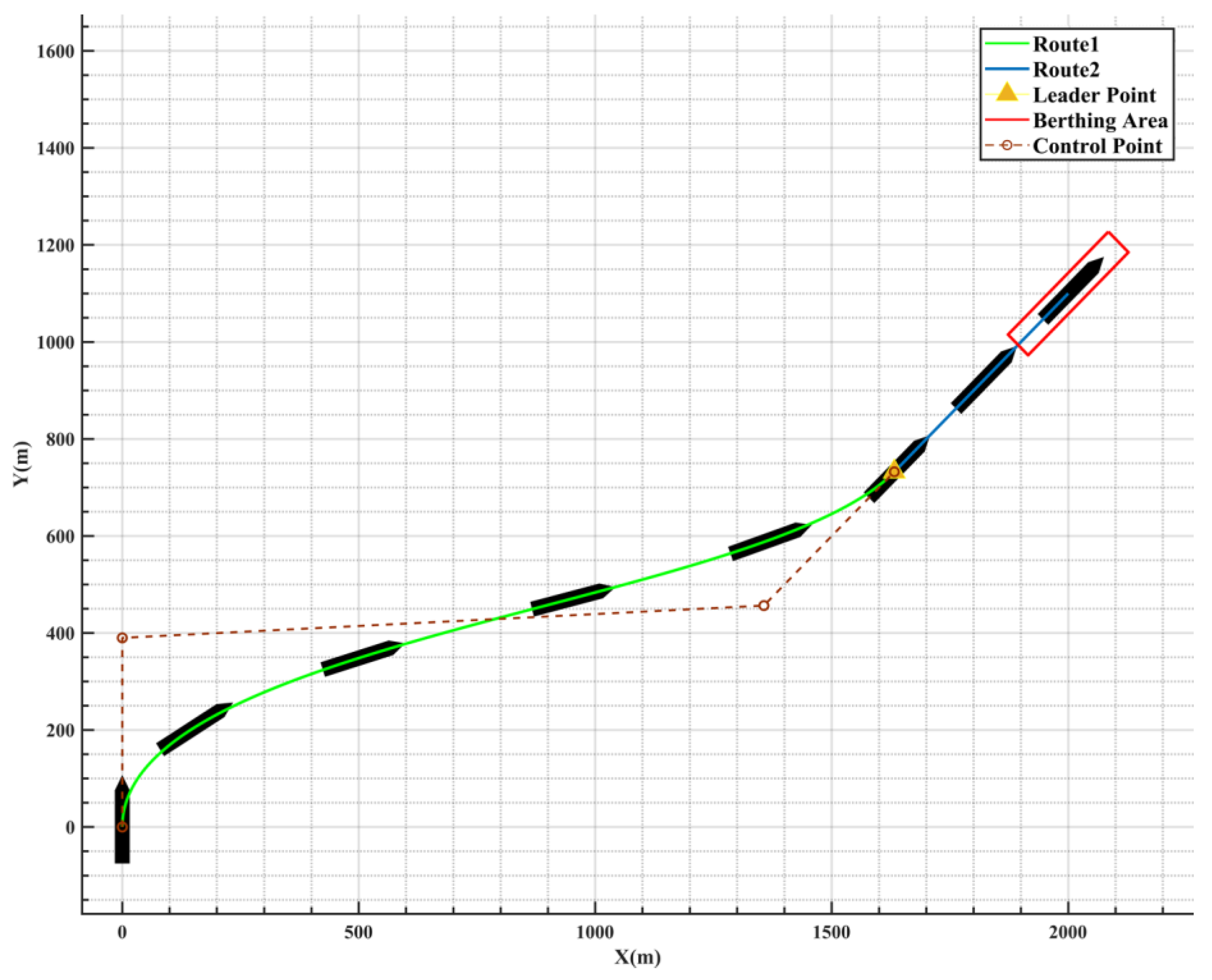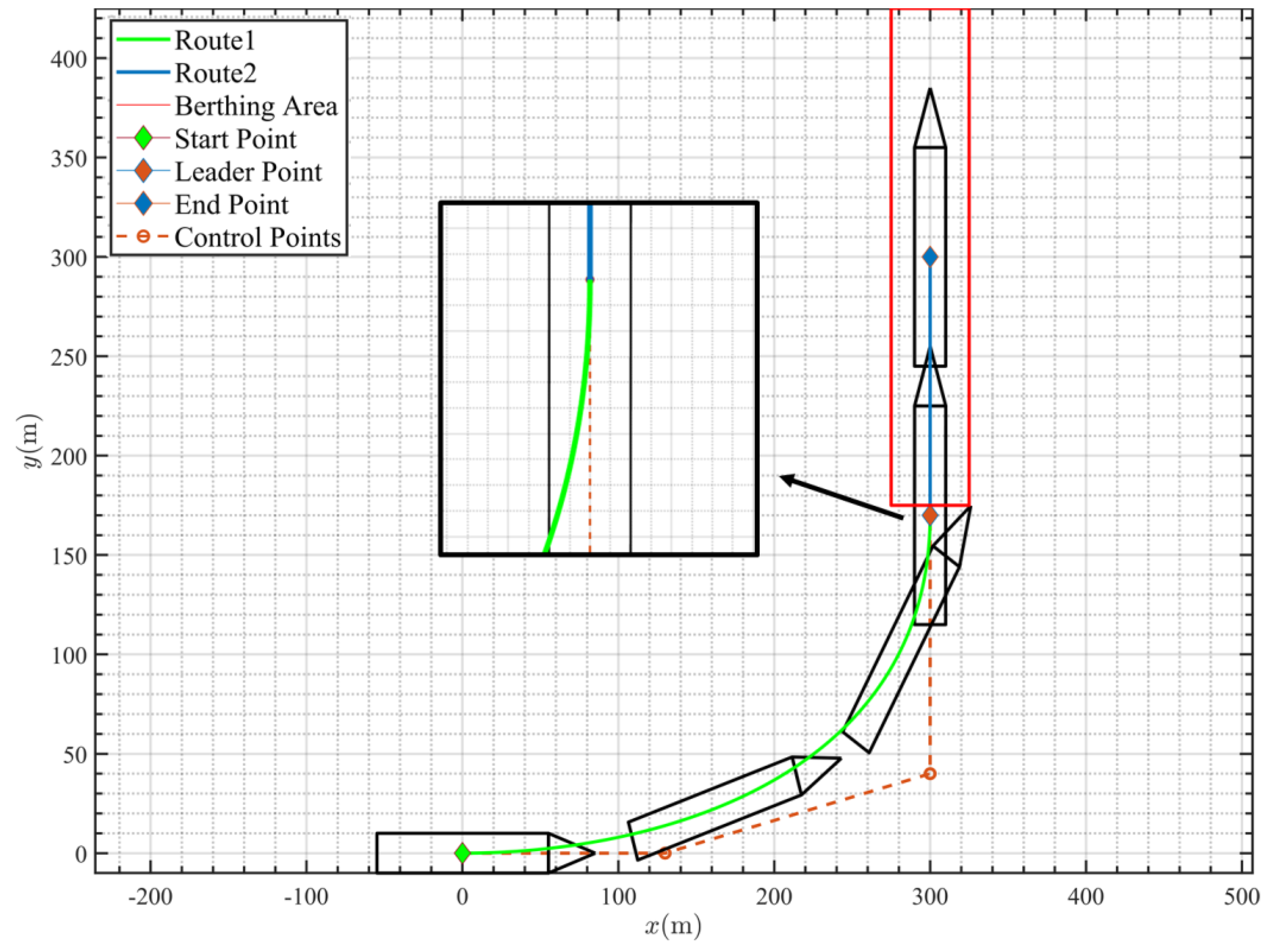Among these points, point $p_1$ represents the start point, point $p_2$ is a point extended along the initial heading by three times the ship’s length, point $p_5$ is the berthing endpoint, point $p_4$ is determined by extending the berthing stopping heading backwards by four times the ship’s length from the endpoint, and point $p_3$ is determined by extending the berthing stopping heading backwards by seven times the ship’s length from the endpoint. The upstream berthing path is depicted in Figure 10, while the downstream berthing path is shown in Figure 11. The green curve (Route1) represents the in-bound stage berthing curve fitted with a third-order Bezier curve, while the red curve (Route2) represents the in-moor stage berthing curve fitted with a first-order Bezier curve. The red diamond marks the junction between the two Bezier segments, the green diamond represents the starting point, the blue diamond indicates the berthing endpoint, and the red dashed line represents the control points connecting the in-bound stage Bezier berthing curve. Since the slopes at the endpoints of third-order Bezier curves are equal to the slopes of the lines connecting the most adjacent control points, ensuring smoothness at the intersection of two Bezier curves can be achieved by adjusting the control point slopes of the third-order Bezier curve. The junction in Figure 10 and Figure 11 is magnified to facilitate the observation of the smoothness of the connection points of the two-segment Bezier curves. BPVM method is utilized to perform velocity matching on the berthing path. The matched results are shown in Figure 12. The blue curve and the green curve represent the velocity change curves for downstream berthing and upstream berthing, respectively, while the pink and orange dashed lines depict the corresponding propeller rotation speed curves for the berthing processes. According to Figure 12, the acceleration process of downstream berthing and upstream berthing is the same. At $t_1=106.5 \mathrm{s}$, they reach the maximum speed $U_{con}=12.49 \mathrm{m}/\mathrm{s}$. However, due to the longer distance for upstream berthing, the duration of the constant phase is longer. At $t_2=261.5 \mathrm{s}$, upstream berthing enters the deceleration stage. At this moment, the propeller rotation speed is adjusted to $n_p=-5\mathrm{rps}$, and the berthing task concludes at $t_3=287.8 \mathrm{s}$. Meanwhile, downstream berthing adjusts the propeller rotation speed to $n_p=-5\mathrm{rps}$ at $t_4=220.6 \mathrm{s}$ and enters the deceleration stage, ultimately concluding the berthing task at $t_5=246.8 \mathrm{s}$.

$$\left\{\begin{array}{l}{p}_1=\left[Sp\left(1\right),Sp\left(2\right)\right]\\ p_2=\left[Sp\left(1\right)+3L\cos \left({\phi }_0\right),Sp(2)+3L\sin \left({\phi }_0\right)\right]\\ p_3=\left[Ep\left(1\right)-7L\cos \left({\phi }_f\right),Sp(2)-7L\sin \left({\phi }_f\right)\right]\\ p_4=\left[Ep\left(1\right)-4L\cos \left({\phi }_f\right),Sp(2)-4L\sin \left({\phi }_f\right)\right]\\ p_5=\left[Ep\left(1\right),Ep\left(2\right)\right]\end{array}\right.$$

(44)

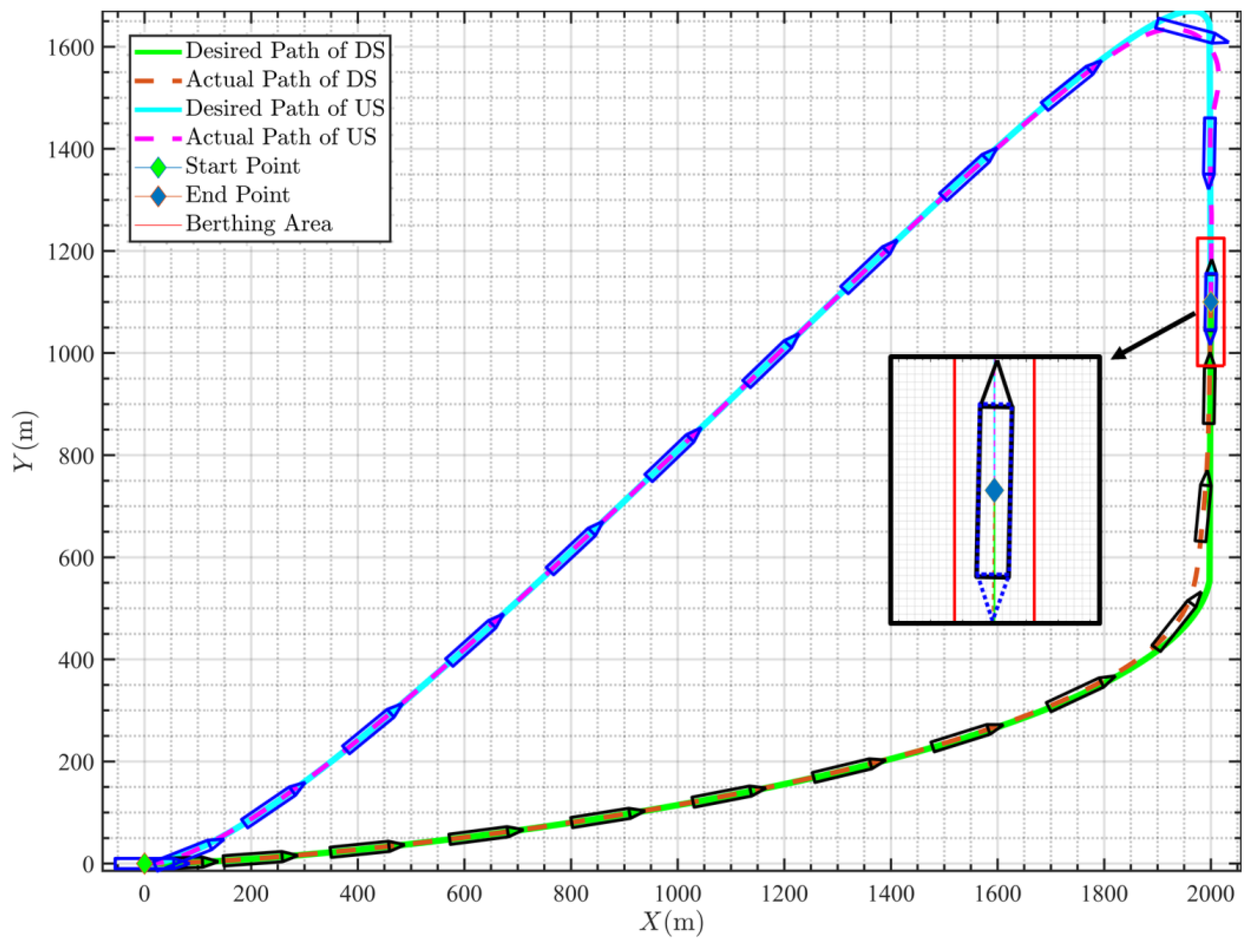
After obtaining the berthing path and matching velocity, the dual-loop path control system is utilized to track the desired path. The control system parameters are shown in

Table 4. The controller parameters for the long-distance berthing experiment.

Subjects	Value	Subjects	Value
$k_1$	0.12	$k_2$	0.12
$K_P$	5	$K_D$	0.01
$c_1$	0.1	$c_2$	0.5
$\lambda$	0.05	$M$	0.01

. The path-tracking performance is shown in Figure 13. The solid green and cyan lines, respectively, represent the desired paths $\left(X_d,Y_d\right)$ for downstream and upstream berthing, while the dashed red and pink lines depict the actual berthing curve $\left(X_a,Y_a\right)$ obtained from the simulation. Comparing the two curves, it can be observed that the dual-loop path tracking control system effectively tracked the target path and successfully completed the berthing task. To clearly observe the vessel’s attitude at the end of berthing, the endpoint position is magnified, as shown in Figure 13. From the magnified section, it can be observed that at the termination of the berthing task, the ship’s hull is nearly parallel to the berth, with the ship’s center positioned near the endpoint. For a clearer observation of the tracking effectiveness of the dual-loop tracking control system, Figure 14 displays the temporal tracking graph of the position, it can be observed from the graph that despite some temporal delay in position tracking, at the conclusion of the berthing task, the vessel’s position $\left(X_a,Y_a\right)$ closely aligns with the desired position $\left(X_d,Y_d\right)$.

The tracking performance of the vessel’s velocity is illustrated in Figure 15. The green and pink dashed lines, respectively, represent the desired velocity $U_d$ output by the BPVM method for downstream and upstream berthing. The red and blue solid lines represent the target velocity output by the position tracking subsystem. The cyan and black solid lines represent the actual vessel’s velocity curves. The yellow and purple solid lines represent the propeller rotation speed during the downstream and upstream berthing processes, respectively. From the graph, it can be observed that despite some oscillation in propeller rotation speed during the acceleration and deceleration phases, the velocity variation curve remains smooth. However, during the constant velocity phase, there exists a certain static deviation between the actual velocity $U_a$ and desired velocity $U_d$. This is attributed to the absence of an integral component in the design of the velocity controller, preventing error accumulation and resulting in a static speed deviation. 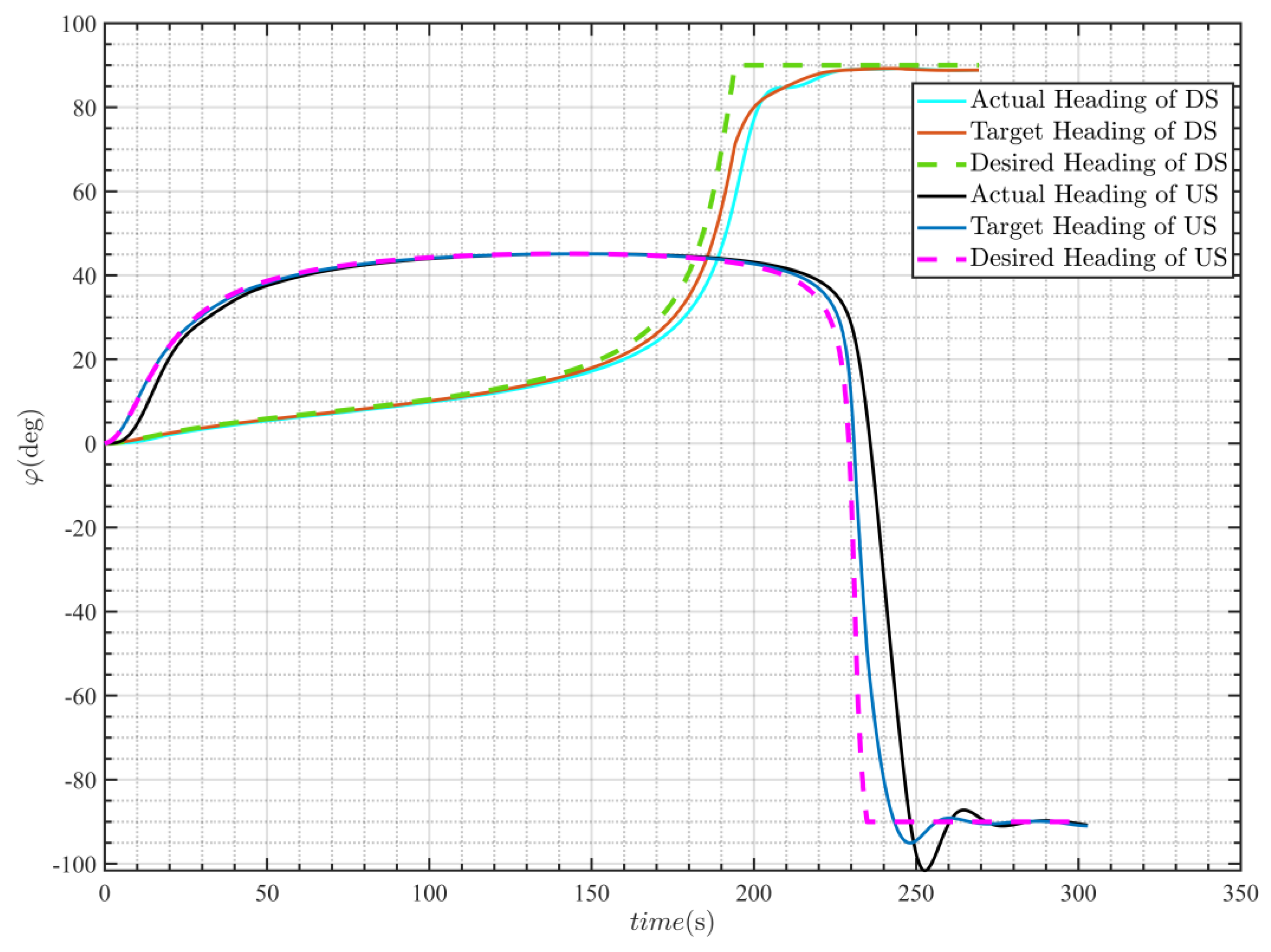Nonetheless, this is intentional within this study, as maintaining the desired position (X_d, Y_d) ahead of the vessel’s position $\left(X_a,Y_a\right)$ throughout the berthing task is advantageous for the stability of the control system. Similarly, the comparison between the desired heading ${\phi }_d$, target heading ${\phi }_T$, and actual heading ${\phi }_a$ is illustrated in Figure 16. The temporal variation curves of rudder angle $\delta$ and yaw velocity $r$ for downstream and upstream berthing are shown in Figure 17. From Figure 16 and Figure 17, it can be inferred that upon completing the final berthing task, the vessel’s heading aligns closely with the berth, with the rudder angle and yaw velocity essentially at 0. This indicates that immediately after the conclusion of the berthing task, the vessel’s heading remains relatively stable without significant changes.

5.2. Short-Distance Berthing Experiment

In this experimental section, the simulation environment was configured for a short-distance scenario. By designing the scenario parameters, the berthing process of the vessel conforms to an “Acceleration-Deceleration” motion sequence. The starting point coordinates were set as $Sp=\left[0,0\right]$, and the berth endpoint coordinates were defined as $Ep=\left[300 \mathrm{m},300 \mathrm{m}\right]$. The water flow direction was set as ${\phi }_w=\frac{\pi }{2}$. Based on this flow direction, the BPVM algorithm determined the coastline direction as ${\phi }_{coast}=\frac{\pi }{2}$. During downstream berthing, the heading of the vessel entering the berth was set as ${\phi }_f=\frac{\pi }{2}$, while during upstream berthing, the heading of the vessel entering the berth should be ${\phi }_f=-\frac{\pi }{2}$.

In a short-distance scenario, where the starting point and the endpoint are relatively close, adjustments were made to the initial headings and Bezier curve control points for downstream and upstream berthing experiments to ensure the smooth completion of the berthing task. This was performed to avoid potential challenges arising from the physical limitations of unmanned vessels, which may hinder effective tracking of the desired trajectory when curvature becomes excessive. In the upstream berthing scenario, as depicted in Figure 18, the vessel’s initial heading is set to ${\phi }_0=\frac{\pi }{2}$, with the control point equation given by Equation (45). Conversely, in the downstream berthing scenario, illustrated in Figure 19, the vessel’s initial heading is ${\phi }_0=0$, and the control point equation remains consistent with Equation (46). Similar to the method used for setting control points in the previous section, the control points for short-distance berthing in this section are also determined based on the initial and final headings, with a certain distance equivalent to the ship’s length. Additionally, the junction in Figure 18 and Figure 19 has also been magnified in the figures to facilitate the observation of the smoothness of the connection points of the two-segment Bezier curves.

$$\left\{\begin{array}{l}{p}_1=\left[Sp\left(1\right),Sp\left(2\right)\right]\\ p_2=\left[Sp\left(1\right)+5L\cos \left({\phi }_0\right),Sp(2)+5L\sin \left({\phi }_0\right)\right]\\ p_3=\left[Ep\left(1\right)-2L\cos \left({\phi }_f\right),Sp(2)-2L\sin \left({\phi }_f\right)\right]\\ p_4=\left[Ep\left(1\right)-L\cos \left({\phi }_f\right),Sp(2)-L\sin \left({\phi }_f\right)\right]\\ p_5=\left[Ep\left(1\right),Ep\left(2\right)\right]\end{array}\right.$$

(45)

$$\left\{\begin{array}{l}{p}_1=\left[Sp\left(1\right),Sp\left(2\right)\right]\\ p_2=\left[Sp\left(1\right)+L\cos \left({\phi }_0\right),Sp(2)+L\sin \left({\phi }_0\right)\right]\\ p_3=\left[Ep\left(1\right)-2L\cos \left({\phi }_f\right),Sp(2)-2L\sin \left({\phi }_f\right)\right]\\ p_4=\left[Ep\left(1\right)-L\cos \left({\phi }_f\right),Sp(2)-L\sin \left({\phi }_f\right)\right]\\ p_5=\left[Ep\left(1\right),Ep\left(2\right)\right]\end{array}\right.$$

(46)

Similar to the long-distance berthing experiment, the velocity profile after matching is illustrated in Figure 20. In downstream berthing, the vessel accelerates at a propeller rotation speed of $n_p=5\mathrm{rps}$ until $t_3=67.3 \mathrm{s}$, after which the propeller rotation speed is adjusted to $n_p=-5\mathrm{rps}$ to initiate the deceleration phase. The downstream berthing task concludes at $t_4=92.3 \mathrm{s}$ In upstream berthing, the vessel accelerates at a propeller rotation speed of $n_p=5\mathrm{rps}$ until $t_1=77.8 \mathrm{s}$, following which the propeller rotation speed is adjusted to $n_p=-5\mathrm{rps}$. Finally, the upstream berthing task concludes at $t_2=103 \mathrm{s}$.

Similar to the previous section, after obtaining the berthing path and matched velocities for short distances, the dual-loop path tracking control system was utilized to track the desired trajectory. The parameters of the control system are outlined in

Table 5. The controller parameters for the short-distance berthing experiment.

Subjects	Value	Subjects	Value
$k_1$	0.2	$k_2$	0.2
$K_P$	5	$K_D$	0.01
$c_1$	0.6	$c_2$	1.1
$\lambda$	0.8	$M$	0.001

. The path-tracking performance for close-range berthing is illustrated in Figure 21. From the graph, it can be observed that even in short-distance berthing scenarios, the dual-loop path control system is capable of effectively tracking the desired position $\left(X_d,Y_d\right)$. Even in locations with smaller turning radii, the system manages to guide the vessel along the expected path, and at the conclusion of the berthing task, the vessel’s heading is essentially parallel to the berth. Figure 22 depicts the temporal tracking graph of the vessel’s position, while Figure 23 presents the temporal tracking graph of the vessel’s heading. Figure 24 showcases the tracking performance of the vessel’s speed and the control input of the propeller rotation speed during the berthing process. From the graph, it is evident that there remains a certain static deviation between the actual velocity $U_a$ and the desired velocity $U_d$. Additionally, during the deceleration phase, the propeller rotation velocity does not maintain a constant $-5rps$ but gradually transitions from around $+5rps$ to $-5rps$. This results in a longer duration for the vessel to decelerate in the actual scenario. Finally, Figure 25 displays the temporal variation curves of the rudder angle and yaw velocity.

5.3. Discussion

In the first two sections of this chapter, experiments were conducted on both short-distance and long-distance berthing experiments. The experimental findings demonstrate that, concerning path planning, analysis of the vessel’s adherence to the desired trajectory in Figure 13 and Figure 21 reveals the effectiveness of the FM-DSB algorithm proposed herein, not only in facilitating berth path planning but also in ensuring the smooth and traceable nature of the paths. In terms of velocity planning during the berthing process, examination of the vessel’s propeller and speed response curves in Figure 15 and Figure 24 reveals that the BPVM algorithm proposed in this paper can effectively plan the vessel’s velocity, enabling it to accomplish the berthing task quickly and efficiently. In contrast to velocity planning algorithms based on empirical [5,23] or residual distance [1,6] methods, the proposed BPVM algorithm in this paper is tailored to better align with the acceleration and deceleration traits of vessels. The ability to adjust the propeller to negative thrust facilitates quicker berthing. Additionally, the devised berthing algorithm BPVM and FM-DSB demonstrate exceptional real-time performance. As shown in

Table 6. Time consumption of BPVM and FM-DSB algorithm in different berthing scenarios.

	Long-Distance (s)		Short-Distance (s)
Index	Upstream	Downstream	Upstream	Downstream
1	0.049	0.033	0.041	0.034
2	0.037	0.034	0.04	0.037
3	0.038	0.035	0.035	0.039
4	0.035	0.032	0.035	0.038
5	0.042	0.04	0.044	0.042
6	0.044	0.039	0.044	0.045
7	0.04	0.038	0.041	0.047
8	0.038	0.04	0.049	0.047
9	0.043	0.04	0.048	0.047
10	0.038	0.039	0.044	0.044
Average	0.0404	0.037	0.0421	0.042

, this study conducted ten berthing simulation experiments for both short-distance and long-distance upstream and downstream berthing scenarios. The time consumed by the BPVM and FM-DSB algorithm to compute the berthing path was recorded. From Table 6, it can be observed that the time required for all scenarios’ simulation experiments is concentrated around 0.04 s. Such low computational overhead is attributed to the utilization of Bezier curves and velocity-matching techniques, which avoid intricate error estimation or iterative computations.

5.4. Limitations and Future Works

In port environments, despite the presence of structures like breakwaters to mitigate the impact of waves and currents, ships performing berthing maneuvers within harbors often operate at low speeds, rendering them more susceptible to environmental disturbances such as wind and waves. Therefore, when studying berthing tasks, it is essential to consider environmental disturbances. However, in this research, the consideration of environmental disturbances affecting ships has been limited. Although the dual-loop control system constructed in this study employs robust sliding mode control, for comprehensive consideration of environmental disturbances affecting ships, further research is warranted to investigate the dynamics of ship models.

Additionally, in this study, the distinct responses of vessels to propeller forward and reverse rotations are taken into consideration, necessitating the adjustment of system models during simulations based on the propeller’s rotation status. However, instantaneous model switches in MATLAB/Simulink R2023bsimulations may cause integration calculation errors within the software. To facilitate smooth transitions between propeller response models during simulations, a delay module is introduced between the speed controller submodule and the vessel model submodule in this paper. Because this module introduces a delay in obtaining vessel state information for the controller, it leads to oscillations in the generated control quantities. Moreover, the oscillation problem is exacerbated during model switches, particularly during the deceleration phase.

Based on the aforementioned considerations, we anticipate making progress in the following three areas in the future:

(a)

Studying the response of ships to disturbances caused by wind, waves, and currents during operations within harbors, and devising algorithms to mitigate the effects of environmental disturbances on berthing tasks.

(b)

Conducting research on ship dynamics models, applying the algorithm proposed in this paper to the MMG model, and thoroughly considering the interplay between the ship’s propellers, rudder, and hull to accurately depict ship motion.

(c)

Migrating the simulation environment of the algorithm from MATLAB/Simulink to the C++ environment to mitigate issues related to switching ship models, and to prepare for real ship experiments.

6. Conclusions

This study aims to achieve technological breakthroughs in automatic berthing for both downstream and upstream scenarios. By analyzing the relationship between the vessel’s heading and the direction of water flow, criteria for determining the approach mode for automatic berthing into the berth were established for both downstream and upstream scenarios. Building upon this foundation, the paper adopts a double-section Bezier curve to design the berthing path and ultimately proposes the FM-DSB method. To ensure the alignment of ship berthing distance and velocity, the BPVM algorithm is proposed. It involves acquiring the ship’s velocity response curve through a ship maneuvering simulator, which is then identified as a first-order linear model. Based on this velocity model, the acceleration and deceleration characteristics of the ship are analyzed, dividing the berthing process into “Acceleration-Constant Velocity-Deceleration” and “Acceleration-Deceleration” stages, effectively achieving synchronization between the berthing trajectory and speed. To verify whether the planned berthing trajectory and speed can be tracked by the control system, a dual-loop path tracking control system containing position, heading, and velocity tracking subsystems is established. The desired trajectory is obtained through the path planning module, and the ship’s position, velocity, and heading are tracked and controlled accordingly. In the final stage of simulation experiments, both long-distance and short-distance berthing experiments were conducted to validate the effectiveness of the proposed algorithm. Furthermore, a dual-loop path tracking controller was utilized to verify the feasibility and effectiveness of the berthing trajectory. The experimental results demonstrate that the proposed algorithm can plan berthing trajectories tailored to various berthing scenarios, aligning with the vessel’s motion characteristics, and successfully guide the vessel into the berth using the dual-loop control system.

References

1. Wu, G.X.; Zhao, M.Y.; Cong, Y.; Hu, Z.W.; Li, G.F. Algorithm of Berthing and Maneuvering for Catamaran Unmanned Surface Vehicle Based on Ship Maneuverability. J. Mar. Sci. Eng. 2021, 9, 289. [Google Scholar] [CrossRef]
2. Liu, Z.; Zhang, Y.; Yu, X.; Yuan, C. Unmanned surface vehicles: An overview of developments and challenges. Annu. Rev. Control 2016, 41, 71–93. [Google Scholar] [CrossRef]
3. Qu, Y.; Xiao, B.; Fu, Z.; Yuan, D. Trajectory exponential tracking control of unmanned surface ships with external disturbance and system uncertainties. ISA Trans. 2018, 78, 47–55. [Google Scholar] [CrossRef]
4. Debnath, A.K.; Chin, H.C.; Haque, M.M. Modelling Port Water Collision Risk Using Traffic Conflicts. J. Navig. 2011, 64, 645–655. [Google Scholar] [CrossRef]
5. Sawada, R.; Hirata, K.; Kitagawa, Y.; Saito, E.; Ueno, M.; Tanizawa, K.; Fukuto, J. Path following algorithm application to automatic berthing control. J. Mar. Sci. Technol. 2021, 26, 541–554. [Google Scholar] [CrossRef]
6. Yuan, S.Z.; Liu, Z.L.; Sun, Y.X.; Wang, Z.X.; Zheng, L.H. An event-triggered trajectory planning and tracking scheme for automatic berthing of unmanned surface vessel. Ocean Eng. 2023, 273, 113964. [Google Scholar] [CrossRef]
7. Liu, C.; Mao, Q.; Chu, X.; Xie, S. An Improved A-star algorithm considering water current, traffic separation and berthing for vessel path planning. Appl. Sci. 2019, 9, 1057. [Google Scholar] [CrossRef]
8. Miyauchi, Y.; Sawada, R.; Akimoto, Y.; Umeda, N.; Maki, A. Optimization on planning of trajectory and control of autonomous berthing and unberthing for the realistic port geometry. Ocean Eng. 2022, 245, 110390. [Google Scholar] [CrossRef]
9. Maki, A.; Sakamoto, N.; Akimoto, Y.; Nishikawa, H.; Umeda, N. Application of optimal control theory based on the evolution strategy (CMA-ES) to automatic berthing. J. Mar. Sci. Technol. 2020, 25, 221–233. [Google Scholar] [CrossRef]
10. Han, S.; Wang, Y.; Wang, L.; He, H. Automatic berthing for an underactuated unmanned surface vehicle: A real-time motion planning approach. Ocean Eng. 2021, 235, 109352. [Google Scholar] [CrossRef]
11. Martinsen, A.B.; Bitar, G.; Lekkas, A.M.; Gros, S. Optimization-Based Automatic Docking and Berthing of ASVs Using Exteroceptive Sensors: Theory and Experiments. IEEE Access 2020, 8, 204974–204986. [Google Scholar] [CrossRef]
12. Han, S.; Wang, L.; Wang, Y. A potential field-based trajectory planning and tracking approach for automatic berthing and COLREGs-compliant collision avoidance. Ocean Eng. 2022, 266, 112877. [Google Scholar] [CrossRef]
13. Im, N.-K.; Nguyen, V.-S. Artificial neural network controller for automatic ship berthing using head-up coordinate system. Int. J. Nav. Archit. Ocean Eng. 2018, 10, 235–249. [Google Scholar] [CrossRef]
14. Nguyen, V.S. Investigation on a Novel Support System for Automatic Ship Berthing in Marine Practice. J. Mar. Sci. Eng. 2019, 7, 114. [Google Scholar] [CrossRef]
15. Zhang, Q.; Zhu, G.; Hu, X.; Yang, R. Adaptive neural network auto-berthing control of marine ships. Ocean Eng. 2019, 177, 40–48. [Google Scholar] [CrossRef]
16. Li, S.J.; Liu, J.L.; Negenborn, R.R.; Wu, Q. Automatic Docking for Underactuated Ships Based on Multi-Objective Nonlinear Model Predictive Control. IEEE Access 2020, 8, 70044–70057. [Google Scholar] [CrossRef]
17. Xiong, Y.; Yu, J.J.; Tu, Y.J.; Pan, L.; Zhu, Q.G.; Mou, J.M. Research on data driven adaptive berthing method and technology. Ocean Eng. 2021, 222, 108620. [Google Scholar] [CrossRef]
18. Liu, Q.; Li, T.; Shan, Q.; Yu, R.; Gao, X. Virtual guide automatic berthing control of marine ships based on heuristic dynamic programming iteration method. Neurocomputing 2021, 437, 289–299. [Google Scholar] [CrossRef]
19. Yuan, Z.M.; Zhang, X.S.; Ji, C.Y.; Jia, L.B.; Wang, H.M.; Incecik, A. Side wall effects on ship model testing in a towing tank. Ocean Eng. 2018, 147, 447–457. [Google Scholar] [CrossRef]
20. Fossen, T.I. Handbook of Marine Craft Hydrodynamics and Motion Control; John Wiley & Sons: Hoboken, NJ, USA, 2011. [Google Scholar] [CrossRef]
21. Ren, R.-Y.; Zou, Z.-J.; Wang, Y.-D.; Wang, X.-G. Adaptive Nomoto model used in the path following problem of ships. J. Mar. Sci. Technol. 2018, 23, 888–898. [Google Scholar] [CrossRef]
22. Zhang, Z.; Zhang, Y.; Wang, J.; Wang, H. Parameter identification and application of ship maneuvering model based on TO-CSA. Ocean Eng. 2022, 266, 113128. [Google Scholar] [CrossRef]
23. Sun, T.; Yin, Y.; Liu, C. Integrated trajectory planning into automatic berthing control of underactuated ship based on fuzzy-backstepping method. Ocean. Eng. 2024, 291, 116336. [Google Scholar] [CrossRef]
Figure 1. Evolution of marine casualties and incidents in the period 2017–2021.
Jmse 12 00511 g001
Figure 2. Double Section Bezier Berth Path.
Jmse 12 00511 g002
Figure 3. Judging the direction of the coastline.
Jmse 12 00511 g003
Figure 4. Judging the angle of approach to the berth. (a) Downstream Berthing → Acute Angle; (b) Upstream Berthing → Obtuse Angle.
Jmse 12 00511 g004
Figure 5. The coordinate systems of USV.
Jmse 12 00511 g005
Figure 6. The curve of the relationship between ship speed and propeller rotation speed.
Jmse 12 00511 g006
Figure 7. The curve of the relationship between yaw velocity and rudder angle.
Jmse 12 00511 g007
Figure 8. The velocity variation curve for AD and ACD.
Jmse 12 00511 g008
Figure 9. Dual-loop path tracking control system.
Jmse 12 00511 g009
Figure 10. The planned berthing path upstream for long-distance berthing.
Jmse 12 00511 g010
Figure 11. The planned berthing path downstream for long-distance berthing.
Jmse 12 00511 g011
Figure 12. Long-distance berthing velocity matching chart.
Jmse 12 00511 g012
Figure 13. Comparison between the desired path and the actual path for long-distance berthing.
Jmse 12 00511 g013
Figure 14. Time-domain graph of position tracking control for long-distance berthing.
Jmse 12 00511 g014
Figure 15. Time-domain graph of velocity tracking and propeller rotation speed for long-distance berthing.
Jmse 12 00511 g015
Figure 16. Time-domain graph of heading tracking for long-distance berthing.
Jmse 12 00511 g016
Figure 17. Time-domain graph of rudder angle and yaw velocity for long-distance berthing.
Jmse 12 00511 g017
Figure 18. The planned berthing path upstream for short-distance berthing.
Jmse 12 00511 g018
Figure 19. The planned berthing path downstream for short-distance berthing.
Jmse 12 00511 g019
Figure 20. Short-distance berthing velocity matching chart.
Jmse 12 00511 g020
Figure 21. Comparison between the desired path and the actual path for Short-distance berthing.
Jmse 12 00511 g021
Figure 22. Time-domain graph of position tracking control for short-distance berthing.
Jmse 12 00511 g022
Figure 23. Time-domain graph of heading tracking for short-distance berthing.
Jmse 12 00511 g023
Figure 24. Time-domain graph of velocity tracking and propeller rotation speed for short-distance berthing.
Jmse 12 00511 g024
Figure 25. Time-domain graph of rudder angle and yaw velocity variation for short-distance berthing.
Jmse 12 00511 g025