Analysis of the Swordfish Xiphias gladius Linnaeus, 1758 Catches by the Pelagic Longline Fleets in the Eastern Pacific Ocean

Abstract

During the last 50 years, the increase in the efforts of the longline fleet in the Eastern Pacific Ocean (EPO) resulted in an increase in the capture of the swordfish Xiphias gladius. We analyzed a historical database of swordfish catches (1980–2020) reported by the industrial longline fleet to the Inter-American Tuna Tropical Commission (IATTC), which contains catch and effort data aggregated in monthly quadrants of 5° × 5° in the EPO. The swordfish catch reported by the international longline fleets was analyzed to evaluate the spatiotemporal variation of the catch and the different phases through which this important fishery has gone through. Different statistical models such as the Generalized Additive Mixed Model (GAMM) and the breaks for additive season and trend BFAST algorithm were used for the decomposition of the time series. Results indicated that the effort directed towards the swordfish increased in recent years and that the highest catches occurred by Peru. The adjusted GAMM explained 80% of the total temporal variation of the swordfish catch per unit effort CPUE and had a 90% prediction efficiency. The BFAST algorithm found three break points in the time series of the standardized CPUE, points associated with abrupt changes, thus defining four distinct periods, all of them statistically significant. According to the BFAST model, the current trend of swordfish CPUE is upward. It is recommended to take this finding with caution to obtain the sustainable exploitation of the swordfish fishery resource.

1. Introduction

The swordfish Xiphias gladius Linnaeus, 1758 is a perciform (teleost) bony fish comprised as a sole member of the family Xiphiidae [1], which is characterized for its extremely elongated upper jaw beyond the lower one, allowing it to form a long bill (rostra) from which its name is derived [2]. The swordfish is a highly migratory species distributed worldwide in all tropical, subtropical, and temperate seas; its habitat in the Pacific Ocean extends from 50° N to 50° S [3]. The swordfish inhabits waters from the surface to depths above 1000 m [4], so it is considered an oceanic species, both epipelagic and mesopelagic, although occasionally it can be found in coastal waters [5,6,7]. The species exhibits a high thermal dependency. This characteristic is inversely proportional to the biomass of individuals; smaller sizes have more restricted range of thermal tolerance [8]. Therefore, small individuals tend to navigate in shallow, warmer waters at latitudes closer to the equator, while most larger individuals are more widely distributed and more likely to perform horizontal [8] and vertical [9] migrations; in daylight hours are found mostly below the thermocline (300–1000 m), and night hours are spent above it.

Different studies concluded that the main diet of swordfish (X. gladius) was composed mainly of teleost fish in quantities of 60–70% of the biomass of their diet, while the rest was composed mainly of cephalopods [10,11,12]. However, recent studies mention that this organism feeds mainly on cephalopods, and its main diet in the Eastern Pacific is composed mostly by the giant squid Dosidicus gigas (d’Orbigny [in 1834–1847], 1835) [13]. The swordfish can feed in deep or shallow waters during diel migrations. According to reference [14] the migratory behavior of swordfish can be associated with the migration of other mesopelagic species on which this organism feeds. Reference [14] found that swordfish dove more than 500 m just before sunrise and emerge at dusk (they registered a dive of 1100 m) and that swordfish can feed both in deep and shallow waters.

Swordfish is a species of commercial importance, and its fishery is carried out worldwide, which began thousands of years ago in coastal communities in many countries. However, its commercial exploitation was well documented in the early twentieth century, after the rapid increase in the fishing effort of commercial pelagic longlines, although it was not until the 1980s that the fishery became globalized [8]. In Mexico, billfish fishing began in the 1960s, when mainly yellowfin tuna Thunnus albacares (Bonnaterre, 1788) and bigeye tuna T. obesus (Lowe, 1839) were caught, but catches also included billfish species. It was the Japanese longline fleet that began to target X. gladius in the waters of the Gulf of Tehuantepec (Mexican Pacific) [15]. The two main types of gear used in the North Pacific to fish swordfish are pelagic longlines and driftnets; in the Mexican Pacific, most swordfish are caught as bycatch in the shark and tuna fishery that uses a pelagic longline, where the blue shark Prionace glauca (Linnaeus, 1758) is the main species, accounting for >60% of the total catch, with swordfish accounting for ~20% of the landings [16]. Most of the swordfish landed in the Mexican Pacific is exported to the United States market [17]; it is important to mention that in 1989 the United Nations prohibited the use of long driftnets, mainly because they are not very selective, making landings difficult to manage by species at a sustainable level. This generates a high demand for knowledge about the selectivity of this type of fishing gear because its bycatch includes species that are important for Mexican recreational fishing, such as marlins (Istiophoridae) and dolphinfish (Coryphaenidae) [18].

The main countries that catch swordfish in the Eastern Pacific Ocean (EPO) are Japan, Taiwan, and South Korea, with 85% of the total fishing effort of the longline fishery; other countries that catch swordfish to a lesser extent are China, Spain, Mexico, Belize, French Polynesia, the United States, and Vanuatu, accumulating the remaining 15% of the effort. Mexico has only approximately 0.15% of the total fishing effort of the commercial swordfish longline fishery [19]. At present, there is little research aimed at catches of this species in the Pacific Ocean, but research in the Atlantic mentions that the history of the X. gladius fishery shows different phases of intensity. The phases of low, high, and moderate intensity mainly occurred until the 1990s. From these years, the fishery experienced a period of maximum exploitation and even overexploitation in some of the Atlantic swordfish stocks [8]. Therefore, this contribution aims to evaluate the spatiotemporal variation of the catch of swordfish reported by the international longline fleet operating in the Eastern Pacific Ocean, as well as assess the different phases through which this important fishery has passed.

2. Materials and Methods

2.1. Study Area

The study area is the Eastern Pacific Ocean, between the latitudes of 45° S to 45° N and longitudes of 150° W to 90° W. This area has several oceanographic characteristics of great importance. In the Southern Hemisphere, the main current is the Humboldt Current (also known as Peru Current). This current is considered one of the most productive ecosystems found on our planet. It is located on the coasts of South America, flows to the north from the south of Chile, and reaches Ecuador and the Galapagos Islands; when it reaches the equator, the Humboldt Current becomes the Southern Equatorial Current. This area is also influenced by the Equatorial Cold-Water Tongue, which flows from the Galapagos Islands, in Ecuador, to the International Date Line [20].

On the other hand, in the Northern Hemisphere the California Current transports masses of cold water from the Arctic to the equatorial region. This is an area of strong thermal fronts because the California current presents great affluence of nutrients and has branches on both sides that tend to present warmer waters and low productivity: to the southeast of the California Current there is the warm-water pool of the Eastern Pacific, while to the northwest the Subtropical Gyre of the Pacific is presented [20].

2.2. Fisheries Database

The data were obtained from the historical database of the swordfish catch reported by the longline fleet to the Inter-American Tropical Tuna Commission (IATTC), from January 1980 to December 2020. The database is of public domain and can be accessed at https://www.iattc.org/en-US/Data/Public-domain (accessed on 10 January 2024). The database includes, for the complete period, the total swordfish catch (in tons), the number of hooks that were deployed, the country to which the vessels belong, the month and year of the catches, and the geographical coordinates aggregated in quadrants of 5° × 5°. The data were collected from different sources, including vessel logbooks, on-board observer data, unloading data from canners and other processors, export and import records, and IATTC species size and composition sampling program. It is important to clarify that the data were collected from the different sources by the IATTC personnel, not by the authors of the present study.

2.3. Environmental Database

Oceanic Niño Index (ONI) and Pacific Decadal Oscillation (PDO) data were obtained from the National Oceanographic and Atmospheric Administration NOAA website. The ONI is the mean in sea surface temperature (SST) anomalies in the 3.4 region of El Niño (5° S–5° N, 120° W–170° W), based on 30-year base periods and updated every 5 years. In El Niño conditions, the ONI must be equal to or greater than 0.5 °C, while, in La Niña conditions, it must be equal to or less than −0.5 °C, the neutral condition threshold is ±0.5. These data were obtained from the Climate Prediction Center of NOAA (https://origin.cpc.ncep.noaa.gov/products/analysis_monitoring/ensostuff/ONI_v5.php, accessed on 10 January 2024). PDO has been described by several authors as a pattern of climate variability that occurs in the Pacific Ocean, very similar to the “El Niño” phenomenon but with periods of 15 to 25 years, or 50 to 70 years [21,22,23]. The PDO is the first Empirical Orthogonal Function (EOF) of the SST in the Northern Pacific Ocean (>20° N). The PDO has two phases, one warm and one cold. During the warm phase, there are positive SST anomalies in the Western Pacific area, while in the cold phase, the anomalies are negative in this area [23]. Data for the PDO can be accessed at https://www.ncei.noaa.gov/access/monitoring/pdo/ (accessed on 10 January 2024).

2.4. Quantitative Analysis

The database contained a total of 80,409 monthly 5° × 5° quadrants. The catch per unit effort (CPUE) of swordfish fisheries was calculated using the following equation:

$${CPUE}_i=\frac{{SWO}_i}{{NHooks}_i}\times 1000$$

(1)

where CPUE_i is the catch per unit effort in swordfish tons per 1000 fishing hooks, SWO_i is the number of tons of swordfish caught, and NHooks_i is the number of hooks, for each of the i-th (i = 1, 2, 3… 80,409) monthly quadrant.

Monthly maps were made to assess seasonal variations in the spatial distribution of swordfish catches.

A monthly time series of nominal swordfish CPUE was built from January 1980 to December 2020 by summing the total catches for each month of each year, which resulted in a time series of length is 480 months. In this time series, 80% of the data randomly chosen were used for the “training” of the statistical model, while the remaining 20% were used for the “validation” process of the model.

2.5. CPUE Standardization

Statistical regression models are a common tool for the standardization of CPUE data because they can be used to remove factors other than changes in the stock biomass, such as environmental or operational factors. To account for the potential temporal changes in fishing practices and in changes in the oceanic climate, the swordfish CPUE time series was modeled as a function of the month, year, El Niño Ocean Index (ONI) and the Pacific Decadal Oscillation (PDO) using GAMM, an additive statistical model. In additive models, the assumptions of normality of the residuals, homogeneity of variances and independence of values must be fulfilled to obtain estimates of reliable parameters and associated p values. Once the basic assumptions are fulfilled, a CPUE standardized index is obtained using the predictions of the final model.

First, we use a random-splitting approach, and created two databases, the “train” database, which included 80% of the full database, and the “validation” database, which included the remaining 20%. We used the “sample” function of the R base stats package (Version 4.0.2) to randomly split the database. A Generalized Additive Model (GAM) was constructed using a Gamma distribution, using the “train” database. The Gamma distribution was chosen because it has proven to be efficient when modeling continuous variables and with some overdispersion [19]. Standard techniques were used to assure the assumptions of normality (normalized residual analysis and quantile–quantile Q–Q plot) and heteroscedasticity (normalized residuals versus fits scatter plots). We used the “gam.check” function of the mgcv R package (Version 1.8-36) to create the validation plots. Then, the autocorrelation of the normalized residuals was evaluated, to detect potential violations of the independence assumptions [24]; we computed the autocorrelation function of the normalized residuals with the “acf” function of R stats package (Version 4.0.2). Because a clear violation of the independence assumption was detected (Supplementary Figure S1), we decided to use a Generalized Additive Mixed Model (GAMM). The GAMM can incorporate a residual correlation structure that accounts for the dependence of residuals at different time points [24], thus minimizing the problems associated to the violation of the independence assumption. Following [24], the GAMM’s normalized residuals were modeled using an autoregression moving average (ARMA) structure. The ARMA has two parameters: the autoregression parameter (p) and the moving average window parameter (q). Different combinations of p, q were used to estimate the best combination of parameters; values of p, q > 3 can generate a convergence error in the algorithm [24], so values <3 were used. The best model was chosen based on Akaike’s information criterion (AIC), where the model that obtained the lowest value of the AIC was considered the best model [25]. Once the best random structure was chosen, a forward stepwise modeling approach was applied to assess the relative importance of each variable. The “gamm” and the “concurvity” functions of the mgcv package (Version 1.8-36) in the R environment were used to fit the GAMM and to rule out a possible multicollinearity between variables, respectively. The “validation” database was used to assess the predictive capability and rule out the potential overfit of the final GAMM, using the residual mean squared error (RMSE) and Pearson’s correlation coefficient (r) between the observed values and the model prediction. This approach has been successfully used for blue marlin Makaira nigricans Lacepède, 1802 bycatch by the pelagic longline fleet [19]. Once the modeling process was complete, we computed a standardized CPUE index using the “predict.gam” function of the mgcv package (Version 1.8-36); such function computes the predicted values using the parameters of the model, given a database that includes both temporal (month, year) and environmental (ONI, PDO) covariates.

2.6. BFAST Algorithm

To detect and characterize abrupt changes within the time series of the standardized swordfish CPUE for the period from 1980 to 2020 the BFAST algorithm (Version 1.6.1) [26] was applied. The algorithm detects statistically significant changes in time series combining change detection with the additive decomposition of the time series. The BFAST algorithm can be used to decompose a time series of environmental data into trends and seasonal components; it can also be applied to other seasonal or non-seasonal time series disciplines, such as hydrology, climatology, econometrics, and fisheries. Once the abrupt changes in the standardized CPUE time series were found, a linear regression analysis was performed for each of the “periods” found; we tested the hypothesis that parameter b (slope) of the regression model applied to the time series was statistically non-zero. The rejection of this hypothesis implies that there is a trend within the analyzed period. In contrast, the failure to reject the hypothesis implies that the standardized CPUEs remained stable during that period. If the hypothesis is not rejected, parameter a of the linear regression model was used as an estimate of the average standardized CPUEs within the period. Regression analyses were performed using the lm function of the stats library of the R environment (R Core Team Version 4.1.1).

3. Results

3.1. Spatial–Temporal Variation in Fishing Effort

The spatial–temporal variation of the swordfish fishing effort indicates that the greatest amount of effort of the pelagic longline fishery is mainly carried out in the area near the Humboldt Current, off the Chilean coast. There is a greater amount of directed effort from October to April, and most cells with >20 × 10⁶ deployed hooks were observed between 0° and 20° S and west of 100° W (Figure 1). Figure 2 presents a Hovmöller diagram of the temporal variation of the effort of the pelagic longline fishery reported by the longline fleet from 1980 to 2020. Fishing effort increased during 1985–1995 (~2 × 10⁷), with higher fishing efforts from November to January. Effort decreased from 1995 to 2001 and increased (~3 × 10⁷) again during 2002–2003. Another decrease occurred during 2005–2010, and a general increase in fishing effort was observed after 2010, although the seasonal pattern of variation of fishing effort became less clear at the end of the study period.

3.2. Space-Time Variation of Capture per Unit Effort (CPUE)

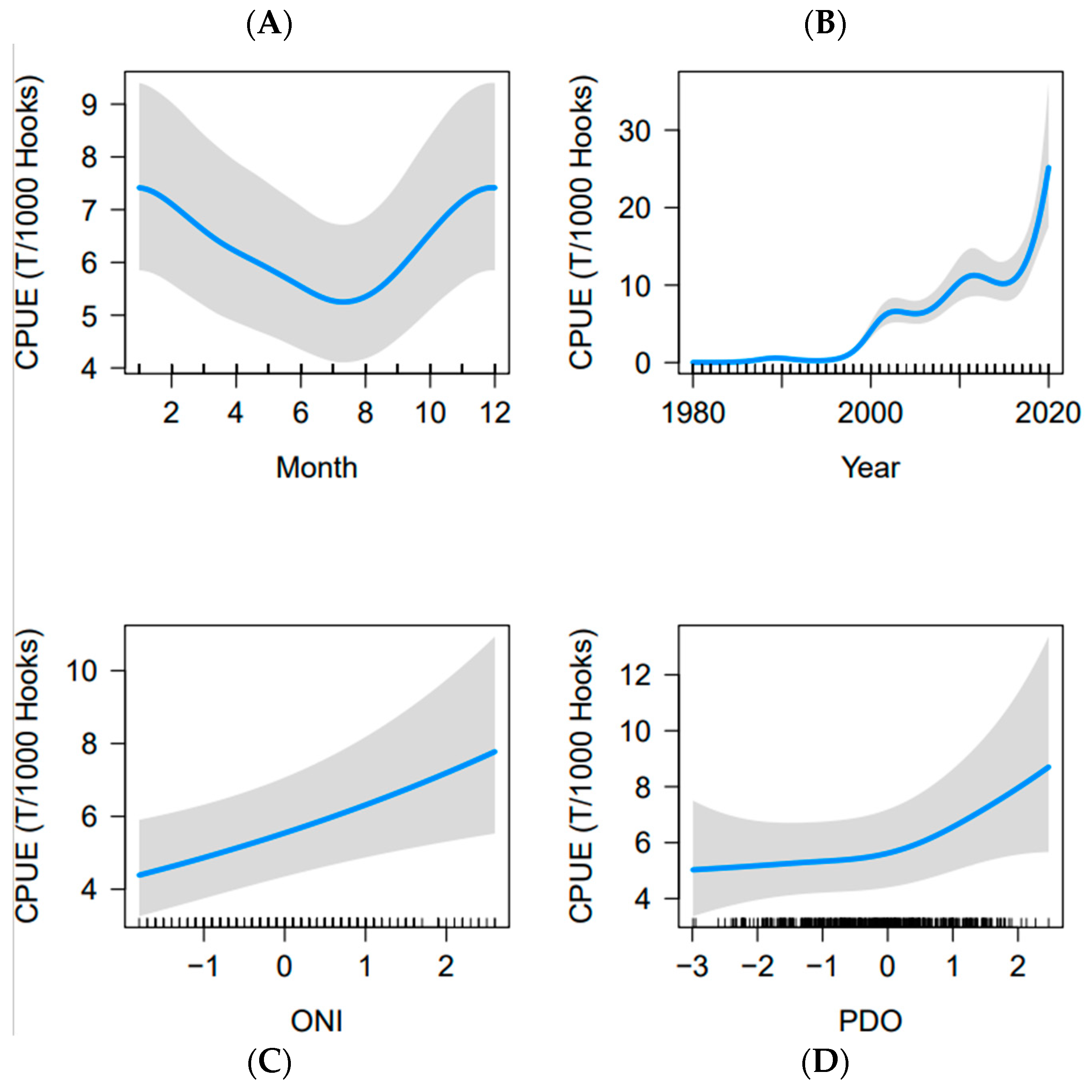
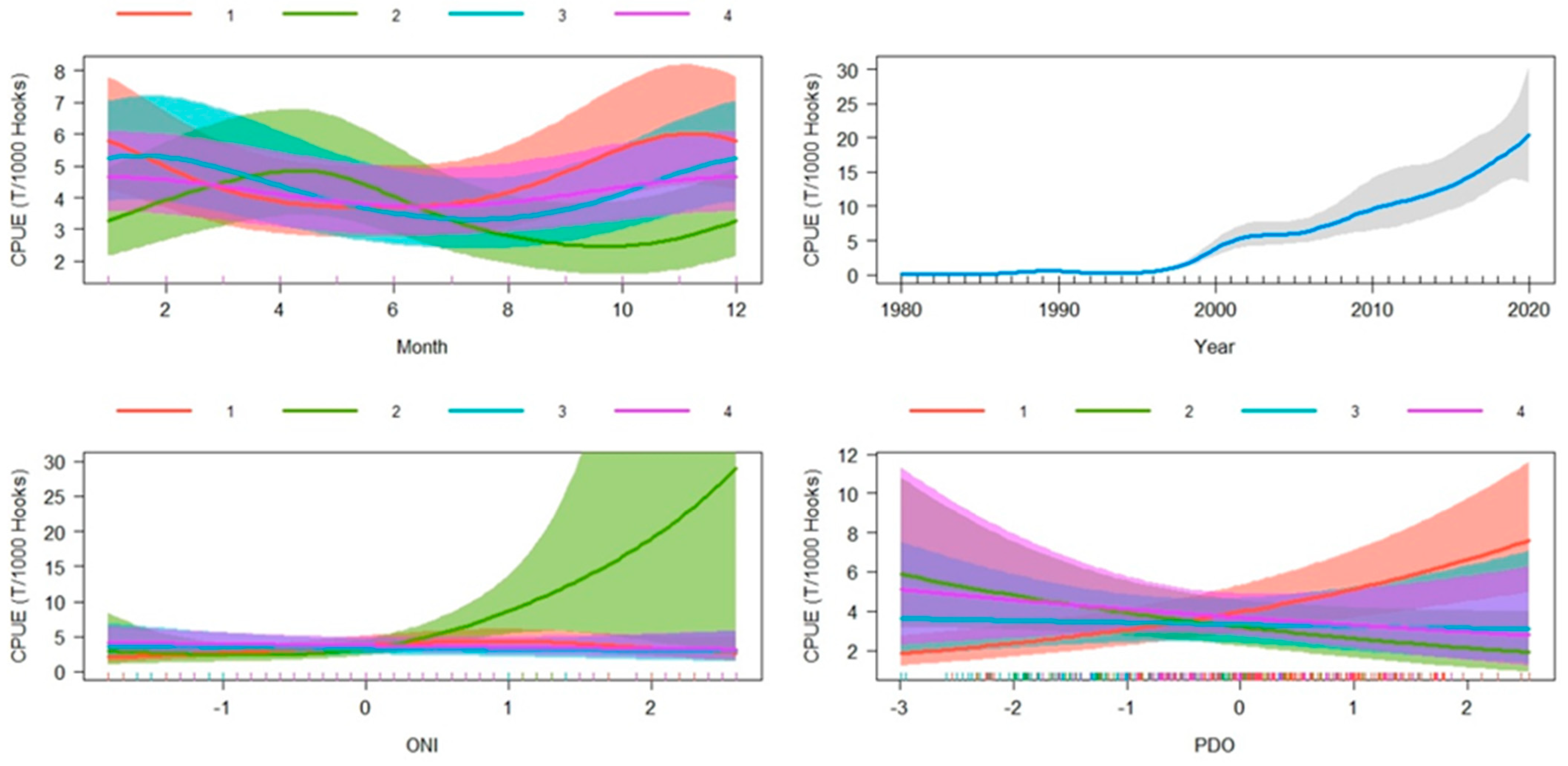
The time series of CPUE (Figure 3) for Xiphias gladius indicates an increase from the 1990s, reaching a peak in 2002, with the CPUE at May of 40 t/1000 hooks. Figure 4 shows the spatial distribution of the CPUE of X. gladius, where we can see that the largest CPUE of this species occurred in the area off the coast of Peru, mainly between 20° and 40° S and 80° and 120° W. The largest nominal CPUE was presented in the Southern Hemisphere, being the month of November the one that obtained the highest nominal CPUE with more than 20 tons per 1000 hooks. It should be noted that in the Northern Hemisphere there is a very low nominal CPUE with ranges of 0.1 to 5 tons per 1000 hooks.

3.3. GAMM

The adjusted GAMM explained 80% of the total temporal variation of the swordfish CPUE. No obvious violation of the assumptions of normality and heteroscedasticity was observed (Supplementary Figure S1). The best model included the month, the year, the ONI and the PDO, because it was the model with the lowest Akaike index obtained (

Table 1. Summary of the GAMM adjusted to the time series of the CPUE of swordfish Xiphias gladius in the Pacific. AIC = Akaike´s information criterion, ΔAIC = differences in AIC values versus minimum AIC value. s = smoothing function, p value = probability value.

Variable	AIC	ΔAIC	p Value
s(Month)	1298	392	0.156
+s(Year)	922	17	2 × 10−16
+s(ONI)	930	25	4.17 × 10−5
+s(PDO)	905	0	0.037

). In each step, the value of the concurvity was low (<0.36), suggesting no multicollinearity problem. In turn, the GAMM validation process suggested that the model has a prediction capacity of 90% (95% CI [0.85–0.93]) and an RMSE of 1.94 t/1000 hooks.

The figures of partial effect showed that the highest values of the average CPUE (~0.15 t/1000 hooks) are presented at the beginning and end of the year, presenting its lowest values (0.11 t/1000 hooks) from June to August (Figure 5A). The highest average CPUE values were observed during 2013 (~15 t/1000 hooks), with an abrupt drop after this year (~6 t/1000 hooks) (Figure 5B). Similarly, the ONI and PDO phenomena have a positive relationship with the CPUE, and mean CPUE values of ~1.5 t/1000 hooks were observed at ONI and PDO values > 1 (Figure 5C,D).

Standardized CPUE values very close to 0 were presented during the period 1980–1996. From this period, the standardized CPUE increased, presenting the highest peaks of intensity in the years 2003 and 2011, where a CPUE close to 20 t/1000 hooks was recorded. In turn, in the period from 2004 to 2005, the nominal CPUE ranged between 5 and 15 T/1000 hooks per month. It was also observed that the temporal behavior of the nominal CPUE was reflected in the final model, presenting higher nominal CPUE values at the beginning and end of each year (Figure 6).

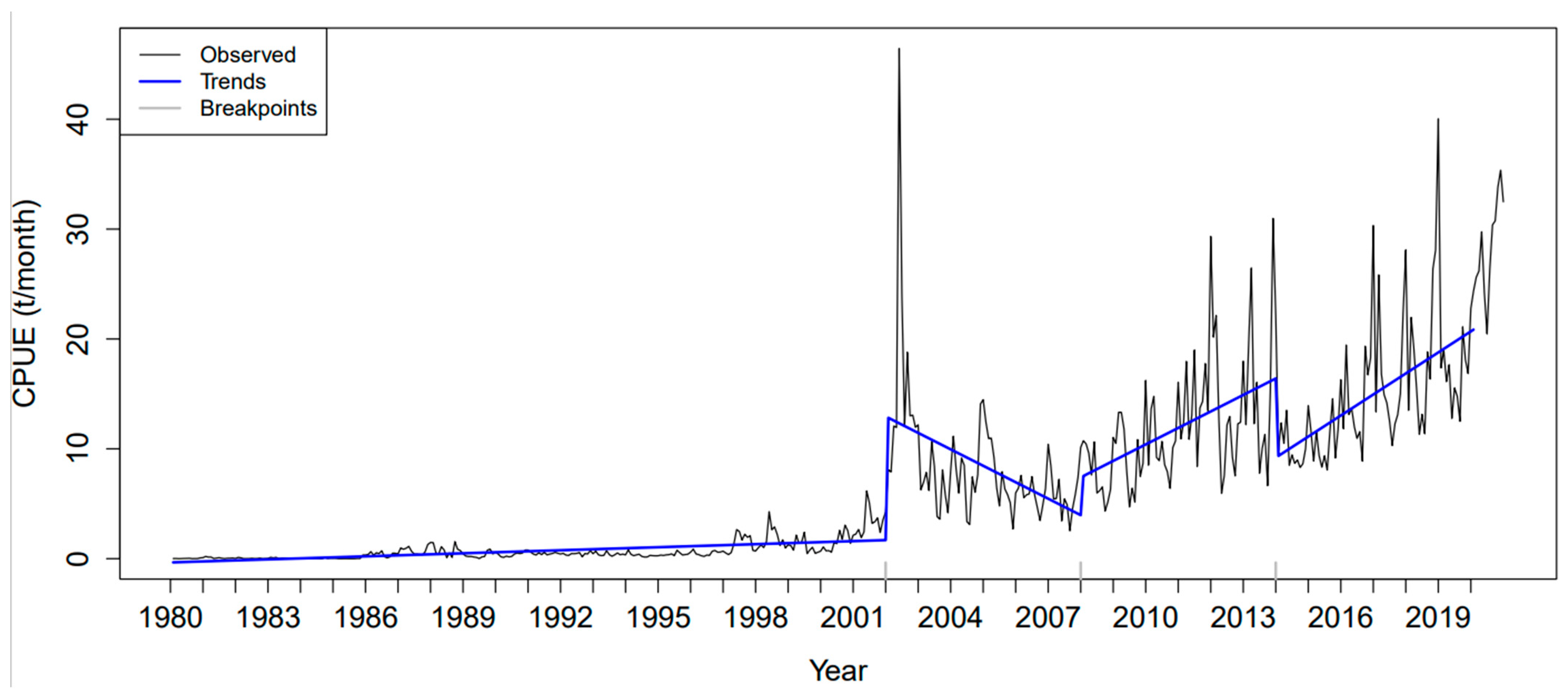
3.4. BFAST Algorithm

The BFAST algorithm found three breakpoints and four periods in the time series of the standardized CPUE, points associated with abrupt changes, thus defining four distinct periods. All of the four periods were statistically significant. In the first two periods (1980–2001 and 2001–2008) trends were observed with a monthly increase of 0.002 t/1000 hooks and a decrease −0.12 t/1000 hooks, respectively, while in the third period (2007–2013) a monthly increase of 0.03 t/1000 hooks is reported. The most important change was observed for the last period (2014–2020), with an increase in CPUE of ~0.21 t/1000 hooks per month (

Table 2. Summary of the applied linear regression models.

	Estimate	Standard Error	t Value	Pr (>|t|)
Period 1	0.00777	0.00056	13.868	2.00 × 10−16
Period 2	−0.12360	0.03020	−4.093	1.12 × 10−4
Period 3	0.12615	0.02747	4.591	1.89 × 10−5
Period 4	0.21796	0.02358	9.242	2.38 × 10−14

and Figure 7).

Once the different periods of the CPUE time series were defined with the BFAST algorithm, we fitted a new GAMM with the same structure as the model fitted to standardize the swordfish CPUE. In the new GAMM (“nested GAMM”, hereafter), we included a new factorial variable named “period”, which was included as a nested variable in the month, ONI and PDO variables, using the “by” argument of the “gamm” function. This allowed us to assess the potential nested effect of each covariate within each of the different periods of the CPUE time series.

Additionally, we computed the rate of increase r of the standardized CPUE from the nested GAMM, according to the general fishery development model proposed by FAO (https://www.fao.org/3/W3244E/w3244e0c.htm#:~:text=In%20the%20course%20of%20its,%2C%20and%20(IV)%20senescent, accessed on 10 January 2024). This model is used to assess if the landing data of a fishery follow four theoretical phases: undeveloped, developing, mature, and senescent, which depicts the actual state of the fishery. The increase rate r was calculated as r = (C_t+1 − C_t)/C_t, where C_t is the standardized CPUE at each of the months of the time series, and C_t+1 is the standardized CPUE for the next month. Values of r = 0 suggest that the fishery reached the peak of catches, which occurs during the mature phase, whereas the negative values of r suggest that the fishery is entering it senescent state, as mentioned above by FAO.

The results of the nested GAMM suggested a great variability in the effect of the covariates for each of the periods of the CPUE time series (Figure 8). For example, in period 2, CPUE values were higher during April–May when highest (>2) ONI values occurred, which was in contrast with the rest of the periods, where CPUE were higher during the last and first months of the year and at low ONI values (Figure 8).

The time series of predicted CPUE using the nested GAMM showed that the standardized CPUE increased from 1980 to 2002, remained relatively stable from 2002 to 2008, increased slightly from 2008 to 2014 (with a very noticeable seasonal variation), and increased significantly after 2014 (Figure 9).

The rate of increase suggested that the standardized CPUE has a visible high frequency variability, especially during the first two periods. After the start of the third period, the rate of increase stabilized and oscillated at approximately zero (Figure 10).

4. Discussion

4.1. Spatial–Temporal Variation in Fishing Effort

The average monthly fishing effort for the period 1980–2020 is mainly distributed southward from the equator, off the South American coast, for most of the months. This industrial longline fleet behavior of targeting swordfish could be associated with the preferred thermal distribution area of adult and sub-adult fish, likely with the abundance of prey [8]. From an oceanographic point of view, the South American coast is known for its intense upwelling events that trigger primary productivity and consequently become rich in small pelagic fishes and many squid species [27]. Surely, the swordfish longline fishers are advised by other fisheries, that in this area, the catch achievement is very high in zones where primary productions is also high. In addition, reference [13] concluded that the diet of the swordfish X. gladius caught off Baja California in northwestern Mexico is composed mainly of cephalopods (98%). X. gladius presents vertical migrations, spending in daylight many hours below the thermocline (300–1000 m), and night hours are above it. A common prey for swordfish is the giant squid Dosidicus gigas [13], an economically essential species that shares the same habitat in the Southern Hemisphere, particularly in the Southeastern Pacific Ocean, off the coasts of Chile and Peru, where the main large-scale oceanographic feature is the Humboldt Current. The high commercial importance of the area has attracted multi-national fishing vessels from Japan, Korea, Russia, China, and the local coastal countries, such as Peru, Chile, and Ecuador [28], becoming responsible for a higher proportion of total cephalopod catch in the world. It is worth noting to say that the giant squid (also known as the Humboldt squid) performs vertical migrations that are similar to those of the swordfish [29]: spending the daylight hours under the thermocline and spending night above, favoring the feeding of swordfish. Thus, the high abundances of giant squid that occur off the coast of South America could be an important factor that determinates the high swordfish CPUE. Although D. gigas is distributed from Chile in South America to California in North America [30], overlapping the range of X. gladius, the documented main fisheries grounds for the giant squid are the Southeastern Pacific waters off Chile, Peru, and Ecuador [27,30,31]. Reference [27] highlighted the ecological importance of giant squid because of its role in the food web. We believe it maintains particular importance as prey for swordfish in the Eastern Pacific Ocean.

We also analyzed the effort in the numbers of hooks deployed by the industrial swordfish longline fleet in the period of 1980–2020. Noticeable increases in fishing effort were observed during the mid-1990s, the early 2000s, and approximately during 2010. The possible explanation of the increase in effort could be related to the improvements in technology and fishery regulations such as spatial closures and the 200-mile limit decreed by some countries [32], as mentioned by [3], who cited that the number of aircraft-assisted boats had raised threefold from 1974 to 1975 in the California swordfish fishery. On the other hand, the fishery’s management may be playing an important role in the increase of efforts. If the regulations do not consider populations concept like maximum sustainable yield [3], fishers are not limited for the numbers of hooks used. Perhaps many other technologies accounted in some way to the increase in fishing efforts, but they were not considered in this study.

4.2. Spatial-Temporal Variation of the Catch per Unit of Effort CPUE

The nominal CPUE of swordfish has increased noticeably since the twenty-first century. Being different from the increasing effort mentioned in the previous section in which the increasing period of the effort started since 1975. This could be related to the need for more knowledge of species distributions and biology, like thermal preferences, feeding habits, and the differentiation in adults’ and sub-adults’ preferences. Presently, the aspects that drive migratory behavior still need to be fully understood (a similar study as the one carried out in the Atlantic Ocean by [33] is needed in the Pacific Ocean). For those reasons, the fishing areas were not well established until the twenty-first century. The CPUE in tons per 1000 hooks are higher southward from the equator. This is in concordance with the effort distribution that is being deployed in that area. The explanation is the same as mentioned in the previous section, thermal preferences and the oceanographic conditions that favor the abundance of preys in the South American coasts, mainly the presence of giant squid [27]. The thermal conditions in the fishing grounds of the Southeastern Pacific Ocean are driven by the Humboldt Current System, which exhibits changes in environmental conditions at different scales. The changes cause variations in habitat and species responses are different. For example, the El Niño occurrence in the Humboldt Current results in negative impacts of small pelagic fishes, such as sardine and anchovies, which are the preferred food source for giant squid, which is the principal food for swordfish. Environmental changes in the Humboldt Current affect the food web and, consequently, the abundance of the target fishery resource. In reference [34], it is said that: “Trophodynamics is defined as the transfer of energy from one ecosystem to another through the transfer and consumption of bioenergetic and nutritional constituents of organisms. The proposed pelagic food webs in the Southeast Pacific have shown that trophodynamics can be influenced by variability in climatic phenomena (e.g., ENSO, El Nino Southern Oscillation), as well as geographic location. The pelagic zone in the Southeast Pacific has been found to be dominated by sardine and anchovy”. The statement of reference [34] strengthened our above discussion on changes in swordfish catches.

An aspect we consider noticeable is the evolution of fishing knowledge on the species’ behavior that lets them know where to position the longlines to catch swordfish successfully because the higher effort was observed off the South American coast, which depicts the search effort of fishermen for swordfish in its feeding grounds.

4.3. CPUE Standardization (GAMM)

The results obtained applying GAMM are comparable with what reported by [19] for other billfish species, the blue marlin (Makaira nigricans) in the variables of “month” and “ONI”, likely because positive ONI phenomena present the highest CPUE. However, in the blue marlin case, extreme ONI phenomena also indicate a decrease in the CPUE. In the month’s case, the largest CPUE was presented similarly at the beginning and end of each year. These studies differ in the parameters of “year” and “PDO” since, in blue marlin, the CPUE dropped during the 1990s, while in swordfish, the opposite happened; from the 1990s, the CPUE raised. The relationship between the increase in CPUE with positive ONI phenomena agrees with what is described by [35] for the Indian Ocean, where it is mentioned that in favorable situations of the Indian Ocean Dipole, the CPUE increases since increasing the SST in the area favor the increase of primary productivity, which means that there is more food available for swordfish. Bearing in mind the extensiveness of the study area and analyzing that both the northern and southern hemispheres were included, we can establish that the results agree with [36] for the coasts of South Africa in the North Pacific but differ in the South Pacific since they propose that the highest swordfish CPUE occurred during the austral autumn–winter months (from April to July) and on the other hand, the lowest CPUE rates were present during the austral spring–summer months (October to January). Our study presented the highest CPUE rates during the months from November to February and the lowest rates during the months from June to August. These differences occur mainly because these two areas are important in terms of upwelling. In the Southeast Pacific, there is the presence of the upwellings of the Humboldt Current, which occurs mainly during the months of November to January; while in South Africa, in the Benguela Current, in winter, it also presents a high frequency of occurrence of upwellings [37].

The ONI as an index of El Niño, or strictly, the sea surface temperature (SST) anomalies are more sensitive to explain the CPUE. Reference [38] intended to explain the relationship between the abundance of swordfish (and the other two species of big pelagic fishes) and SST. They suggested that there is a threshold in SST and swordfish abundance being the 21–22 °C and a decrease in abundance at lower or higher temperatures. In the present study, we found a better index: the ONI. The catches are higher when the ONI is positive because the swordfish preys are more vulnerable due to lower turbidity [19] or because the swordfish is more vulnerable to “the baited longline hooks” as suggested by [19] who studied the blue marlin. They explained like this “probability of blue marlin encountering the baited longline hooks during positive ONI events would probably increase”.

4.4. CPUE Trends Obtained with the BFAST Algorithm

Although the factors that caused the observed CPUE trends are not fully clear, we propose some hypotheses; at the beginning of the analyzed period, this could be interpreted as changes in the technology of catches and increases in the demand for the very appreciated fish fillet of the swordfish in the last years of the twentieth century and first years of the twenty-first century. The main positive slope was observed in the second period, from 1997. Shallow pelagic longline sets that targeted swordfish started to increase in the early 1990s when fishing fleets from countries other than Japan occurred entered the swordfish fishery of the Eastern Pacific Ocean [19,39], which could help to explain the initial “boom” in the swordfish catch trends. From 2002 to 2010, the tendency decreased, perhaps resulting from the noticeable increase fishing effort exerted by Taiwanese, Chinese, and Korean vessels (Appendix A, Figure A1). This decrease was followed by a sharp increase in CPUE in 2011, which started another decrease. However, the linear regression slope in that period was not significant, suggesting a steady period. That means a stable tendency. Reference [19] suggested that a decrease in the fishing effort of the longline fleet occurred during 2010 when the swordfish CPUE increased from approximately 6 to 100 t/month. According to NOAA’s SMART stock website (https://apps-st.fisheries.noaa.gov/stocksmart?stockname=Swordfish%20-%20Eastern%20Pacific&stockid=11643, accessed on 9 November 2022), the swordfish stock of the Eastern Pacific Ocean was not overexploited during 2010. Then, a plausible explanation for the increase in swordfish CPUE during 2010 is that it is the result that a similar amount of swordfish biomass was available when low fishing effort occurred, thus resulting in higher CPUE. We also acknowledge that the differences in targeting species of the fleet and perhaps the enormous extension of our study area could also influence the CPUE trends we observed. However, high year-to-year variability in swordfish CPUE has been observed for more restricted localities, such as the southern California waters (the northern frontier of their range in the Eastern Pacific) [3], so we consider that the results of analyzing data from a large area could be like those data of restricted areas.

We also consider it important to highlight a very important variable that is not being considered in our analysis: swordfish size. Changes in fishing practices could be resulting in a decrease in mean swordfish size (for example, an increase in the longline sets near floating objects, important zones of congregation for immature billfish and tuna), which in turn would affect the CPUE biomass. Unfortunately, to the best of the authors’ knowledge, there is no IATTC data (at least not in their public repository) of the size frequencies of swordfish caught by the longline fleet in the EPO. We encourage future research to assess the potential changes in mean swordfish size, because such changes could jeopardize the future of the fishery if too many immature swordfish are caught by the fleet.

We also noticed a great variability in the effects of the covariates on the swordfish CPUE within each of the time periods. To investigate the potential causes of such variability is outside the scope of our research, and it opens a very promising research field in future study.

We could not observe any of the theoretical fishery development phases suggested by FAO. A possible cause for this is that, as FAO mentioned, “the natural variability of individual fisheries is probably too high, and the potential causes of variation in landings are too numerous to any allow any safe interpretation and extrapolation of observed trends”. This was apparently the case of our contribution because we observed a noticeable high frequency variability in the swordfish CPUE time series. We believe that this is a very interesting result, and the potential causes of such high variability should be further investigated.

4.5. Possible Fishery Implications

The present study, targeted to obtain maps illustrating seasonal changes in the spatial distribution and to determine which environmental variables influenced swordfish occurrence in the EPO. Knowledge on suitable conditions for the species may be used to assess possible habitat variations during extreme oceanographic events, such as El Niño. Although both variables that were used as proxy for variations in the marine climate (ONI and PDO) on the interannual and decadal scale resulted to be significant, they were responsible for a low change in AIC, when compared to the year. This suggests that although the effect of the marine climate in swordfish CPUE is noticeable, there are other factors that are more important, factors that are perhaps the result of change in fleet; we suggest that the potential combined effect of variations in the marine environment and changes in fleet dynamics is a very important subject, and it should be further investigated. The monthly CPUE maps could also be used to make some inferences on swordfish migration patterns in the region. Generally, the information provided by this study could contribute to the better management of swordfish. However, we recommend that fisheries scientists and fisheries managers take this finding with caution to reach a sustainable exploitation of the swordfish fishery resource, because further analysis, such as species distribution models, might provide a more comprehensive view of the environmental effects on the spatial and temporal variations of the incidental catches of swordfish. Consequently, species distribution models may reveal patterns that help to understand the behavior of important fishery resources and can provide policy makers with some of the scientific information required to develop management plans, which are crucial for the rational and sustainable harvesting of natural resources.

5. Conclusions

The oceanographic factors, such as El Niño events and the Pacific Decadal Oscillation, positively influence swordfish CPUE, perhaps due to changes in prey availability and in the increase of vulnerability to baited fishing hooks that result from changes in water turbidity. It is possible to make catch predictions based only on environmental data for the model. According to the BFAST model, the current trend of swordfish fishing is downward. It is recommended to take this finding with caution to obtain a sustainable exploitation of the swordfish fishery resource.

References

1. Lecointre, G.; Le Guyader, G. Classification Phylogénétique du Vivant; Editions Belin: Paris, France, 2006; pp. 1–544. [Google Scholar]
2. Nakamura, I. Billfishes of the World. An Annotated and Illustrated Catalogue of Marlins, Sailfishes, Spearfishes and Swordfishes Known to Date; FAO: Rome, Italy, 1985; pp. 1–65. [Google Scholar]
3. Bedford, D.; Hagerman, F. The billfish fishery resources of the California Current. CALCOFI Rep. 1983, 24, 70–78. [Google Scholar]
4. Takahashi, M.; Okamura, H.; Yokawa, K.; Okazaki, M. Swimming behavior and migration of a swordfish recorded by an archival tag. Mar. Fresh Res. 2003, 54, 527–534. [Google Scholar] [CrossRef]
5. Lobell, M.J. The Fisheries of Chile, Present Status, and Future Possibilities (United States Fisheries Mission to Chile); U.S. Department Interior, Fish Wildlife Service: Washington, DC, USA, 1947; pp. 14–20.
6. Fitch, J.E. Swordfish; California Department of Fish and Game: Sacramento, CA, USA, 1960; pp. 1–79.
7. Palko, B.J.; Bearsdley, G.L.; Richards, W.J. Synopsis of the Biology of the Swordfish, Xiphias gladius Linnaeus; FAO: Rome, Italy, 1981; pp. 1–21. [Google Scholar]
8. Mejuto-García, J. Aspectos Biológicos y Pesqueros del Pez Espada (Xiphias gladius Linnaeus, 1758) del Océano Atlántico, con Especial Referencia a las Áreas de Actividad de la Flota Española. Ph.D. Thesis, Universidad de Santiago de Compostela, Galicia, Spain, 2007. [Google Scholar]
9. Abecassis, M.; Dewar, H.; Hawn, D.; Polovina, J. Modeling swordfish daytime vertical habitat in the North Pacific Ocean from pop-up archival tags. Mar. Ecol. Prog. Ser. 2012, 452, 219–236. [Google Scholar] [CrossRef]
10. Moreira, F. Food of the swordfish, Xiphias gladius Linnaeus, 1758, off the Portuguese Coast. J. Fish. Biol. 1990, 36, 623–624. [Google Scholar] [CrossRef]
11. Hernández-García, V. The diet of the swordfish Xiphias gladius Linnaeus, 1758, in the central east Atlantic, with emphasis on the role of cephalopods. Fish. Bull. 1995, 93, 403–411. [Google Scholar]
12. Markaida, U.; Sosa-Nishizaki, O. Food and feeding habits of Swordfish, Xiphias gladius L., off Western Baja California. In: Biology and fisheries of swordfish Xiphias gladius. NOAA Tech. Rep. NMFS 1998, 142, 1–276. [Google Scholar]
13. Trujillo-Olvera, A.; Ortega-Garcia, S.; Tripp-Valdez, A.; Escobar-Sanchez, O.; Acosta-Pachón, T.A. Feeding habits of the swordfish (Xiphias gladius Linnaeus, 1758) in the subtropical northeast Pacific. Hydrobiologia 2018, 822, 173–188. [Google Scholar] [CrossRef]
14. Abascal, F.J.; Mejuto, J.; Quintans, M.; Ramos-Cartelle, A. Horizontal and vertical movements of swordfish in the Southeast Pacific. ICES J. Mar. Sci. 2010, 67, 466–474. [Google Scholar] [CrossRef]
15. Sosa-Nishizaki, O. Revisión histórica del manejo de los picudos en el Pacífico mexicano. Cienc. Mar. 1998, 24, 95–111. [Google Scholar] [CrossRef]
16. Fleischer, L.A.; Traulsen, A.K.; Ulloa-Ramírez, P.A. Mexican progress report on the marlin and swordfish fishery. In Proceedings of the Working Document Submitted to the ISC Billfish Working Group Workshop, Honolulu, HI, USA, 3–10 February 2009. [Google Scholar]
17. Folsom, B.W.; Weidner, D.M.; Wildman, M.R. An Analysis of Swordfish Fisheries, Market Trends, and Trade Patterns Past-Present-Future; U.S. Department of Commerce: Silver Spring, MD, USA, 1997. Available online: https://repository.library.noaa.gov/view/noaa/33517 (accessed on 15 March 2024).
18. Squire, J.L.; Muhlia-Melo, A.F. A review of striped marlin (Tetrapturus audax), swordfish (Xiphias gladius), and sailfish (Istiophorus platypterus) fisheries and resource management by Mexico and the United States in the northeast Pacific Ocean. NOAA NMFS SWFSC Adm. Rep. 1993, lj-93-96, 1–44. [Google Scholar]
19. Marín-Enríquez, E.; Abitia-Cárdenas, L.A.; Moreno-Sánchez, X.G.; Ramírez-Pérez, J.S. Historical analysis of blue marlin (Makaira nigricans Lacepède, 1802) catches by the pelagic longline fleet in the eastern Pacific Ocean. Mar. Freshw. Res. 2020, 71, 532–541. [Google Scholar] [CrossRef]
20. Wyrtki, K. An estimate of equatorial upwelling in the Pacific. Am. Meteorol. Soc. 1981, 11, 1205–1214. [Google Scholar] [CrossRef]
21. Zhang, Y.; Wallace, J.M.; Battisti, D.S. ENSO-like interdecadal variability. J. Climate 1997, 10, 1004–1020. [Google Scholar] [CrossRef]
22. Mantua, N.J.; Hare, S.R. The Pacific decadal oscillation. J. Oceanogr. 2002, 58, 35–44. [Google Scholar] [CrossRef]
23. Newman, M.; Alexander, M.A.; Ault, T.R.; Cobb, K.M.; Deser, C.; Di Lorenzo, E.; Mantua, N.J.; Miller, A.J.; Minobe, S.; Nakamura, H.; et al. The Pacific Decadal Oscillation, Revisited. J. Climate 2016, 29, 4399–4427. [Google Scholar] [CrossRef]
24. Zuur, A.F.; Ieno, E.N.; Walker, N.J.; Saveliev, A.A.; Smith, G.M. Mixed Effects Models and Extensions in Ecology with R.’; Springer: New York, NY, USA, 2009; pp. 1–458. [Google Scholar]
25. Burnham, K.P.; Anderson, D.R. Model Selection and Multimodel Inference: A Practical Information-Theoretic Approach, 2nd ed.; Springer: New York, NY, USA, 2002; pp. 1–488. [Google Scholar]
26. Verbesselt, J.; Hyndman, R.; Zeileis, A.; Culvenor, D. Phenological Change Detection While Accounting for Abrupt and Gradual Trends in Satellite Image Time Series. Remote Sens. Environ. 2010, 114, 2970–2980. [Google Scholar] [CrossRef]
27. Feng, Z.; Yu, W.; Chen, X. Concurrent habitat fluctuations of two economically important marine species in the Southeast Pacific Ocean off Chile in relation to ENSO perturbations. Fish. Oceanogr. 2022, 31, 123–134. [Google Scholar] [CrossRef]
28. Morales-Bojorquez, E.; Pacheco-Bedoya, J.L. Jumbo squid Dosidicus gigas: A new fishery in Ecuador. Rev. Fish. Sci. Aquac. 2016, 24, 98–110. [Google Scholar] [CrossRef]
29. Gilly, W.F.; Markaida, U.; Baxter, C.H.; Block, B.A.; Boustany, A.; Zeidberg, L.; Reisenbichler, K.; Robinson, B.; Bazzino, G.; Salinas, C. Vertical and horizontal migrations by jumbo squid, Dosidicus gigas, revealed by electronic tagging. Mar. Ecol. Prog. Ser. 2006, 324, 1–17. [Google Scholar] [CrossRef]
30. Markaida, U.; Quiñonez-Velázquez, C.; Sosa-Nishizaki, O. Age, growth, and maturation of jumbo squid Dosidicus gigas (Cephalopoda: Ommastrephidae) from the Gulf of California, Mexico. Fish. Res. 2004, 66, 31–47. [Google Scholar] [CrossRef]
31. Estrella-Arellano, C.; Swartzman, G. The Peruvian artisanal fishery: Changes in patterns and distribution over time. Fish. Res. 2010, 101, 133–145. [Google Scholar] [CrossRef]
32. Bayliff, W.H. The Fisheries for Tunas in the Eastern Pacific Ocean. In Advances in Tuna Aquaculture. From Hatchery to Market; Benetti, D.D., Partridge, G.J., Buentello, A., Eds.; Academic Press: Oxford, UK, 2016; pp. 21–41. [Google Scholar]
33. Neilson, J.D.; Loefer, J.; Prince, E.D.; Royer, F.; Calmettes, B.; Gaspar, P.; Lopez, R.; Andrushchenko, I. Seasonal Distributions and Migrations of Northwest Atlantic Swordfish: Inferences from Integration of Pop-Up Satellite Archival Tagging Studies. PLoS ONE 2014, 9, e112736. [Google Scholar] [CrossRef]
34. Quispe-Machaca, M.; Guzmán-Rivas, F.A.; Ibañez, C.M.; Urzúa, A. Trophodynamics of the jumbo squid Dosidicus gigas during winter in the Southeast Pacific Ocean off the coast of Chile: Diet analyses and fatty acid profile. Fish. Res. 2022, 245, 106154. [Google Scholar] [CrossRef]
35. Lan, K.-W.; Lee, M.-A.; Wang, S.-P.; Chen, Z.-Y. Environmental variations on swordfish (Xiphias gladius) catch rates in the Indian Ocean. Fish. Res. 2015, 166, 67–79. [Google Scholar] [CrossRef]
36. Parker, D.; Winker, H.; West, W.; Kerwath, S.E. Standardization of the catch per unit effort for swordfish (Xiphias gladius) for the South African longline fishery. Sci. Pap. ICCAT 2017, 74, 1295–1305. [Google Scholar]
37. Shumann, E.H.; Perris, L.A.; Hunter, I.T. Upwelling along the South Coast of the Cape Province, South Africa. S. Afr. J. Sci. 1982, 78, 238–242. [Google Scholar]
38. Santana-Hernández, H.; Macías-Zamora, R.; Vidaurri-Sotelo, A. Relación entre la abundancia de peces de pico y la temperatura del agua en el Pacífico mexicano. Cienc. Pesq. 1996, 13, 62–65. [Google Scholar]
39. Hinton, M.G.; Bayliff, W.H.; Suter, J.M. Assessment of swordfish in the eastern Pacific Ocean. In Proceedings of the ‘5th Meeting. Document SAR-5-05-SWO’, La Jolla, CA, USA, 11–13 May 2004; Inter-American Tropical Tuna Commission, Working Group on Stock Assessment: La Jolla, CA, USA. [Google Scholar]
Figure 1. Spatial distribution of fishing effort of Xiphias gladius swordfish, from January 1980 to December 2020. Color palette depicts fishing effort in millions of hooks.
Jmse 12 00496 g001
Figure 2. Hovmöller diagram of the temporal variation of the effort for Xiphias gladius reported by the industrial longline fleet in the Eastern Pacific Ocean.
Jmse 12 00496 g002
Figure 3. Time series of catch per unit effort (CPUE) for the swordfish fishery Xiphias gladius in the Pacific.
Jmse 12 00496 g003
Figure 4. Spatial distribution of the nominal catch per unit effort (CPUE; tons per 1000 hooks) of swordfish Xiphias gladius, from January 1980 to December 2020.
Jmse 12 00496 g004
Figure 5. Partial effect graphs of the explanatory variables of the GAMM adjusted to the time series of the CPUE of swordfish Xiphias gladius.
Jmse 12 00496 g005
Figure 6. Time series of the swordfish CPUE Xiphias gladius from 1980 to 2020. The blue line shows the fit of the GAMM using year, month, ONI, and PDO data.
Jmse 12 00496 g006
Figure 7. CPUE time series trends of swordfish Xiphias gladius obtained from the BFAST algorithm.
Jmse 12 00496 g007
Figure 8. Partial effect plots of the nested GAMM. The curves in each of the covariates (not including Year) represent the effect of the covariate on the swordfish CPUE, for each of the periods obtained from the BFAST algorithm.
Jmse 12 00496 g008
Figure 9. Time series of the standardized swordfish CPUE for each of the periods obtained from the BFAST algorithm, computed using the nested GAMM.
Jmse 12 00496 g009
Figure 10. Increase rate of the swordfish standardized CPUE computed with the nested GAMM. The vertical dashed lines depict each of the periods obtained from the BFAST algorithm, and the continuous horizontal line shows the theoretical value of r = 0.
Jmse 12 00496 g010