Flow and Cavity Measurements in a Super-Cavitating Propeller

Abstract

The design of super-cavitating propellers takes advantage of the development of air cavities on the blades’ surface to reduce drag and, ultimately, increase efficiency. The mechanism of flow modification induced by the development of a cavity on the propeller blades was investigated experimentally via phase-locked laser Doppler velocimetry measurements. A large cavity extending beyond the blades’ trailing edge and enclosing the back of the blades was identified at high loading conditions. A robust methodology to quantitatively analyze the size of the cavity is presented. The analysis of the flow fields showed that, under fully developed cavitation conditions, the acceleration of the axial and tangential flow in the inter-blade region was observed, accompanied by a reduction in tip-vortex development.

1. Introduction

One of the most-critical physical phenomena that may affect bodies moving in water is cavitation. Cavitation occurs when the fluid static pressure drops below the vapor pressure. In this situation, vapor cavities form within the fluid. Their sudden collapse leads to a range of detrimental effects, such as a loss in performance, structural vibrations, increased radiated noise emission, and surface erosion [1]. In fact, hydro-machines, in general, are designed to avoid cavitation inception within their operating range. An exception to this scenario is found in a particular category of fast-moving bodies comprising projectiles, torpedoes, and high-speed propellers. In these applications, the moving body is designed to exploit the occurrence of cavitation. At specific flow velocities, a large and persistent cavity forms around the body, extending beyond its size, and works as a drag-reducing mechanism. For propellers designed according to this principle, called super-cavitating propellers, another advantage is represented by the collapsing of bubble cavities, which is most likely to occur far from the blades’ surface, thus avoiding the erosion process [2]. For these reasons, super-cavitating propellers are considered to be among the most-efficient propulsors for high-speed vessels.

Most of the literature on super-cavitating bodies focuses on projectiles of different shapes (see [3,4,5,6]), whereas the characterization of the flow around super-cavitating propellers remains relatively unexplored. Furthermore, most of the work consists of numerical simulations [7,8]. In [9], for instance, the Boundary Element Method was used to predict the cavitation patterns on a super-cavitating propeller in steady and unsteady flow.

The experimental measurement of cavitating flows is characterized by many difficulties. The use of optical methodologies is hindered by the intrinsic presence of reflections caused by the incident light on the bubbles and cavity surfaces. The study of the flow around a propeller is made more complicated by the inherent low accessibility to the inter-blade space and the propeller rotation itself. Investigations on cavitating flow around a propeller can be found in [10,11] for uniform and non-uniform flow, respectively. In the latter work, a methodology for cavity surface measurement based on image processing was presented. A review of different methodologies for cavitation pattern measurement can be found in [12]. In [13], high-speed imaging was used to investigate the tip cavitation, whereas in [14], the authors focused on the radiated noise induced by cavitation in tunnel and real-world tests. Cavitation in non-uniform flow conditions was also addressed numerically in [15,16]. Laser Doppler velocimetry (LDV) was used to investigate cavitating flows developing on hydrofoils in [17,18], with the latter focusing on cavitation-induced vibrations. Furthermore, LDV was employed to analyze tip-vortex cavitation stemming from elliptic foils in [19,20,21], in some cases in combination with high-speed imaging.

In this work, we analyze the flow around a super-cavitating propeller at three loading conditions by means of LDV. The role of the developed cavitation patterns on the propeller hydrodynamics is explored by considering three operating conditions: non-cavitating flow, mild cavitating flow, and fully cavitating flow. The latter is identified as the super-cavitating condition. Despite its reliance on laser light, the working principle of LDV, that is the Doppler shift of the light scattered by a tracer particle crossing the measurement volume, makes it a very robust technique against cavity reflections. We demonstrate how this aspect stands as a distinctive advantage with respect to other techniques, such as Particle Image Velocimetry (PIV), and allows high accessibility to the inter-blade flow. Furthermore, the presented approach allows quantitative cavity volume measurement, which is crucial for the validation of simulation codes. The aim of this work is, therefore, twofold. We first determine the ability of an LDV-based approach to analyze cavitating flows. Subsequently, this approach is applied to a super-cavitating propeller in order to shed light on the modification of the inter-blade flow induced by the cavity development.

2. Materials and Methods

2.1. Experimental Setup

The experimental campaign was conducted at the Italian Navy Cavitation Tunnel Facility (CEIMM), located at CNR-INM. The test section was square, 0.6 m in width with rounded edges and a length of 2.6 m. Upstream of the test section, the convergent section had a contraction ratio of 6:1. The free-stream velocity range was 2–12 m/s, with an estimated maximum free-stream turbulence intensity of 2% inside the test section. The pressure inside the tunnel can be controlled in the range of 1750 mbar to 150 mbar to achieve the desired cavitation number, as described later. Perspex windows allowed optical access from all four sides of the test chamber.

The propeller under consideration was composed of three blades, with a diameter $D=220$ mm, and was mounted on a dynamometer with an embedded encoder (0.1° resolution). Flow measurements were obtained via a two-component back-scatter LDV system, consisting of a 2-component optic probe and a 40 MHz Bragg cell, necessary to remove the directional ambiguity of the velocity. The LDV optics were equipped with a 500 mm focal lens, resulting in a measurement volume with dimensions of 0.3 × 0.3 × 2.5 mm.

The data management and acquisition were carried out via TSI’s Flowsizer V6 software. The visualization of the cavitation patterns was simultaneously achieved by two high-speed cameras (SA1.1 CMOS Photron FastCam, 12-bit dynamic range, 1024 × 1024 px image resolution), positioned approximately 100° apart to view the pressure and suction sides of the propeller. The LDV system’s head was mounted on a traversing system actuated by electric motors, allowing the movement along the three directions of the test section’s reference frame with an accuracy of 0.05 mm.

Considering the inherent radial symmetry of the propeller inflow and the steady conditions, it was possible to attain the full three-component velocity field in the propeller reference system. For each location along the X axis (i.e., the downstream direction), acquisitions were carried out on two grid lines: along the Y and Z directions separately, as seen in Figure 1. Since the LDV probe volume captures simultaneously two perpendicular velocity components, data collected along the Y direction provided the axial and radial velocity components, while the axial and tangential components were obtained along the Z direction. In other words, and because of the rotation of the propeller, all measurement points on a circular path in the propeller frame of reference were obtained without changing the position of the LDV head. A sketch of the experimental setup is provided in Figure 2. The grid lines along the Y and Z coordinates had 22 sample points each. The measurement points were unevenly spaced, with a higher density around the blade tips. The grid points were arranged according to a Cartesian system with the origin at the center of the propeller disc. The X axis was coincident with the shaft axis, fore–aft-oriented.

The acquisitions were performed at six positions along the X direction, as reported in

Table 1. List of acquisition planes along the X coordinate; absolute value and normalized to propeller radius R = D/2.

Plane	X (mm)	$\mathit{X}/\mathit{R}$
1	0	0
2	28	0.26
3	56	0.50
4	73	0.66
5	87	0.80
6	103	0.94

. According to this setup, the total number of grid points was 264 for each test case. Schematics of the resulting points’ grid after the phase-locking arrangement are provided in Figure 1.

A phase-locking methodology was employed to categorize the collected data, as described in [22]. Whenever a Doppler signal was detected in any of the two LDV channels, a velocity sample was stored. Each sample was tagged with the corresponding blade angular position provided by the shaft encoder. With this information, the data were sorted in the post-processing step according to angular slots of equal size to obtain velocity statistical quantities such as the mean and root mean square (RMS). The choice of the slot size is pivotal in phase-locking schemes, as a trade-off between data resolution and data convergence must be considered [23]. In the current work, a slot of 2° was set with an overlap of 50% between slots. No window function was used to weigh the samples.

For each measurement point in the grid, the acquisition time window was set to 45 s, with the acquisition rate ranging between 4000 and 10,000 Hz. The duration time was set according to a trade-off between the data resolution, according to the phase-locking scheme described above, and the overall time consumption. With this aim and to improve the data rate of the Doppler signal processor, the working fluid was seeded with 1 $\mathsf{\mu }$m titanium dioxide tracer particles.

The test matrix is summarized in

Table 2. Test cases.

Advance Ratio J		Cavitation Number $\mathit{\sigma }$
0.7	15	7.3	1.5
1.0	15	7.2	1.5
1.3	15	6.8	1.5

. We point out that the conditions tested correspond to a propeller running in a uniform wake field. Nevertheless, the methodology presented can also be applied to non-uniform inflow conditions, such as those usually encountered when the propeller is operating behind a ship hull. The advance ratio is defined as $J=U_0/nD$, where $U_0$ is the free-stream flow velocity and n is the propeller rotation rate, expressed as revolutions per second. The advance ratio is associated with blade loading, with lower values corresponding to higher loading. Three cavitation numbers were selected and investigated for each loading condition, according to the type of cavitation patterns observed via the high-speed visualizations, as explained in Section 3.1. Pressure P inside the test section was adjusted to obtain the desired cavitation conditions. The corresponding cavitation number based on the propeller revolution rate was $\sigma =2(P-P_v)/\rho n^2{D}^2$, where $P_v$ and $\rho$ are the water vapor pressure and density at the testing temperature, respectively. The cavitation number is a non-dimensional quantity used to qualify the cavitation state of a flow, from no cavitation to cavitation inception to developed cavitation. In order to highlight the modification of the surrounding flow as cavitation develops, three cavitating conditions were analyzed: no cavitation (high σ); leading edge/mid-chord cavitation (mid-σ); fully developed cavitation (low σ).

2.2. Uncertainty Analysis

The main sources of error in the measurement chain of the current setup were positioning errors and data-processing errors. The positioning errors were due to: (1) the accuracy of the motorized traversing system transporting the LDV head, which was 0.05 mm; (2) the alignment of the measurement probe on the origin of the coordinate system, whose uncertainty was 0.5 mm. On the other hand, the data-processing errors stemmed from the slotting technique used to sort the recorded data, as described in the previous section. As pointed out in [22], the averaging operation within each slot worked as a low-pass filter of the gradients along the tangential direction, and its effect was found to be negligible for slotting sizes up to 2°.

The uncertainty of the statistical quantities was estimated based on the Student’s t-distribution. Defined as $t_{0.975\left(N\right)}$, the Student’s t value corresponding to a confidence level of 97.5% and sample size N, the standard error of the mean of the general velocity component v was calculated as $v_{err}=\pm t_{0.975\left(N\right)}RMS\left(v\right)/\sqrt{N-1}$. According to this, the measurement uncertainty on the velocity components was between 0.06% and 2.3%.

3. Results

3.1. Identification of Cavitation Regimes

The identification of the cavitation pattern is pivotal both as a preliminary stage to set up the test matrix for the campaign and as a support tool to analyze the flow field. At a fixed free-stream speed and propeller rotation rate, the pressure inside the test chamber was gradually reduced until cavitation was visually detected. As $\sigma$ decreases, cavitation develops in progressive stages. As expected, the first stage encountered is blade tip cavitation, shown in Figure 3 at an advance coefficient $J=1.0$ and $\sigma =7.2$, which also highlights the tip-vortex evolution within the propeller wake. The next stage, observed at $J=0.7$, $\sigma =7.3$, features a pattern of leading-edge cavitation associated with a cloud-like pattern along the tip-vortex wake path, thought to be related to the instability of the tip-vortex, shown in Figure 4. At $J=1.0$, $\sigma =1.5$, the cavity extends from the leading edge up to the mid-chord section of the blade, as shown in Figure 5. The last stage was observed for $J=0.7$, $\sigma =1.5$, and is shown in Figure 6. A large cavity develops on the suction surface of the blades and extends beyond the trailing edge. The cavity closure takes place in the fluid away from the trailing edge and appears as a foamy bubble cloud. The low-pressure side of the blade appears to be immersed in the cavity and in a dry state. Under these conditions, the blade back is fully enclosed in the cavity, realizing the super-cavitating condition. The visualization results are summarized in

Table 3. Identified cavitation patterns.

J	$\mathit{\sigma }$ = 15	$\mathit{\sigma }$ = 6.8–7.3	$\mathit{\sigma }$ = 1.5
0.7	no cavitation	leading edge + tip	full (super-cavity)
1.0	no cavitation	tip	mid-chord + tip
1.3	no cavitation	no cavitation	mid-chord + tip

.

3.2. Cavity Size Estimate

A challenging task when dealing with cavitating flows is to reliably assess the cavity size. This not only relates to the extension of the vapor cavity, but also to its stability over time. In this section, we demonstrate how the chosen methodology allows for a reliable estimate of the three-dimensional extension of the cavitating flow regions. We recall that, when the LDV measurement volume is inside a solid body, such as the propeller or a vapor-filled region, no data samples are collected. The absence of the Doppler signal is due to the lack of seeding particles in the vapor-filled regions, as well as to the misalignment of the LDV laser beams when crossing the water–vapor interface due to refraction.

By comparing the LDV results between the non-cavitation and cavitation cases, it is possible to assess the cavity extension. This principle is schematized in Figure 7, where the number S, defined as the average number of samples per slot, is shown versus the angular position $\theta$ for the three tested $\sigma$ values. These data were obtained at the radial position $r=0.7R$ and downstream location $X/R=0.50$ (corresponding to plane 3) and serve as an example of the methodology approach applicable at any measurement point.

Given the three-blade geometry of the propeller, the samples’ trend features a periodic pattern along the entire angle range. An interval, approximately between $\theta ={75}^{\circ }$ and $\theta ={130}^{\circ }$, is characterized by a drop of S down to a null value, with the extension of the drop depending on $\sigma$. At the lower end of the interval, as depicted in the left inset, the steep decrease from the average level of samples (i.e., $S=1$) to null occurs regardless of the cavitation number, indicating that the drop is caused by the measurement volume intersecting the propeller blade, specifically the blade pressure side. Since the number of collected samples is directly related to the flow speed within the measurement volume, the steep drop, covering approximately a two-degree span, is associated with the boundary layer over the blade surface. At the higher end of the interval, the behavior varies depending on $\sigma$, as better highlighted in the right inset. For non-cavitating conditions, the rise in the number of acquired samples indicates that the acquisition volume is leaving the back of the blade. On the other hand, the recovery from $S=0$ in the case of $\sigma =1.5$ occurs 19° later than the higher $\sigma$ cases. This indicates that the measurement volume is crossing the cavity along an interval spanning 19°, based on the data resolution. Furthermore, since no valid sample was acquired for these points over the measurement time, it follows that the cavity is quite stable, and a reliable assessment of its size may be directly obtained.

Since the probe volume has a finite size, we point out that it could intersect partially the propeller/cavity, resulting in a decrease in the number of recorded samples. The accuracy on the identification of the cavity border is then strictly related to the size of the measurement probe volume and to the chosen slot size. In Figure 8, similar plots are shown for all six planes along the X coordinate.

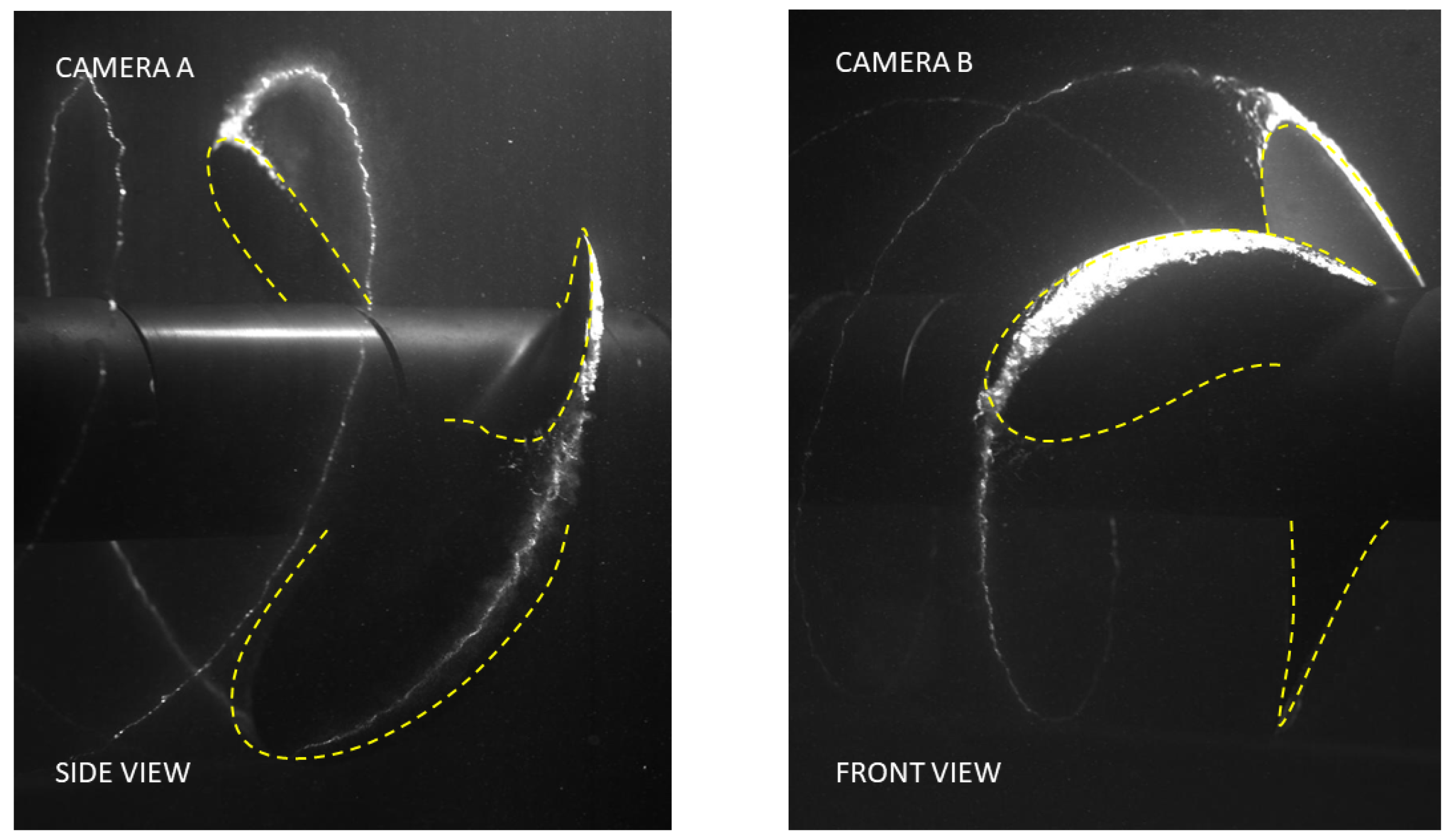
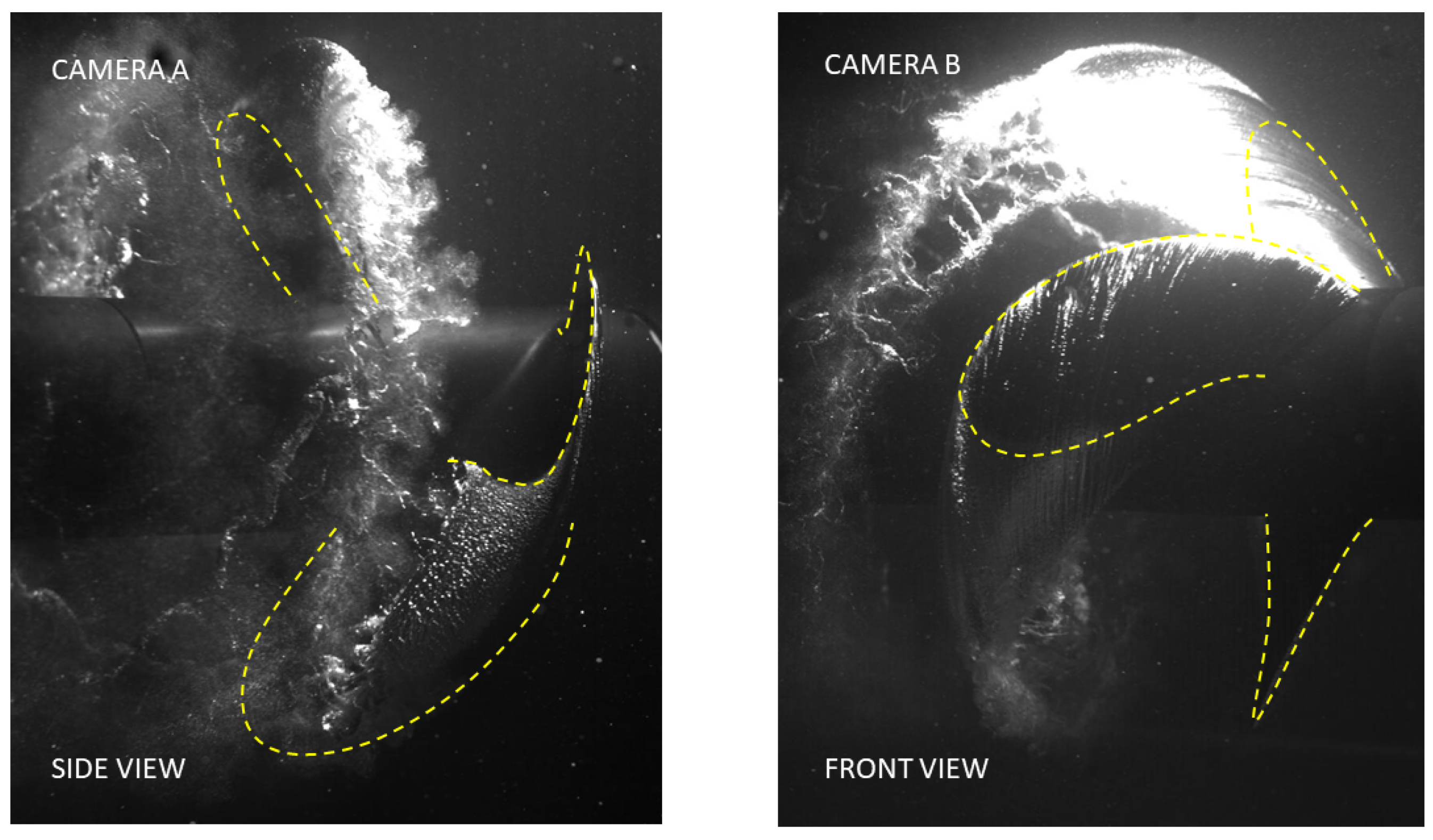
We note that, at an $r=0.7R$ radius, a steady cavity develops in plane 3 for $\sigma =1.5$ and steadily increases its angular span along X. The data in plane 6 reveal that, at $\sigma =7.2$, a drop in the number of acquired samples takes place within the range 100° < $\theta$ < 130° approximately, down to nearly 40% compared to the undisturbed flow regions. A comparison to the high-speed visualizations in Figure 4 suggests that this drop is associated with intermittent, cloud-like cavitation stemming from the blade tip. At $\sigma =1.5$, the vapor cavity extends beyond the propeller trailing edge, as plane 6 is located downstream of the propeller (see Figure 1).

By repeating this procedure for all the radial positions in the acquisition database, it is, therefore, possible to estimate the cavity size at each of the six investigated planes. Figure 9 shows the cavity thickness, defined as the elevation from the blade surface, estimated at each acquisition plane for $J=0.7$, $\sigma =1.5$, along with a three-dimensional representation of the reconstructed cavity surface. The measurement uncertainty is related to the slot size resolution, as explained in Section 2, and is shown as error bars.

We point out that this is a steady-state reconstruction, and acquisitions on the six planes were not carried out simultaneously. Additionally, the cavity region was estimated based on a zero-sample criterion, i.e., a grid point was deemed to belong to the cavity if no data were recorded during the acquisition time window. This means that a location in the flow where cavitation is fluctuating or intermittent over time is not assessed by the present approach. Only the regions where the cavity is steadily present can be characterized. However, this reconstruction is fully consistent with the mean flow phase-locked with the propeller, which is addressed in the following.

3.3. Flow Fields at Constant J, Variable $\sigma$

In this section, we present the average velocity field of the axial, radial, and tangential components, respectively $V_a$, $V_r$, and $V_t$ at planes 3 to 6 (see Table 1) and advance coefficient $J=0.7$. We compared the cavitation-free flow to the super-cavity flow to gain insight into the flow alteration induced by the onset of the specific cavitation pattern. The velocity components were made non-dimensional by the free-stream speed $U_0$. For the sake of conciseness, we focused our analysis on planes 3 to 6 since, upon preliminary analysis, planes 1 and 2 did not show a noticeable modification of the flow features. 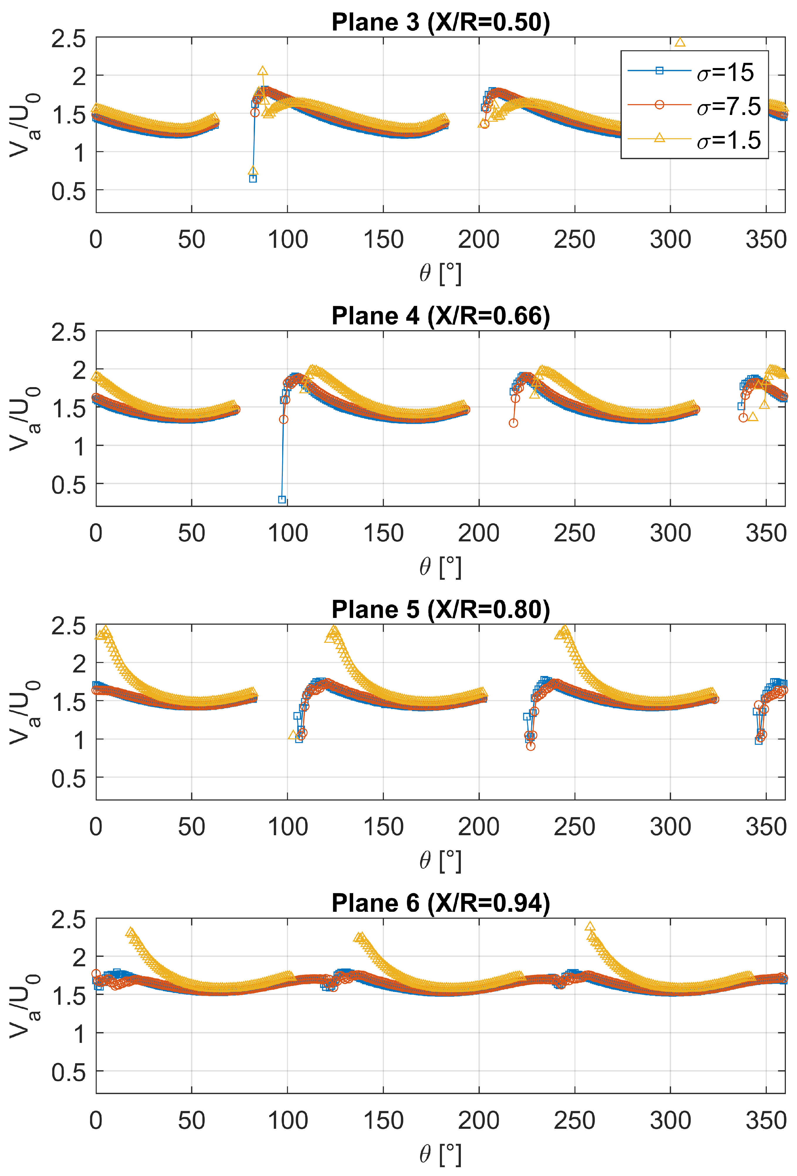In Figure 10 and Figure 11, the trend of the axial velocity $V_a$ is shown along a circular path at radii $r=0.7R$ and $r=1.0R$, respectively, from plane 3 (top) to 6 (bottom) for the three tested cavitation numbers. Uncertainty, as described in the previous section, is also reported.

At $r=0.7R$, a non-negligible difference between the cavitation-free and $\sigma =7.3$ cases was observed for plane 5, whereas in planes 3 and 4, the two curves were very similar. In plane 5, the peak axial velocity is slightly reduced for $\sigma =7.3$, and the velocity increase within the interval 225° < $\theta$ < 240° features a lower slope. This behavior is more evident in plane 6 for $\sigma =7.3$, where the velocity profile appears flatter than for the cavitation-free condition in the same $\theta$ range. As this region corresponds to the flow region on the suction side of the propeller’s blade, it was observed that even the onset of mild cavitation determined a weakening of the velocity gradients induced by the blade passage.

On the other hand, the development of the cavity for $\sigma =1.5$ markedly affects the axial velocity profiles. Despite the limited size of the cavity in plane 3, which is below 2 mm in thickness according to the data shown in Figure 9, the velocity gradient in the range 200° < $\theta$ < 225° appears strongly reduced. In fact, compared to the cavitation-free and $\sigma =7.3$ cases, where the peak axial velocity is reached at approximately $\theta$ = 200°, the peak is attained at $\theta$ = 225° in the presence of the cavity and is also reduced to $1.6U_0$ compared to the $1.8U_0$ value of the other cases.

Interestingly, the velocity profile undergoes a marked alteration in plane 4, where the cavity size is nearly three-times that found in plane 3, with a peak velocity exceeding the other cases by $0.1U_0$ and a comparable gradient in the rising phase. This trend reaches its peak in plane 5. The cavity presence induces a steep rise (occurring within 4°) of the axial velocity on the suction face of the blades, which peaks at $2.5U_0$. This is, in turn, associated with a fast descent, at the end of which $V_a$ levels at the same values as the other conditions. Due to the super-cavity formation, the effect persists also in plane 6, although slightly weakened, with a peak velocity not exceeding $2.3U_0$.

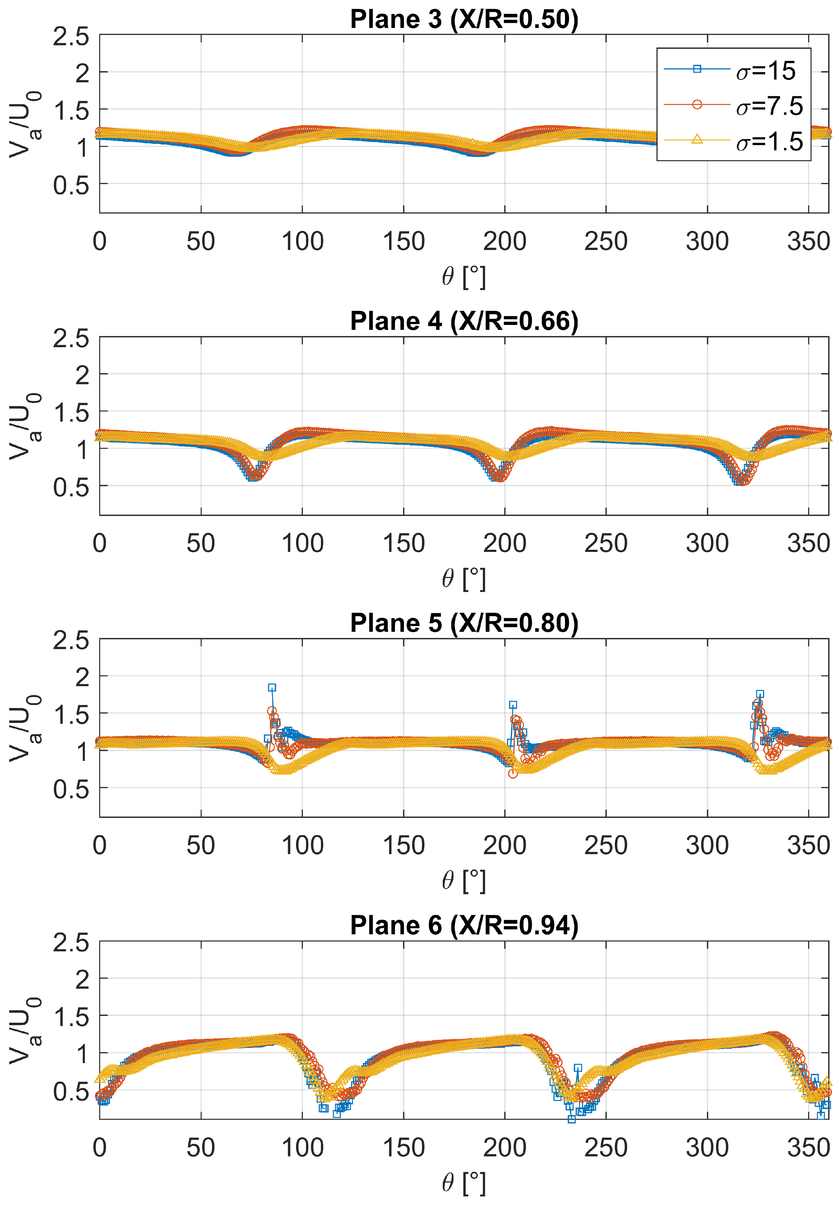
The analysis at the radial position $r=1.0R$, reported in Figure 11, shows the impact of the cavity development on more-peripheral flow regions. Furthermore, it allows the investigation of the interactions between the cavity and the tip-vortex structure that forms in this region. Consistent with the situation at $r=0.7R$, the cavitation-free and $\sigma =7.3$ cases are very similar for plane 3, whereas a flatter profile is reported for $\sigma =1.5$. This behavior is conserved at more downstream positions: the curves’ trend reveals a smoother behavior of $V_a$ under full cavitation in the angle interval matching the blade passage (approximately 205° < $\theta$ < 220° in plane 4), compared to the cavitation-free conditions, where the spatial velocity fluctuations due to the tip-vortex are evident. The impact of the cavity on the tip-vortex region is evident in planes 5 and 6. While the cavitation-free case features a strong peak at $\theta$ = 205°, the $\sigma =7.3$ case shows a lower peak followed by a short region characterized by $V_a<U_0$. We note that, for full-cavitation conditions, the axial velocity never exceeds the free-stream speed. In plane 6, the inspection of the cavitation-free case reveals a small tip-vortex region for 238° < $\theta$ < 240°, which vanishes at $\sigma =7.3$. For $\sigma =1.5$, the velocity profile features a local maximum at approximately $\theta$ = 245°. The role of the cavity in the modification of the flow in the blade tip region is, thus, evident and was further investigated via analysis of the velocity fields. An overview of the $V_a$ fields, provided in Figure 12, reveals that slight leading edge and tip-vortex cavitation have a moderate impact on the axial flow field structure, whereas the presence of the full cavity at $\sigma =1.5$ modifies the flow field dramatically.

Starting from plane 3, the axial flow field undergoes substantial changes at $\sigma =1.5$, although the cavity size does not exceed, on average, 25% of its maximum size. The inner region ($r<0.7R$) features a slight increase in axial flow velocity in the accelerated flow area, which appears limited to this region. As a consequence, the outer region, around $r=1.0R$, features smoother gradients compared to the other cases. As the cavity size increases (see plane 4), the axial flow acceleration discussed in Figure 10 for $r=0.7R$ is explained by the observation of a more-pronounced displacement of the accelerated flow region towards the inner radii. In particular and compared to the cavitation-free case, the accelerated flow area, which is defined as the region for which $V_a>1.5U_0$ holds, shrinks from $r<0.9R$ to $r<0.8R$. On the other hand, the peak velocity reaches the value of $U_0=2$.

In plane 5 and clearly outlined by the blank area, the cavity volume increases, and the flow region close to the cavity boundaries undergoes an increase up to $2.5U_0$. The smoothness of the velocity peaks previously reported at $r=1.0R$ is here better explained with the data in plane 5. The strong local gradients observed at $\sigma =15$ are compared to a gradual decrease for $\sigma =7.3$ and substantial modifications at $\sigma =1.5$. Under fully developed cavitation, the velocity peaks in this region vanish and are replaced by a deceleration zone that extends to approximately $r=0.8R$, where the flow acceleration begins due to the cavity occurrence. It appears that the impact of the cavity on the flow field is not limited to the locations where the cavity develops, but extends to other flow areas. The cavity extending beyond the propeller trailing edge, as observed through the visualizations, is here confirmed by the results in plane 6 where a no-data region is clearly visible. The axial inter-blade flow features an increase up to $1.6U_0$ in the region close to the hub, compared to $1.5U_0$ at the same location in the flow for non-cavitating conditions. Insight into the interactions between the cavity and the tip-vortex is given by the analysis of the velocity maps in plane 6. The presence of a steady tip-vortex cavity is noticeable for the cavitation-free case and can be identified by the small blank areas spanning a 4° range. Starting at $\sigma =7.3$, this small cavitation region is no longer detectable, whereas the tip-vortex trace appears stretched and elongated in the tangential direction. For $\sigma =1.5$, the trace of the tip-vortex is not detectable and is replaced by an isolated accelerated region. This complex behavior is possibly associated with the non-trivial shape of the cavity in the region $0.8R<r<1.0R$. It appears that the formation of a steady cavity reaching further than the propeller blade size works as an accelerator by narrowing the inter-blade section.

The normalized fields of the tangential component of velocity $V_t$ are shown in Figure 13 for planes 3 to 6. Compared to the non-cavitating conditions, the tip region at $\sigma =7.3$ is affected by a decrease of the tangential component at every downstream position. In particular, in planes 3 and 4, the positive and negative $V_t$ regions at the tip appear to be weaker than the $\sigma =15$ case. In plane 5, the region $V_t<0$ has nearly vanished, while a $V_t>0$ area on the suction side of the blade can be identified. In plane 6, the velocity field at $\sigma =7.3$ is characterized by a tip region with $V_t>0$. This is in stark contrast to the free-cavitation conditions. As discussed before, a small blank area of steady cavitation is associated with the tip-vortex, and this area is surrounded by two $V_t$ regions of opposite sign. This scenario is confirmed by the development of tip-vortex cavitation, as visualized in Figure 4. At the most-downstream plane, the trace of the rolling shear layers stemming from the propeller’s blade trailing edge is also visible. For fully cavitating conditions, several changes in the flow field can be noticed. Starting at plane 3, the $V_t$ contour map appears markedly changed. The overall value of $V_t$ does not drop below $-0.1U_0$ compared to the $-0.8U_0$ minimum value found in the tip region at $\sigma =7.3$. The swirling motion induced by the tip structures is dampened by the cavity at its early stage of development. The inner radii feature an overall increase of the tangential component, in particular towards the pressure side of the blades. In plane 4, the trace of the tip-vortex (highlighted by a red circle) is not visible, while the $V_t$ map in the inter-blade region appears more homogeneous. This finding reveals a scenario similar to that of the axial component discussed before. As the cavity grows in size, with a thickness more homogeneously distributed along the tangential direction, the flow field components tend to have a more-homogeneous trend. In this respect, the trace of the shear layer roll-up visible for the other cases is merged into the acceleration zone in the $\sigma =1.5$ case. At the most-downstream location and for the fully developed cavitation case, the trace of the trailing edge shear layers gives way to the cavity while the rest of the velocity field shows no particular pattern. The tangential velocity increase appears limited to the areas close to the cavity surface and the propeller’s hub. On the other hand, the areas towards the blades’ pressure side display a distribution similar to the $\sigma =7.3$ condition. In the tip region, the cavity presence causes the $V_t$ value not to exceed $0.2U_0$ compared to $0.8U_0$ of the $\sigma =7.3$ case in the same region. The cavity’s presence has a dampening effect on the local $V_t$ gradients associated with the tip-vortex at the outer radii. This effect is compensated by an increase of the tangential component in the inner regions.

Further insight into the role played by the cavity in accelerating the inter-blade flow is given by the plots of Figure 14, where the $V_a$ increment between cavitating ($\sigma =1.5$) and non-cavitating flow ($\sigma =15$) is shown in three planes. The increment is normalized versus the free-stream speed.

These results confirm that, as the cavity develops (see the plots for plane 4, middle picture) and up to approximately half of the propeller radius, the region close to the hub is characterized by an axial flow acceleration, ranging from nearly $0.4U_0$ to $0.7U_0$, in the area adjacent to the cavity. In plane 5 and at $r=0.6R$, the flow right above the cavity experiences the maximum $V_a$ increment, reaching $0.9U_0$. The axial flow increment persists also downstream of the propeller in plane 6, with a maximum increment of $0.6U_0$. These findings show that, at the location of maximum cavity thickness, the axial flow acceleration is still present, albeit weakened, in the near-wake. The region near the blade tips exhibits a different trend, with local regions of both an increase and decrease of the axial velocity. This is explained with the help of high-speed visualizations; see Figure 4, Figure 5 and Figure 6. The development of an extended cavity is concurrent with the disappearance of the tip-vortex structure.

In a similar manner, we report the increment of $V_t$ in Figure 15. The reduced development of the tip-vortex occurring at this $\sigma$ is confirmed by the tangential acceleration/deceleration pattern in the tip region for planes 3 to 5. In plane 6, a different pattern of a tangential velocity increment is observed. The outer region surrounding the cavity along the radial direction undergoes a strong decrease, with a $-0.7U_0$ peak level compared to $-0.4U_0$ for $\sigma =7.3$. This observation shows that, in the near-wake, the cavity impact on the flow tangential component is stronger. Interestingly, the tangential velocity is reported to increase in the inner inter-blade region, particularly in plane 4, indicating that the flow swirl generated by the propeller is stronger at the inner radii. Nevertheless, for radii $r<0.7R$, the effect of the cavity on the tangential velocity increase is different from that on the axial component. The peak increment of $V_t$ is about $0.4U_0$ and $0.5U_0$ at $r=0.6R$ for planes 5 and 6, respectively. While the axial increment peak was attained in plane 5 and was followed by a decrease in plane 6, this trend is reversed for the $V_t$ component for which the increment keeps growing, showing that the cavity interacts with the flow in a complex way.

These findings were usefully compared to the propeller performance data, which were obtained experimentally. With T, Q, n, and $\rho$ being the thrust, torque, rotation rate, and water density at 21 °C, respectively, the corresponding thrust coefficient $K_t=T/\left(\rho n^2{D}^4\right)$, torque coefficient $K_q=Q/\left(\rho n^2{D}^5\right)$, and efficiency $\eta =J{K}_t/\left(2\pi K_q\right)$ are calculated and collected in

Table 4. Propeller performance at $J=0.7$.

$\mathit{\sigma }$	${\mathit{K}}_{\mathit{t}}$	${\mathit{K}}_{\mathit{q}}$	$\mathit{\eta }$
15	0.40	0.09	0.51
7.3	0.40	0.09	0.50
1.5	0.31	0.08	0.45

for $J=0.7$. The results show that light leading-edge cavitation does not affect the propeller performance, whereas the extended cavity at $\sigma =1.5$ is responsible for a loss of five percentage points of efficiency, corresponding to a relative loss of efficiency of approximately 11%. It appears that the presence of the extended cavity works as a local axial and tangential flow accelerator, as evinced from the velocity field data, by increasing the momentum ejection through the propeller. This increased momentum partly compensates the expected drop in performance.

4. Conclusions

The inter-blade flow around a super-cavitating propeller was investigated in a cavitation tunnel facility via high-speed imaging and laser Doppler velocimetry (LDV) at different loading conditions. A range of cavitating stages was observed, from tip-vortex cavitation to full cavity development. The onset of a steady cavity extending beyond the trailing edge was reported for the highest loading conditions ($J=0.7$), preceded by inner blade surface cavitation.

The analysis of the axial velocity profiles at radii $r=0.7R$ and $r=1.0R$ highlights the impact of the developing cavity on the flow field in different regions. At $r=0.7R$ and for $\sigma =7.3$, the axial velocity profile is characterized by weaker gradients along the tangential direction on the suction side of the propeller’s blades, compared to the cavitation-free case, particularly at downstream locations, i.e., at $X/R=0.66$. For $\sigma =1.5$, the axial velocity gradients are reduced starting at $X/R=0.50$. At the outer radius $X/R=1.0$, velocity peaks due to the tip-vortex are diminished at $\sigma =7.3$ and vanish at $\sigma =1.5$. The analysis of the axial and tangential velocity maps shows that the zone of axial flow acceleration shifts towards the inner radii as the cavity grows in size. Simultaneously, the axial flow reaches a peak of $2.5U_0$, specifically at $X/R=0.80$. Under fully developed cavitation conditions, the axial flow acceleration persists at $X/R=0.94$, even though it drops from a $0.9U_0$ increase to $0.6U_0$ compared to the cavitation-free case. This behavior is not observed for the tangential component, which steadily increases even in the near-wake plane, reaching its maximum increment of $0.5U_0$ compared to the $\sigma =15$ case. Due to the tip-vortex forming at $\sigma =15$ in the near-wake, the tip-vortex region exhibits a small cavity that vanishes at $\sigma =1.5$, where a marked reduction of both axial and tangential gradients is found. Overall, a reduced development of the tip-vortex is observed at $\sigma =1.5$.

Our results point out that extended cavitation is characterized by a long, enveloping cavity and a relevant inter-blade axial and tangential flow acceleration. A reliable methodology for the estimate of the cavity extension and volume was presented and applied to the data. The proposed methodology exploits the ability of LDV to access inter-blade regions and demonstrates its robustness against harmful light reflections, which typically occur when employing laser light in cavitating flows. The methodology provides a quantitative estimate of the size of the flow regions that are cavitating steadily over the acquisition window and is, therefore, compatible with a phase-locked reconstruction of the mean flow. The methodology, however, was not validated for the assessment of unsteady cavitation, as it may not capture the associated flow phenomena with the current analysis criteria.

References

1. Franc, J.P.; Michel, J.M. Fundamentals of Cavitation; Springer Science & Business Media: Berlin/Heidelberg, Germany, 2006; Volume 76. [Google Scholar]
2. Barr, R.A. Supercaviting and superventilated propellers. Soc. Nav. Archit. Mar. 1970, 78, 417–451. [Google Scholar]
3. Kirschner, I.N.; Kring, D.C.; Stokes, A.W.; Fine, N.E.; Uhlman, J.S., Jr. Control strategies for super-cavitating vehicles. J. Vib. Control 2002, 8, 219–242. [Google Scholar] [CrossRef]
4. Park, S.; Rhee, S.H. Computational analysis of turbulent super-cavitating flow around a two-dimensional wedge-shaped cavitator geometry. Comput. Fluids 2012, 70, 73–85. [Google Scholar] [CrossRef]
5. Ahn, B.K.; Lee, T.K.; Kim, H.T.; Lee, C.S. Experimental investigation of super-cavitating flows. Int. J. Nav. Archit. Ocean Eng. 2012, 4, 123–131. [Google Scholar] [CrossRef]
6. Li, X.; Wang, G.; Zhang, M.; Shyy, W. Structures of super-cavitating multiphase flows. Int. J. Therm. Sci. 2008, 47, 1263–1275. [Google Scholar] [CrossRef]
7. Kamiirisa, H.; Aoki, D. Development of super-cavitating propeller for outboard motors. In Proceedings of the Second International Symposium on Cavitation, Tokyo, Japan, 5–7 April 1994; pp. 5–7. [Google Scholar]
8. Ukon, Y.; Kudo, T. Design of high performance super-cavitating propellers based on a vortex lattice method. Br. Marit. Technol. 1995, 175, 47. [Google Scholar]
9. Young, Y.; Kinnas, S. Analysis of super-cavitating and surface-piercing propeller flows via BEM. Comput. Mech. 2003, 32, 269–280. [Google Scholar] [CrossRef]
10. Alves Pereira, F.; Salvatore, F.; Di Felice, F. Measurement and modeling of propeller cavitation in uniform inflow. J. Fluids Eng. 2004, 126, 671–679. [Google Scholar] [CrossRef]
11. Alves Pereira, F.; Di Felice, F.; Salvatore, F. Propeller cavitation in non-uniform flow and correlation with the near pressure field. J. Mar. Sci. Eng. 2016, 4, 70. [Google Scholar] [CrossRef]
12. Felici, A.; Di Felice, F.; Alves Pereira, F. Measurement of the cavitation pattern by two non-intrusive techniques: Laser imaging and ultrasound pulsed echography. Exp. Fluids 2013, 54, 1482. [Google Scholar] [CrossRef]
13. Konno, A.; Wakabayashi, K.; Yamaguchi, H.; Maeda, M.; Ishii, N.; Soejima, S.; Kimura, K. On the mechanism of the bursting phenomena of propeller tip vortex cavitation. J. Mar. Sci. Technol. 2002, 6, 181–192. [Google Scholar] [CrossRef]
14. Aktas, B.; Atlar, M.; Turkmen, S.; Shi, W.; Sampson, R.; Korkut, E.; Fitzsimmons, P. Propeller cavitation noise investigations of a research vessel using medium size cavitation tunnel tests and full-scale trials. Ocean Eng. 2016, 120, 122–135. [Google Scholar] [CrossRef]
15. Ji, B.; Luo, X.; Peng, X.; Wu, Y.; Xu, H. Numerical analysis of cavitation evolution and excited pressure fluctuation around a propeller in non-uniform wake. Int. J. Multiph. Flow 2012, 43, 13–21. [Google Scholar] [CrossRef]
16. Ji, B.; Luo, X.; Wu, Y.; Peng, X.; Xu, H. Partially-Averaged Navier–Stokes method with modified k–ε model for cavitating flow around a marine propeller in a non-uniform wake. Int. J. Heat Mass Transf. 2012, 55, 6582–6588. [Google Scholar] [CrossRef]
17. Kubota, A.; Kato, H.; Yamaguchi, H.; Maeda, M. Unsteady structure measurement of cloud cavitation on a foil section using conditional sampling technique. J. Fluids Eng. 1989, 111, 204–210. [Google Scholar] [CrossRef]
18. Wu, Q.; Wang, C.C.; Huang, B.; Wang, G.Y.; Cao, S.L. Measurement and prediction of cavitating flow-induced vibrations. J. Hydrodyn. 2018, 30, 1064–1071. [Google Scholar] [CrossRef]
19. Peng, X.x.; Xu, L.h.; Liu, Y.w.; Zhang, G.p.; Cao, Y.t.; Hong, F.w.; Yan, K. Experimental measurement of tip vortex flow field with/without cavitation in an elliptic hydrofoil. J. Hydrodyn. Ser. B 2017, 29, 939–953. [Google Scholar] [CrossRef]
20. Simanto, R.; Hong, J.W.; Ahn, B.K.; Jeong, S.W. Experimental investigation on tip vortex cavity deformation and flow dynamics using high-speed imaging and laser Doppler velocimetry measurements. Phys. Fluids 2023, 35, 107104. [Google Scholar] [CrossRef]
21. Boulon, O.; Callenaere, M.; Franc, J.P.; Michel, J.M. An experimental insight into the effect of confinement on tip vortex cavitation of an elliptical hydrofoil. J. Fluid Mech. 1999, 390, 1–23. [Google Scholar] [CrossRef]
22. Stella, A.; Guj, G.; Di Felice, F. Propeller wake flowfield analysis by means of LDV phase sampling techniques. Exp. Fluids 2000, 28, 1–10. [Google Scholar] [CrossRef]
23. Alves Pereira, F.; Capone, A.; Di Felice, F. Flow field and vortex interactions in the near wake of two counter-rotating propellers. Appl. Ocean Res. 2021, 117, 102918. [Google Scholar] [CrossRef]
Figure 1. Overall points’ grid. Red lines highlight the points scanned by the LDV probe. The propeller cylindrical coordinate system and corresponding velocity field components are also shown.
Jmse 12 00243 g001
Figure 2. Sketch of the experimental setup. The LDV head moves along the X L , Y L , and Z L directions (pointing upwards) to acquire data on the corresponding X, Y, and Z directions of the propeller’s coordinate system; see Figure 1.
Jmse 12 00243 g002
Figure 3. Visualization of blade tip cavitation. J = 1.0 and σ = 7.2 . Snapshots of front and side camera views. The blade edge is outlined by the dashed line.
Jmse 12 00243 g003
Figure 4. Visualization of leading edge cavitation. J = 0.7 and σ = 7.3 . Snapshots of front and side camera views.
Jmse 12 00243 g004
Figure 5. Visualization of mid chord and tip cavitation. J = 1.0 and σ = 1.5 . Snapshots of front and side camera views.
Jmse 12 00243 g005
Figure 6. Visualization of fully developed cavitation (super-cavity). J = 0.7 and σ = 1.5 . Snapshots of front and side camera views.
Jmse 12 00243 g006
Figure 7. Normalized number of samples S versus angular position θ at J = 0.7 for different σ values. r = 0.7 R , plane 5 ( X / R = 0.80 ).
Jmse 12 00243 g007
Figure 8. Normalized number of samples S versus angular position θ at J = 0.7 for different σ values. r = 0.7 R , planes 1 to 6. Due to the three-blade symmetry, only a 180° angle span is shown.
Jmse 12 00243 g008
Figure 9. Cavity thickness estimate at different planes for J = 0.7 and σ = 1.5 (left) and cavity surface three−dimensional representation (right).
Jmse 12 00243 g009
Figure 10. Average axial velocity at J = 0.7 , r = 0.7 R . Planes 3 to 6 (topbottom).
Jmse 12 00243 g010
Figure 11. Average axial velocity at J = 0.7 , r = 1.0 R . Planes 3 to 6 (topbottom).
Jmse 12 00243 g011
Figure 12. Average axial velocity at J = 0.7 , planes 3 (topbottom). σ = 15 (left), σ = 7.3 (middle), and σ = 1.5 (right). Blank areas highlighted by the black arrows represent the cavity in the corresponding plane.
Jmse 12 00243 g012
Figure 13. Average tangential velocity at J = 0.7 , planes 3 to 6 (topbottom). σ = 15 (left), σ = 7.3 (middle), and σ = 1.5 (right). The red circle highlights the flow region where tip−vortex development is reduced.
Jmse 12 00243 g013
Figure 14. Axial velocity component increment in cavitating conditions ( σ = 1.5 ) compared to non−cavitating ( σ = 15 ) at J = 0.7 .
Jmse 12 00243 g014
Figure 15. Tangential velocity component increment in cavitating conditions ( σ = 1.5 ) compared to non−cavitating ( σ = 15 ) at J = 0.7 .
Jmse 12 00243 g015