

Numerical Analysis of Ice–Structure Impact: Validating Material Models and Yield Criteria for Prediction of Impact Pressure

Abstract
:1. Introduction
2. Material Properties of Ice
2.1. Constitutive Equations for Ice Elasto-Plastic Behavior
2.2. Yield Criteria Models of Ice
- (1)
- Crushable Foam yield model
- (2)
- Drucker–Prager yield model
- (3)
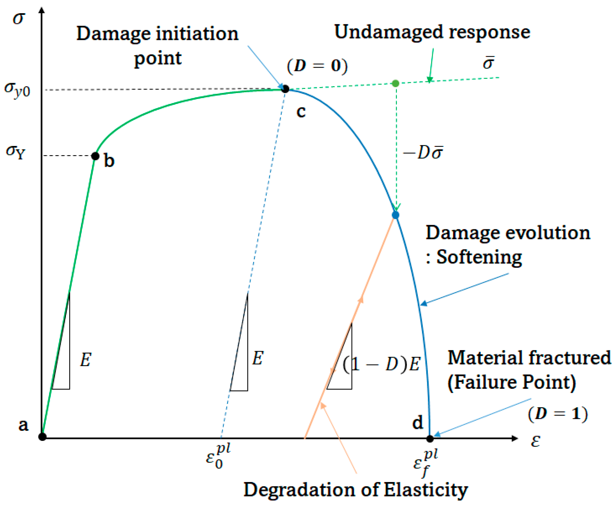
- Progressive damage model
2.3. Strain Rate Dependency of Ice: Yield Strength Ratio
3. Ice Material Calibration
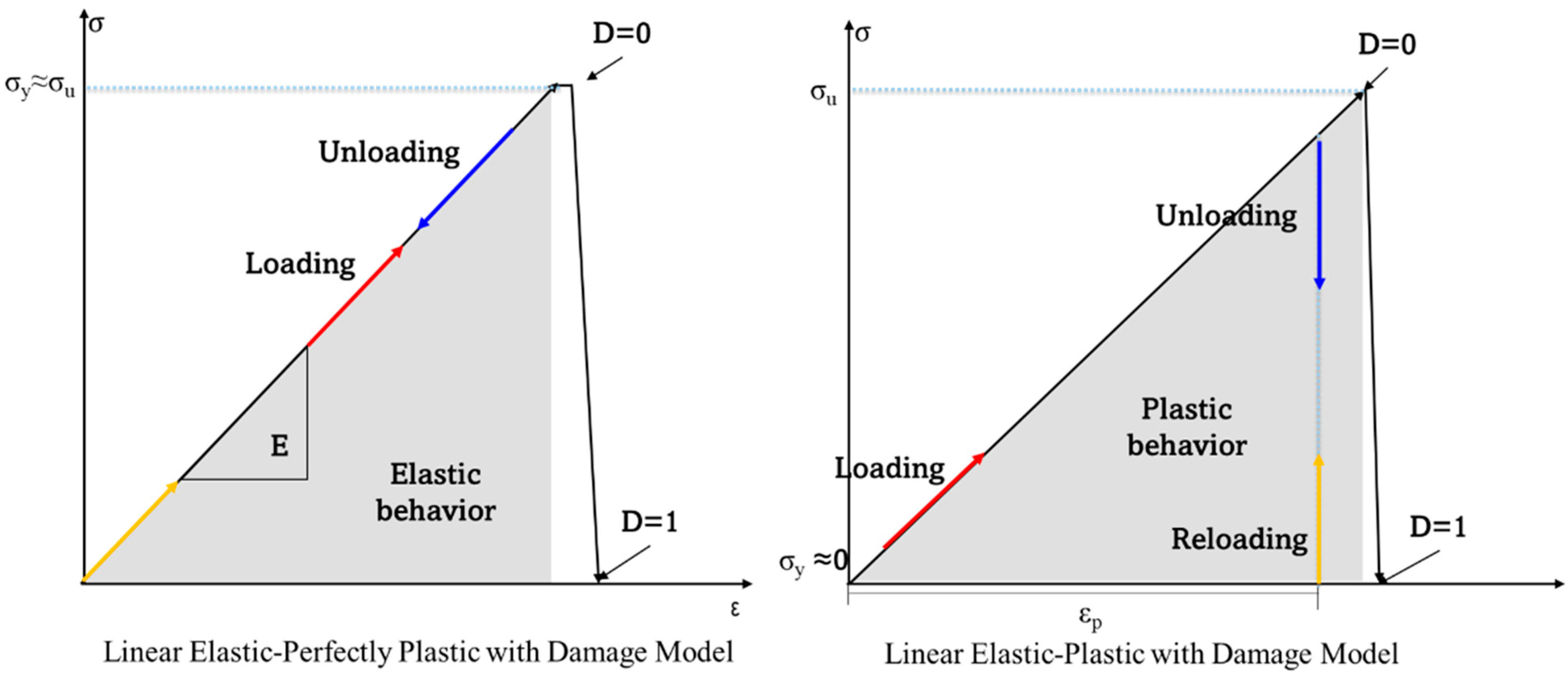
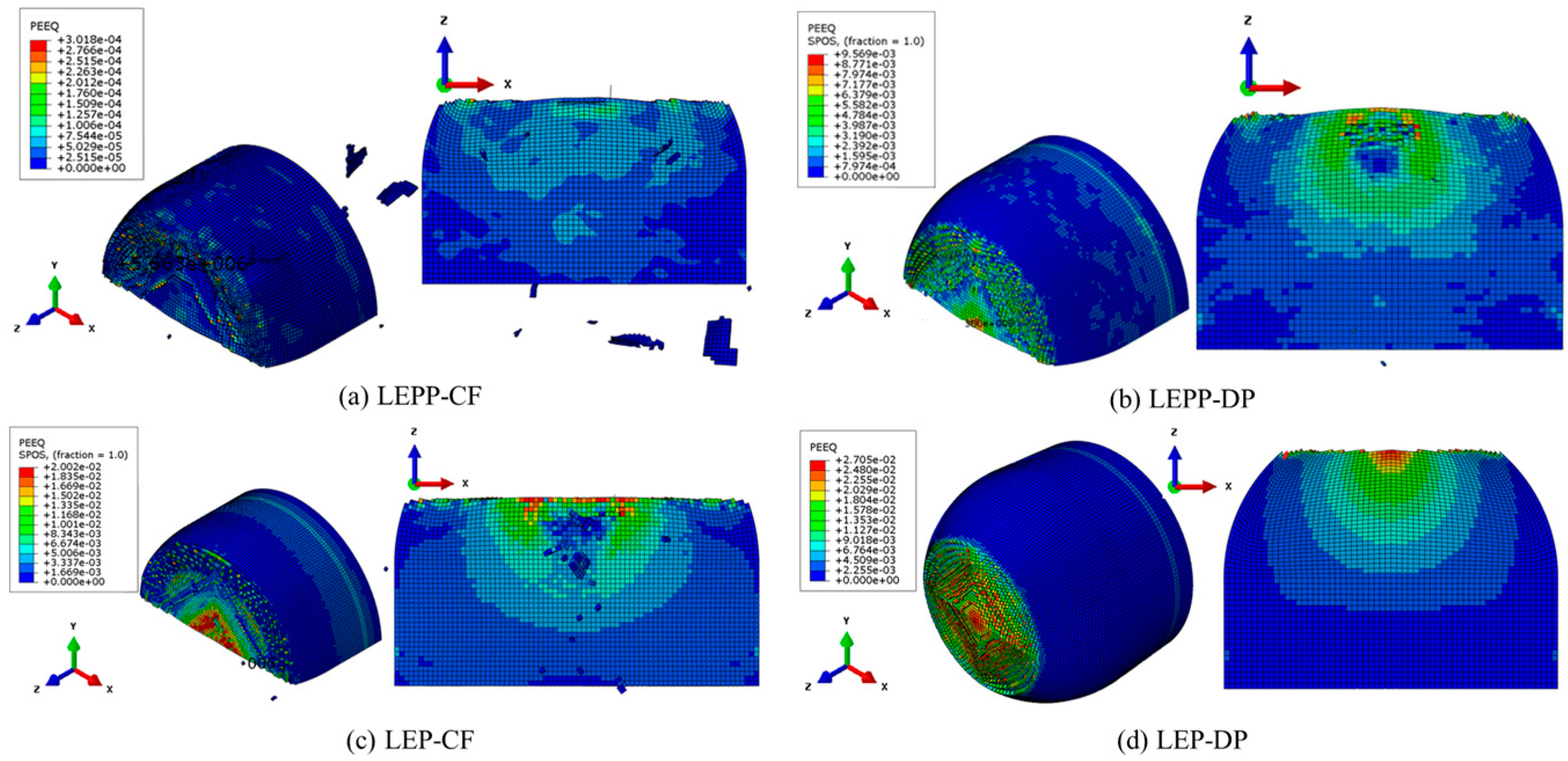
- Plastic deformation relationships: Models such as the Linear Elastic-Perfectly Plastic (LEPP) and Linear Elastic-Plastic (LEP) models define how materials behave when they exceed the elastic limit. While the LEPP model assumes that no deformation occurs beyond the yield point, the LEP model describes post-yield hardening or softening. These material plastic properties are applied to the analyses to verify their results.
- Yield criteria: The Crushable Foam (CF) and Drucker–Prager (DP) models define the conditions under which materials reach yield. The CF model simulates the collapse of cellular materials under compression, whereas the DP model models the yield of pressure-dependent materials. Given the sensitivity of ice to pressure and density, the appropriateness of these conditions was investigated.
- Strain rate dependence: In dynamic events such as collisions, strain rate affects the yield stress and failure modes of the material. Results are analyzed based on whether or not strain rate dependence is considered.
3.1. Determination of Material Model Constants
- The LEPP model: This model requires the determination of two fundamental material constants, Young’s modulus () and the yield stress (). Young’s modulus is conventionally obtained from tensile tests, whereas the yield stress is the stress point at which the material begins to undergo plastic deformation.
- The LEP model: Similar to LEPP, the LEP model requires the determination of Young’s modulus () and yield stress (). In addition, it requires the consideration of additional constants associated with the hardening model and the hardening coefficient or plastic flow rule.
- The CF model: This model requires the definition of material constants that govern the compressive behavior of foams. Key constants include density, initial strength (), and hardening coefficient. The determination of these constants is facilitated by the analysis of stress-strain curves derived from compression tests on specimens.
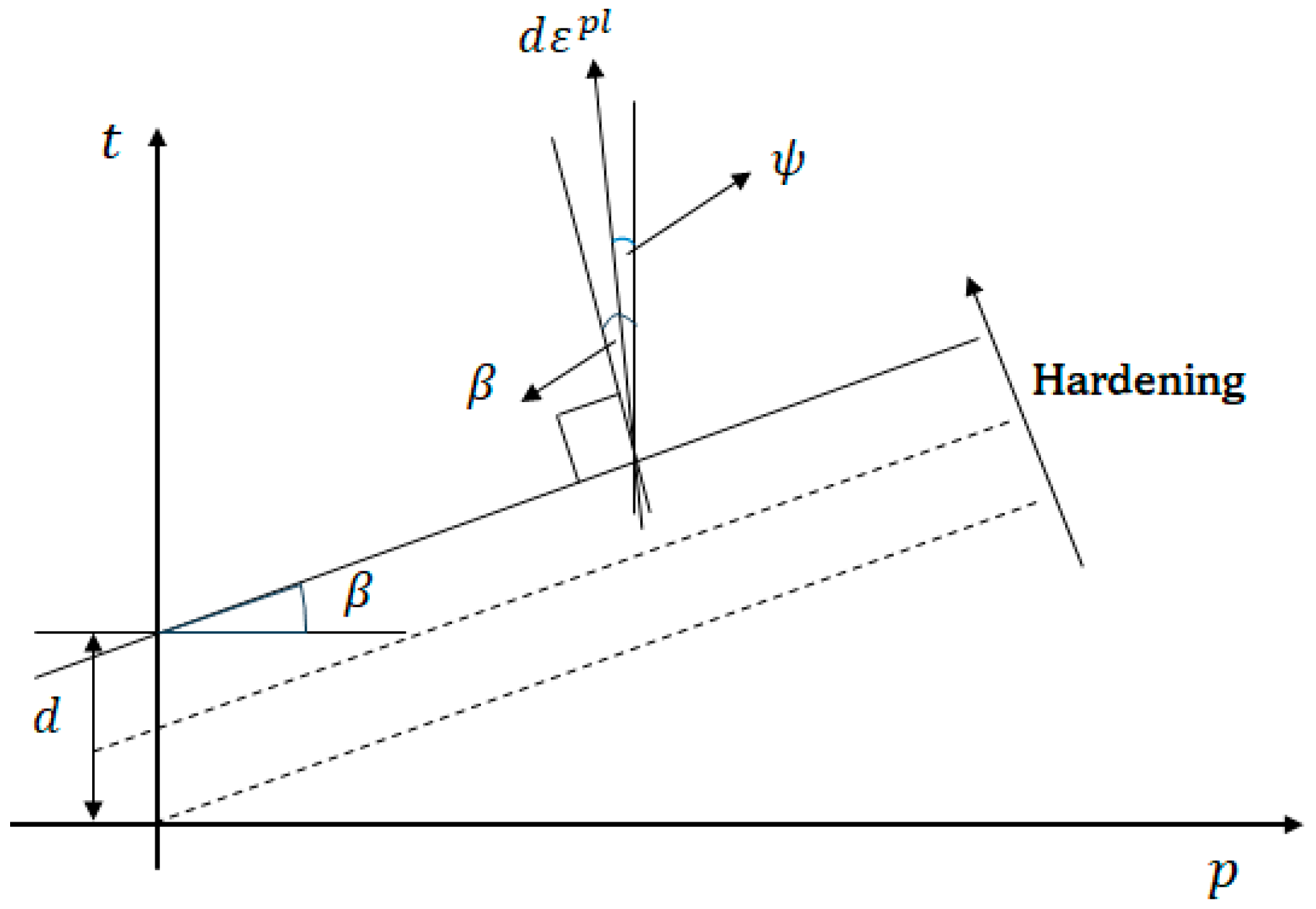
- The DP model: The DP model requires a set of constants related to the angle of internal friction (β), material cohesion (d), drag parameters such as the dilatancy angle (ψ), and constants related to the hardening rule. Typically, these constants are obtained from triaxial compression tests and should be considered in conjunction with stress paths.
- The LEPP model: The apparent elastic modulus was assumed to be 0.14 GPa. The yield stresses for the CF and DP models were set at 4.8 MPa and 3 MPa respectively. The material damage model parameters included a failure strain of 1.0 × 10⁻⁴ and an energy release rate of 15.0 J.
- The LEP model: The elastic modulus, influenced by stress and strain rate, was set to 9 GPa. Hardening constants for this model are detailed in Table 4 for both the CF and DP models, and failure strains were designated as 0.019 and 0.025, respectively, with a damage evolution energy of 15.0 J.
3.2. Finite Element Analysis Simulating Ice Compression Experiments
4. Simulation Model for the Ice–Structure Collision Experiment
- Ice yield criteria: The CF and DP models were used to model the yielding and failure behavior of ice, as described in Section 2.1.
- Contact conditions: Contact conditions were established to account for the interaction between the two objects and to calculate the load transferred from the ice to the structure. For the contact between ice elements and plates, hard contact and tie conditions are applied. The tie conditions were applied to ice and holder, and steel plate and jig, respectively.
- Element with reduced integration: Reduced integration was used to establish the stiffness matrix to enhance the computational efficiency, along with the selection of the hourglass control.
- Time increment: In accordance with the Courant–Friedrichs–Lewy (CFL) condition, the time increment () for the explicit finite element analysis was determined. The time increment was calculated using the formula: , where is the size of the smallest element within the mesh. The term represents the material’s dilatational wave speed (P-wave speed), which is the function of the material’s mechanical properties. For isotropic material, was calculated using the formula , where is the elastic modulus, is the Poisson’s ratio, and is the density of the material.
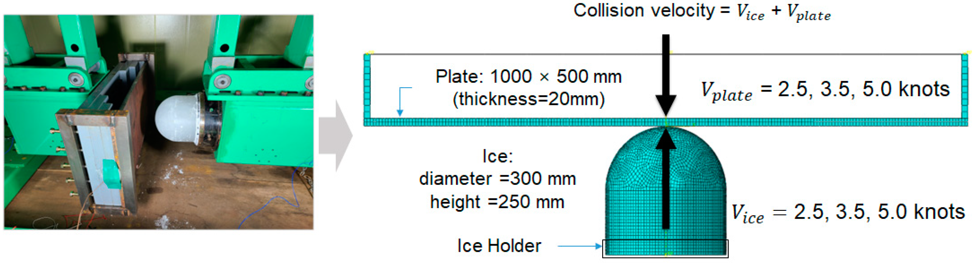
4.1. Overview of the Ice–Structure Collision Simulation Model
4.2. Mesh Convergence Test
4.3. Collision Analysis Reflecting Quasi-Static Compressed Material Model
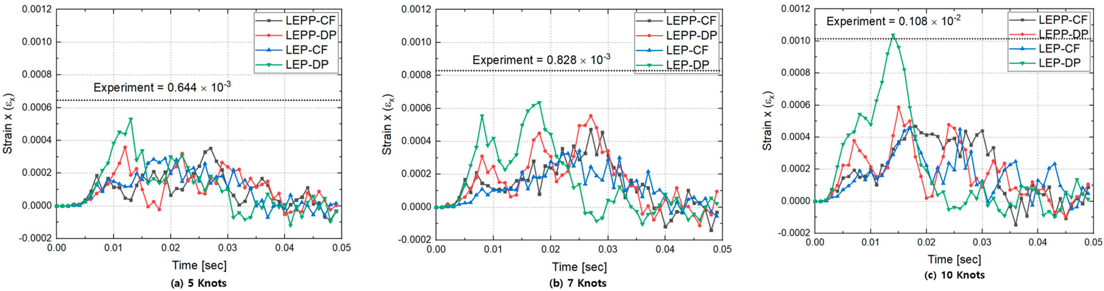
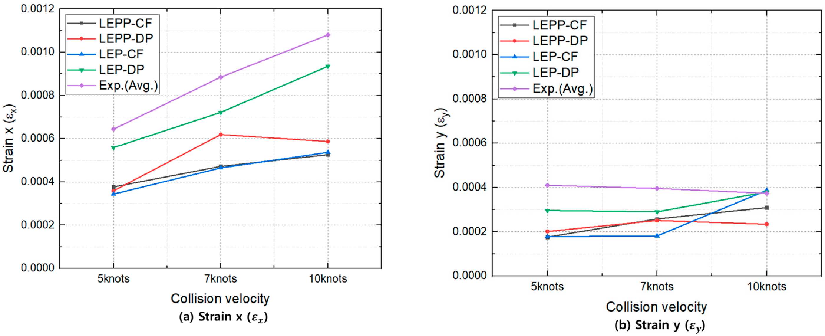
- Predicted strains on steel plate
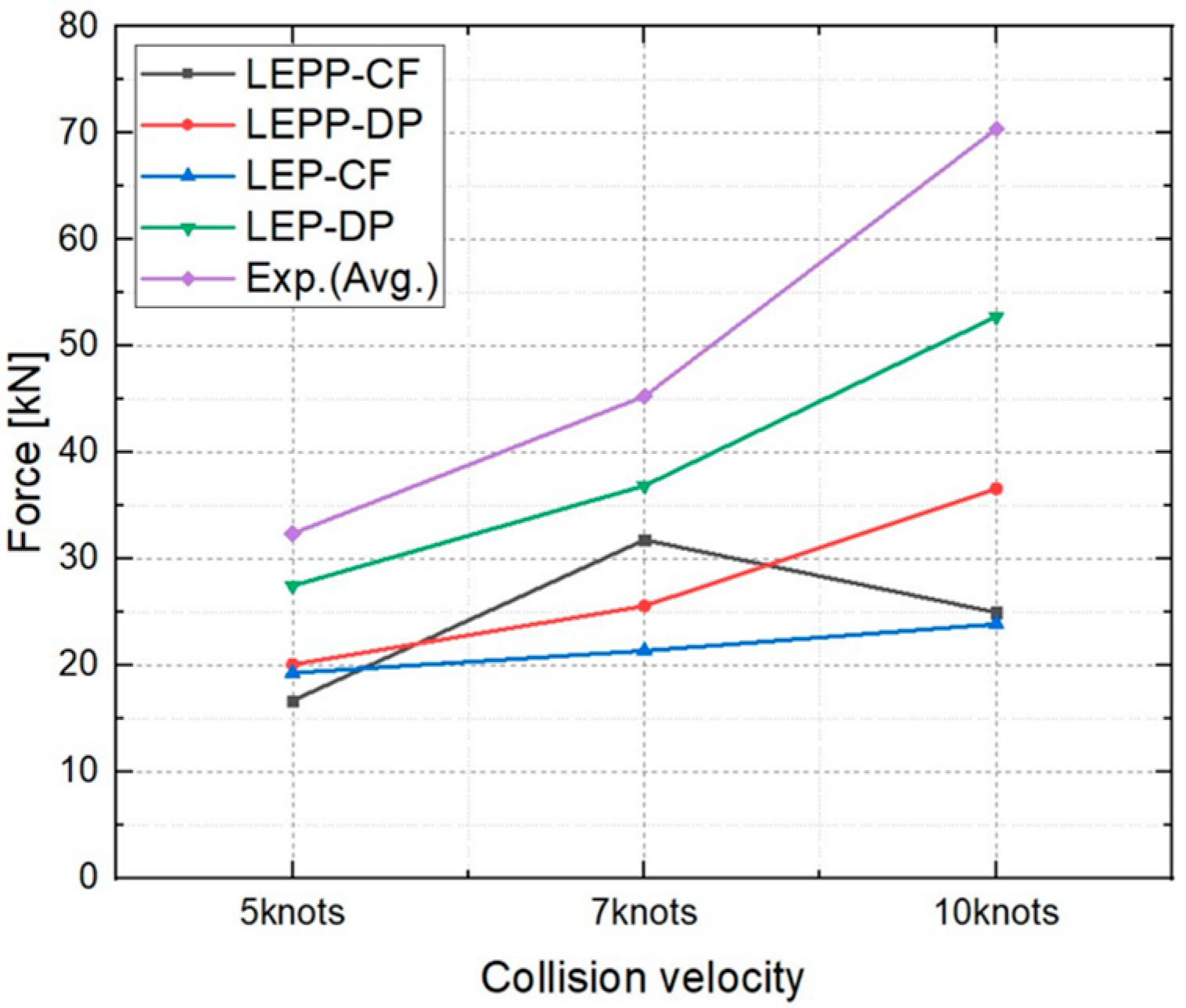
- Ice collision force prediction results
4.4. Collision Analysis Reflecting Yield Ratio according to Strain Rate
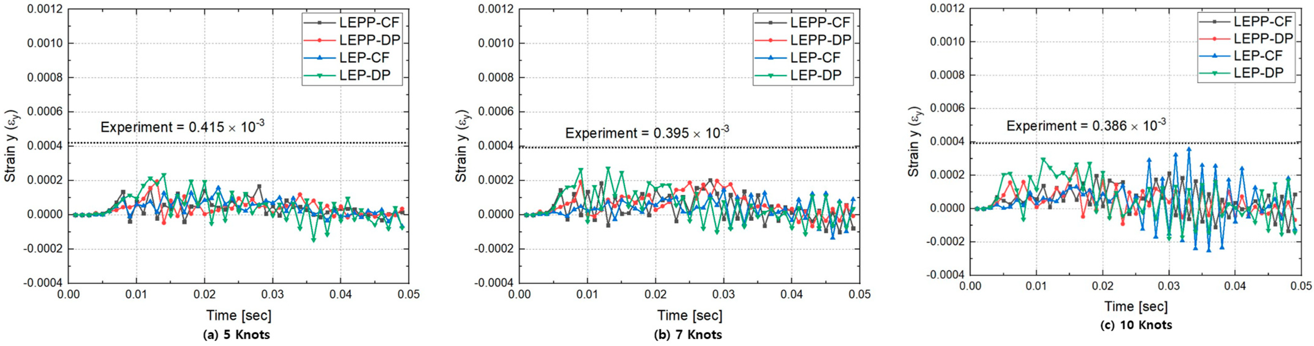
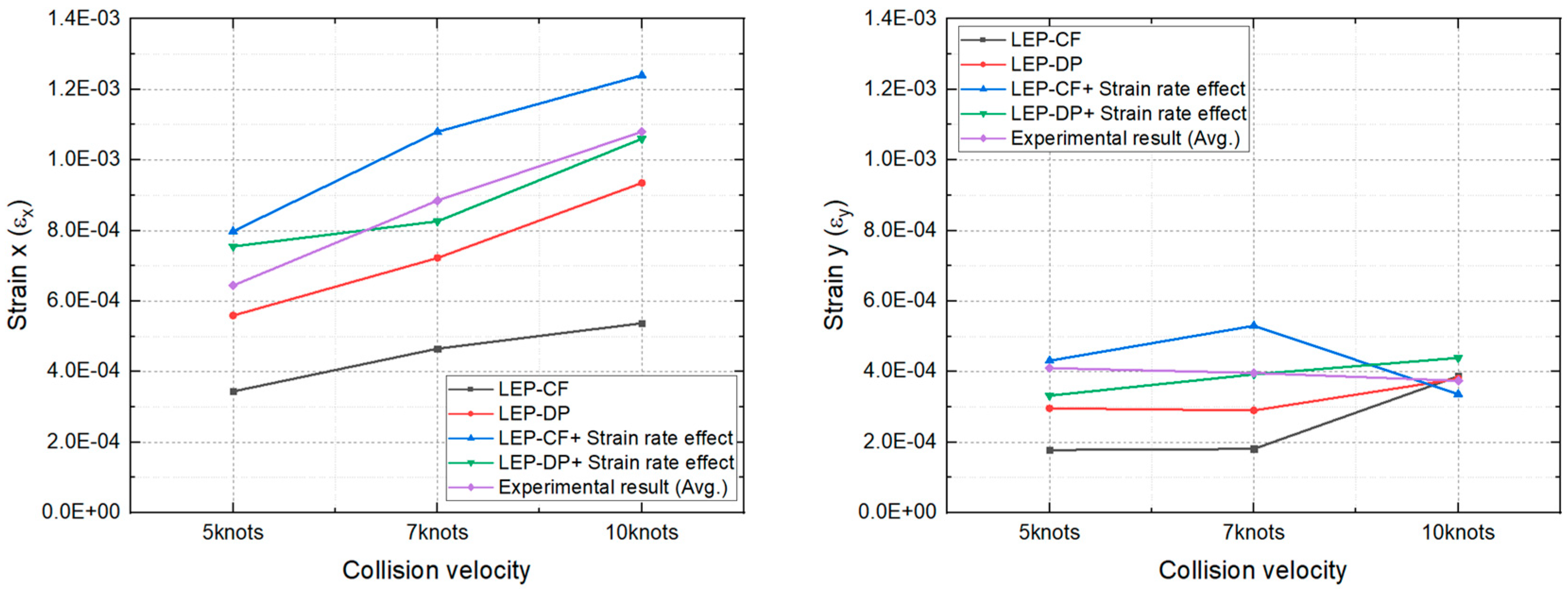
- Predicted strains on steel plate
- Ice collision force prediction results
4.5. Evaluation of Suitability for Each Combination of Ice Material Models
5. Conclusions
Author Contributions
Funding
Institutional Review Board Statement
Informed Consent Statement
Data Availability Statement
Acknowledgments
Conflicts of Interest
References
- Tangborn, A.; Kan, S.; Tangborn, W. Calculation of the Size of the Iceberg Struck by the Oil tanker Overseas Ohio. In Proceedings of the 14th IAHR Symposium on Ice, Potsdam, NY, USA, 27–31 July 1998; Volume 1, pp. 237–241. [Google Scholar]
- Gagnon, R. Results of numerical simulations of growler impact tests. Cold Reg. Sci. Technol. 2007, 49, 206–214. [Google Scholar] [CrossRef]
- Gagnon, R. A numerical model of ice crushing using a foam analogue. Cold Reg. Sci. Technol. 2011, 65, 335–350. [Google Scholar] [CrossRef]
- Kim, H.; Daley, C.; Colbourne, B. A numerical model for ice crushing on concave surfaces. Ocean Eng. 2015, 106, 289–297. [Google Scholar] [CrossRef]
- Kajaste-Rudnitski, J.; Kujala, P. Ship propagation through ice field. J. Struct. Mech. 2014, 47, 34–49. [Google Scholar]
- Song, M.; Kim, E.; Amdahl, J. Fluid-structure-interaction analysis of an ice block-structure collision. In Proceedings of the 23rd International Conference on Port and Ocean Engineering under Arctic Conditions, Trondheim, Norway, 14–18 June 2015. [Google Scholar]
- Zhu, L.; Qiu, X.; Chen, M.; Yu, T. Simplified ship-ice collision numerical simulations. In Proceedings of the ISOPE International Ocean and Polar Engineering Conference, Rhodes, Greece, 26 June–1 July 2016; pp. 1192–2016. [Google Scholar]
- Cai, W.; Zhu, L.; Yu, T.; Li, Y. Numerical simulations for plates under ice impact based on a concrete constitutive ice model. Int. J. Impact Eng. 2020, 143, 103594. [Google Scholar] [CrossRef]
- Han, D.; Lee, H.; Choung, J.; Kim, H.; Daley, C. Cone ice crushing tests and simulations associated with various yield and fracture criteria. Ships Offshore Struct. 2017, 12 (Suppl. S1), S88–S99. [Google Scholar] [CrossRef]
- Gutfraind, R.; Savage, S.B. Smoothed particle hydrodynamics for the simulation of broken-ice fields: Mohr–Coulomb-type rheology and frictional boundary conditions. J. Comput. Phys. 1997, 134, 203–215. [Google Scholar] [CrossRef]
- Zhang, N.; Zheng, X.; Ma, Q. Updated smoothed particle hydrodynamics for simulating bending and compression failure progress of ice. Water 2017, 9, 882. [Google Scholar] [CrossRef]
- Tuhkuri, J.; Polojärvi, A. A review of discrete element simulation of ice–structure interaction. Philos. Trans. R. Soc. A Math. Phys. Eng. Sci. 2018, 376, 20170335. [Google Scholar] [CrossRef]
- Tsarau, A.; Lubbad, R.; Løset, S. A numerical model for simulation of the hydrodynamic interactions between a marine floater and fragmented sea ice. Cold Reg. Sci. Technol. 2014, 103, 1–14. [Google Scholar] [CrossRef]
- Ji, S.; Li, Z.; Li, C.; Shang, J. Discrete element modeling of ice loads on ship hulls in broken ice fields. Acta Oceanol. Sin. 2013, 32, 50–58. [Google Scholar] [CrossRef]
- Jang, H.-S.; Hwang, S.-Y.; Lee, J.H. Experimental Evaluation and Validation of Pressure Distributions in Ice–Structure Collisions Using a Pendulum Apparatus. J. Mar. Sci. Eng. 2023, 11, 1761. [Google Scholar] [CrossRef]
- Barrette, P.D.; Jordaan, I.J. Pressure–temperature effects on the compressive behavior of laboratory-grown and iceberg ice. Cold Reg. Sci. Technol. 2003, 36, 25–36. [Google Scholar] [CrossRef]
- Jones, S.J. High strain-rate compression tests on ice. J. Phys. Chem. B 1997, 101, 6099–6101. [Google Scholar] [CrossRef]
- Petrovic, J. Review mechanical properties of ice and snow. J. Mater. Sci. 2003, 38, 1–6. [Google Scholar] [CrossRef]
- Zhang, W.; Li, J.; Li, L.; Yang, Q. A systematic literature survey of the yield or failure criteria used for ice material. Ocean Eng. 2022, 254, 111360. [Google Scholar] [CrossRef]
- Kim, J.-H.; Kim, Y.; Kim, H.-S.; Jeong, S.-Y. Numerical simulation of ice impacts on ship hulls in broken ice fields. Ocean Eng. 2019, 182, 211–221. [Google Scholar] [CrossRef]
- Jeon, S.; Kim, Y. Numerical simulation of level ice–structure interaction using damage-based erosion model. Ocean Eng. 2021, 220, 108485. [Google Scholar] [CrossRef]
- Gagnon, R. Analysis of data from bergy bit impacts using a novel hull-mounted external Impact Panel. Cold Reg. Sci. Technol. 2008, 52, 50–66. [Google Scholar] [CrossRef]
- Liu, Z.; Amdahl, J.; Løset, S. Plasticity based material modelling of ice and its application to ship–iceberg impacts. Cold Reg. Sci. Technol. 2011, 65, 326–334. [Google Scholar] [CrossRef]
- Zhang, J.; Liu, Z.; Ong, M.C.; Tang, W. Numerical simulations of the sliding impact between an ice floe and a ship hull structure in ABAQUS. Eng. Struct. 2022, 273, 115057. [Google Scholar] [CrossRef]
- Islam, M.; Mills, J.; Gash, R.; Pearson, W. A literature survey of broken ice-structure interaction modelling methods for ships and offshore platforms. Ocean Eng. 2021, 221, 108527. [Google Scholar] [CrossRef]
- Carney, K.S.; Benson, D.J.; DuBois, P.; Lee, R. A phenomenological high strain rate model with failure for ice. Int. J. Solids Struct. 2006, 43, 7820–7839. [Google Scholar] [CrossRef]
- Shi, C.; Hu, Z.; Ringsberg, J.; Luo, Y. Validation of a temperature-gradient-dependent elastic-plastic material model of ice with finite element simulations. Cold Reg. Sci. Technol. 2017, 133, 15–25. [Google Scholar] [CrossRef]
- Zhu, L.; Cai, W.; Chen, M.; Tian, Y.; Bi, L. Experimental and numerical analyses of elastic-plastic responses of ship plates under ice floe impacts. Ocean Eng. 2020, 218, 108174. [Google Scholar] [CrossRef]
- Sain, T.; Narasimhan, R. Constitutive modeling of ice in the high strain rate regime. Int. J. Solids Struct. 2011, 48, 817–827. [Google Scholar] [CrossRef]
- Bhat, S.; Choi, S.; Wierzbicki, T.; Karr, D. Failure Analysis of Impacting Ice Floes. In Proceedings of the 8th International OMAE Conference, The Hague, The Netherlands, 19–23 March 1989; pp. 275–285. [Google Scholar]
- Pernas-Sánchez, J.; Pedroche, D.; Varas, D.; López-Puente, J.; Zaera, R. Numerical modeling of ice behavior under high velocity impacts. Int. J. Solids Struct. 2012, 49, 1919–1927. [Google Scholar] [CrossRef]
- Mokhtari, M.; Kim, E.; Amdahl, J. Pressure-dependent plasticity models with convex yield loci for explicit ice crushing simulations. Mar. Struct. 2022, 84, 103233. [Google Scholar] [CrossRef]
- Tippmann, J.D. Development of a Strain Rate Sensitive Ice Material Model for Hail Ice Impact Simulation; University of California: San Diego, CA, USA, 2011. [Google Scholar]
- Gagnon, R.; Derradji-Aouat, A. First results of numerical simulations of bergy bit collisions with the CCGS terry fox icebreaker. In Proceedings of the 18th IAHR International Symposium on Ice, Sapporo, IAHR & AIRH, Sapporo, Japan, 28 August–1 September 2006. [Google Scholar]
- Gao, Y.; Hu, Z.; Wang, J. Sensitivity analysis for iceberg geometry shape in ship-iceberg collision in view of different material models. Math. Probl. Eng. 2014, 2014, 414362. [Google Scholar] [CrossRef]
- Obisesan, A.; Sriramula, S. Efficient response modelling for performance characterisation and risk assessment of ship-iceberg collisions. Appl. Ocean Res. 2018, 74, 127–141. [Google Scholar] [CrossRef]
- Hallquist, J.O. LS-DYNA Theory Manual; Livermore Software Technology Corporation: Livermore, CA, USA, 2006; pp. 19.196–19.197. [Google Scholar]
- SIMULIA, ABAQUS/Standard User’s Manual, Version 6.14; Dassault Systèmes Simulia Corp.: Johnston, RI, USA, 2014.
- Tippmann, J.D.; Kim, H.; Rhymer, J.D. Experimentally validated strain rate dependent material model for spherical ice impact simulation. Int. J. Imp. Eng. 2013, 57, 43–54. [Google Scholar] [CrossRef]
- Keune, J. Development of a Hail Ice Impact Model and the Dynamic Compressive Strength Properties of Ice. Ph.D. Thesis, Purdue University, West Lafayette, IN, USA, 2004. [Google Scholar]


| Material Behavior | Model | Reference |
|---|---|---|
| Yield criteria | Crushable Foam | Gagnon [3], Kim, et al. [4], Liu et al. [23] |
| Drucker–Prager | Kajaste-Rudnitski & Kujala [5] | |
| Damage model | Ductile Damage | Han, et al. [9], Kim, et al. [20], Jeon & Kim [21] |
| Strain rate effect | Tippmann [33] |
| Models | Constitutive Equation | Yield Criteria |
|---|---|---|
| LEPP-CF | Linear elastic-perfectly plastic | Crushable Foam |
| LEPP-DP | Linear elastic-perfectly plastic | Drucker–Prager |
| LEP-CF | Linear elastic-plastic | Crushable Foam |
| LEP-DP | Linear elastic-plastic | Drucker–Prager |
| LEPP | Crushable Foam (CF) (Obisesan and Sriramula [36]) | Drucker–Prager (DP) (Jeon and Kim [21]) | |||
|---|---|---|---|---|---|
| Parameter | Compression Yield Stress Ratio | Hydrostatic Yield Stress Ratio | Friction Angle | Flow Stress Ratio | Dilation Angle |
| Value | 1.49 | 1.79 | 36 deg | 1 | 12 deg |
| LEP | Crushable Foam (CF) | Drucker–Prager (DP) | ||
|---|---|---|---|---|
| Hardening Value | Stress | Strain | Stress | Strain |
| 0.5 MPa | 0 | 0.5 MPa | 0 | |
| 3.3 MPa | 0.019 | 3 MPa | 0.025 | |
| 3.3 MPa | 0.5 | 3 MPa | 0.5 | |
| FEA Result | LEPP-CF | LEPP-DP | LEP-CF | LEPP-DP |
|---|---|---|---|---|
| Peak force [kN] | 28.2 | 27.9 | 27.8 | 28.2 |
| Displacement [mm] | 5.02 | 5.1 | 4.98 | 4.92 |
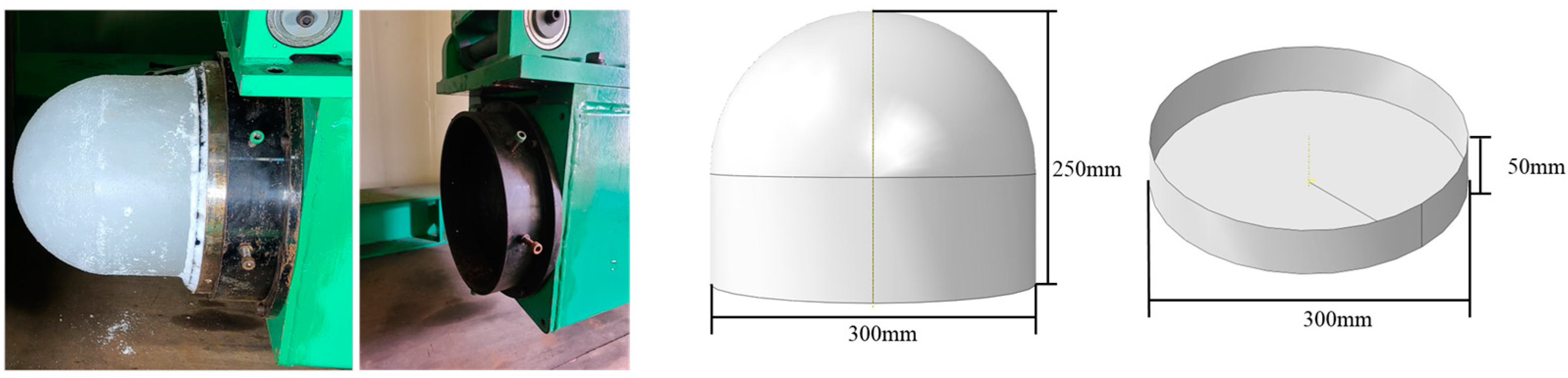
| Ice Specimen | Ice Holder | Steel Plate | Steel Jig | |
|---|---|---|---|---|
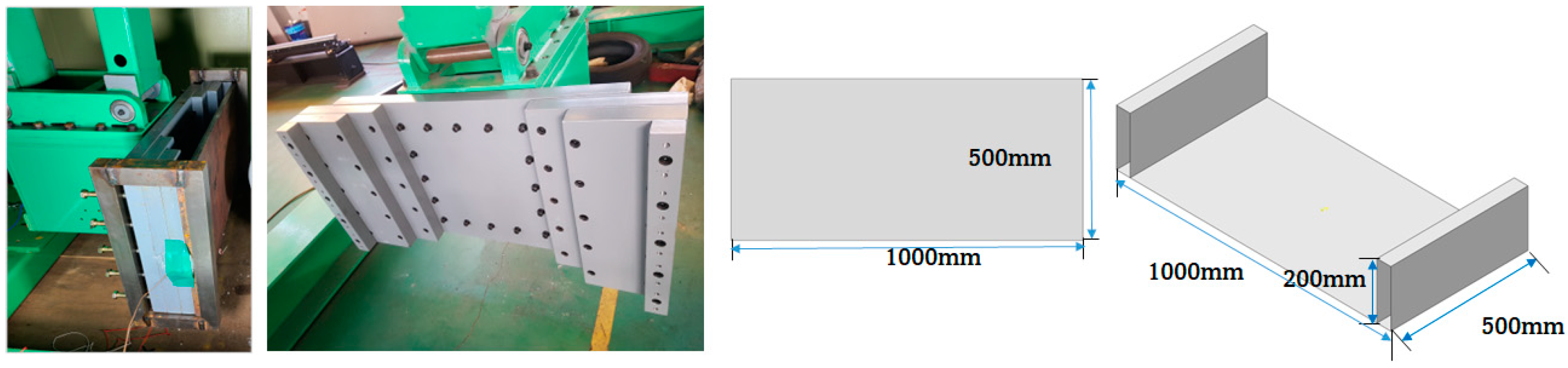
| Geometry | = 300 mm (Figure 10) | = 300 mm (Figure 10) | 1000 × 500 × 20 mm (Figure 11) | 200 × 50 × 500 mm (Figure 11) |
| Finite element | Shell Element (S4R) | Rigid Element (R3D4) | Solid Element (C3D8R) | Rigid Element (R3D4) |
| Contact | Hard contact with steel plate (penalty contact, frictionless) | Tie condition with ice | Hard contact with ice (penalty contact, frictionless) | Tie condition with steel plate |
| Mesh Size | Max. Force [kN] | Normalized Force | CPU Time |
|---|---|---|---|
| 7 mm | 23.69 | 0.948 | 0 H 25 min |
| 5 mm | 24.41 | 0.976 | 1 H 15 min |
| 3 mm | 24.96 | 0.999 | 3 H 10 min |
| 2 to 5 mm | 24.99 | 1.000 | 2 H 05 min |
| Collision Velocity (Kts) | Experiment (Avg.) | LEPP-CF | LEPP-DP | LEP-CF | LEP-DP |
|---|---|---|---|---|---|
| 5 (2.57 m/s) | 6.44 | 3.77 (41.4%) | 3.59 (44.3%) | 3.44 (46.7%) | 5.59 (13.2%) |
| 7 (3.61 m/s) | 8.85 | 4.72 (46.6%) | 6.19 (30.1%) | 4.65 (47.4%) | 7.22 (18.4%) |
| 10 (5.13 m/s) | 1.08 | 5.26 (51.3%) | 5.87 (45.6%) | 5.37 (50.3%) | 9.35 (13.4%) |
| Difference | - | 46.5% | 40.0% | 48.1% | 15.0% |
| Collision Velocity (Kts) | Experiment (Avg.) | LEPP-CF | LEPP-DP | LEP-CF | LEP-DP |
|---|---|---|---|---|---|
| 5 (2.57 m/s) | 4.10 | 1.76 (57.1%) | 2.01 (50.9%) | 1.78 (56.5%) | 2.96 (27.9%) |
| 7 (3.61 m/s) | 3.96 | 2.58 (34.9%) | 2.51 (36.6%) | 1.81 (23.1%) | 2.90 (26.8%) |
| 10 (5.13 m/s) | 3.74 | 3.09 (17.3%) | 2.34 (37.4%) | 3.87 (3.4%) | 3.80 (1.5%) |
| Difference | - | 36.4% | 41.7% | 38.1% | 18.7% |
| Collision Velocity (Kts) | Experiment (Avg.) | LEPP-CF | LEPP-DP | LEP-CF | LEP-DP |
|---|---|---|---|---|---|
| 5 (2.57 m/s) | 32.4 | 16.7 (48.5%) | 20.1 (37.9%) | 19.3 (40.3%) | 27.5 (15.1%) |
| 7 (3.61 m/s) | 45.3 | 31.8 (29.8%) | 25.6 (43.5%) | 21.4 (52.8%) | 36.9 (18.5%) |
| 10 (5.13 m/s) | 70.4 | 24.99 (64.5%) | 36.6 (48.0%) | 23.9 (66.1%) | 52.8 (25.0%) |
| Difference | - | 47.6% | 43.1% | 53.1% | 19.6% |
| Collision Velocity (Knots) | Experiment (Avg.) | LEPP-CF | LEPP-DP | LEP-CF | LEP-DP |
|---|---|---|---|---|---|
| 5 (2.57 m/s) | 6.44 | 3.30 (48.8%) | 4.82 (25.2%) | 7.98 (23.9%) | 7.55 (17.3%) |
| 7 (3.61 m/s) | 8.85 | 4.72 (46.6%) | 1.07 (21.3%) | 1.08 (21.7%) | 8.26 (6.7%) |
| 10 (5.13 m/s) | 1.08 | 5.26 (51.3%) | 1.73 (29.6%) | 1.24 (14.5%) | 1.06 (2.0%) |
| Difference | - | 48.9% | 30.2% | 20.0% | 8.7% |
| Collision Velocity (Knots) | Experiment (Avg.) | LEPP-CF | LEPP-DP | LEP-CF | LEP-DP |
|---|---|---|---|---|---|
| 5 (2.57 m/s) | 4.10 × 10⁻⁴ | 1.83 (55.4%) | 1.95 (52.4%) | 4.31 (5.03%) | 3.32 (19.0%) |
| 7 (3.61 m/s) | 3.96 × 10⁻⁴ | 2.59 (34.6%) | 3.78 (4.6%) | 5.30 (33.9%) | 3.92 (0.9%) |
| 10 (5.13 m/s) | 3.74 × 10⁻⁴ | 3.09 (17.4%) | 4.67 (24.8%) | 3.36 (10.0%) | 4.39 (17.4%) |
| Difference | - | 35.8% | 27.3% | 16.3% | 12.4% |
| Collision Velocity (Knots) | Experiment (Avg.) | LEPP-CF | LEPP-DP | LEP-CF | LEP-DP |
|---|---|---|---|---|---|
| 5 (2.57 m/s) | 32.4 | 17.8 (45.1%) | 23.2 (28.4%) | 47.6 (46.9%) | 36.5 (12.7%) |
| 7 (3.61 m/s) | 45.3 | 28.7 (36.6%) | 56.1 (23.8%) | 49.9 (10.2%) | 39.9 (11.9%) |
| 10 (5.13 m/s) | 70.4 | 31.8 (54.8%) | 78.2 (11.1%) | 61.5 (12.6%) | 61.8 (12.2%) |
| Difference | - | 45.5% | 21.1% | 23.2% | 12.3% |
| Collision Velocity (Knots) | LEP-CF | LEP-DP | LEP-CF + Strain Rate Effect | LEP-DP + Strain Rate Effect |
|---|---|---|---|---|
| 5 (2.57 m/s) | 3.44 (46.7%) | 5.59 (13.2%) | 7.98 (23.9%) | 7.55 (17.3%) |
| 7 (3.61 m/s) | 4.65 (47.4%) | 7.22 (18.4%) | 1.08 (21.7%) | 8.26 (6.7%) |
| 10 (5.13 m/s) | 5.37 (50.3%) | 9.35 (13.4%) | 1.24 (14.5%) | 1.06 (2.0%) |
| Avg. Difference | 48.1% | 15.0% | 20.0% | 8.7% |
| Collision Velocity (Knots) | LEP-CF | LEP-DP | LEP-CF + Strain Rate Effect | LEP-DP + Strain Rate Effect |
|---|---|---|---|---|
| 5 (2.57 m/s) | 1.78 (56.5%) | 2.96 (27.9%) | 4.31 (5.03%) | 3.32 (19.0%) |
| 7 (3.61 m/s) | 1.81 (23.1%) | 2.90 (26.8%) | 5.30 (33.9%) | 3.92 (0.9%) |
| 10 (5.13 m/s) | 3.87 (3.4%) | 3.80 (1.5%) | 3.36 (10.0%) | 4.39 (17.4%) |
| Avg. Difference | 38.1% | 18.7% | 16.3% | 12.4% |
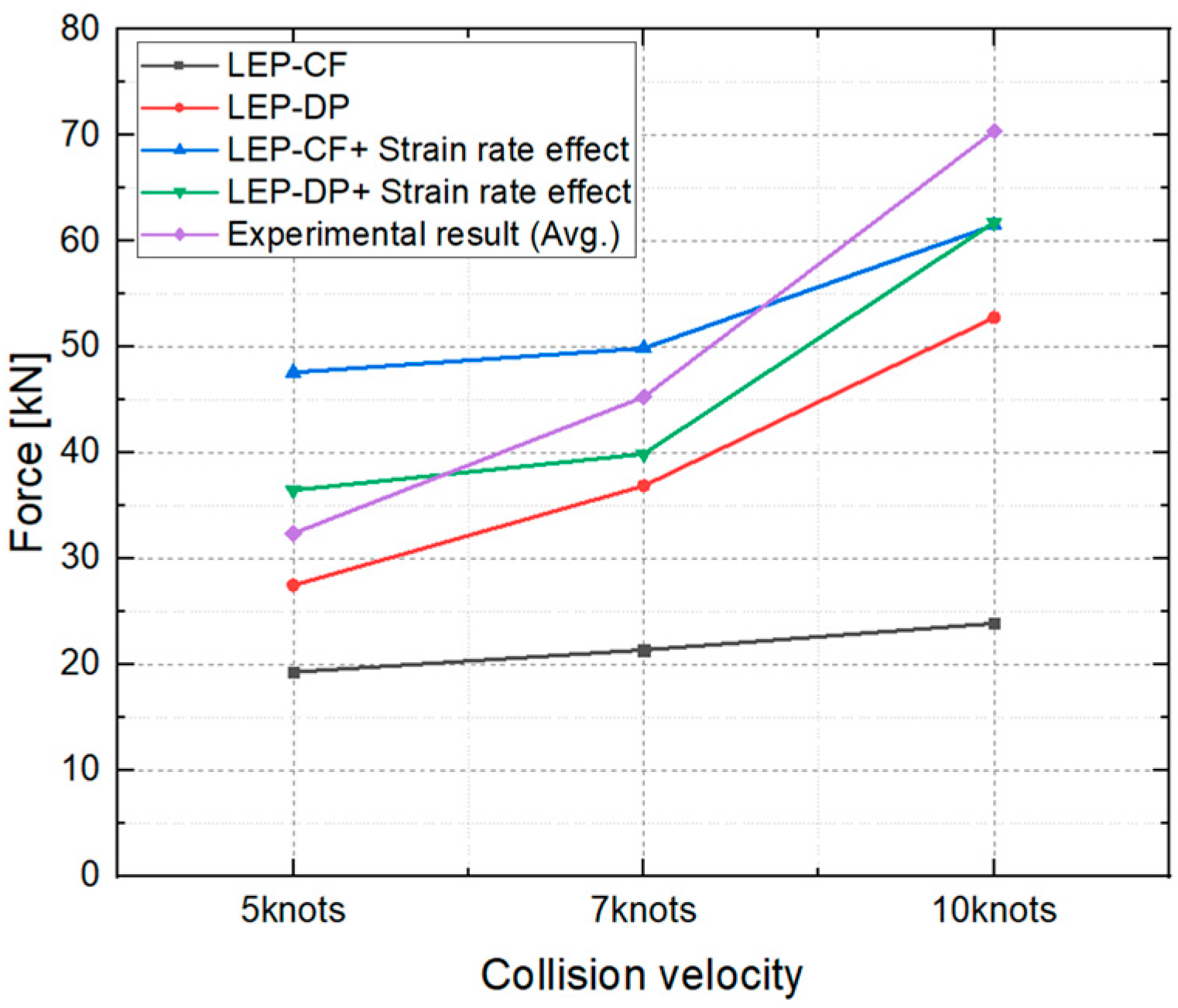
| Collision Velocity (Knots) | LEP-CF | LEP-DP | LEP-CF + Strain Rate Effect | LEP-DP + Strain Rate Effect |
|---|---|---|---|---|
| 5 (2.57 m/s) | 19.3 (40.3%) | 27.5 (15.1%) | 47.6 (−46.9%) | 36.5 (−12.7%) |
| 7 (3.61 m/s) | 21.4 (52.8%) | 36.9 (18.5%) | 49.9 (−10.2%) | 39.9 (11.9%) |
| 10 (5.13 m/s) | 23.9 (66.1%) | 52.8 (25.0%) | 61.5 (12.6%) | 61.8 (12.2%) |
| Avg. Difference | 53.1% | 19.6% | 23.2% | 12.3% |
| FEA Result | Material Model | 5 kts (2.57 m/s) | 7 kts (3.61 m/s) | 10 kts (5.13 m/s) | Mean Diff. |
|---|---|---|---|---|---|
| Max. strain x () (Difference with experiment) | LEP-DP | 5.59 × 10⁻⁴ (13.2%) | 7.22 × 10⁻⁴ (18.4%) | 8.26 × 10⁻⁴ (13.4%) | 15.0% |
| LEP-DP + Strain rate effect | 7.55 × 10⁻⁴ (17.3%) | 8.26 × 10⁻⁴ (6.7%) | 1.06 × 10⁻³ (2.0%) | 8.7% | |
| Max. strain y () (Difference with experiment) | LEP-DP | 2.96 × 10⁻⁴ (27.9%) | 2.90 × 10⁻⁴ (26.8%) | 3.80 × 10⁻⁴ (1.5%) | 17.7% |
| LEP-DP + Strain rate effect | 3.32 × 10⁻⁴ (19.0%) | 3.92 × 10⁻⁴ (0.9%) | 4.39 × 10⁻⁴ (17.4%) | 12.4% | |
| Max. force (Difference with experiment) | LEP-DP | 27.5 (15.1%) | 36.9 (18.5%) | 52.8 (25.0%) | 19.6% |
| LEP-DP + Strain rate effect | 36.5 (12.7%) | 39.9 (11.9%) | 61.8 (12.2%) | 12.3% |
Disclaimer/Publisher’s Note: The statements, opinions and data contained in all publications are solely those of the individual author(s) and contributor(s) and not of MDPI and/or the editor(s). MDPI and/or the editor(s) disclaim responsibility for any injury to people or property resulting from any ideas, methods, instructions or products referred to in the content. |
© 2024 by the authors. Licensee MDPI, Basel, Switzerland. This article is an open access article distributed under the terms and conditions of the Creative Commons Attribution (CC BY) license (https://creativecommons.org/licenses/by/4.0/).
Share and Cite
Jang, H.-S.; Hwang, S.; Yoon, J.; Lee, J.H. Numerical Analysis of Ice–Structure Impact: Validating Material Models and Yield Criteria for Prediction of Impact Pressure. J. Mar. Sci. Eng. 2024, 12, 229. https://doi.org/10.3390/jmse12020229
Jang H-S, Hwang S, Yoon J, Lee JH. Numerical Analysis of Ice–Structure Impact: Validating Material Models and Yield Criteria for Prediction of Impact Pressure. Journal of Marine Science and Engineering. 2024; 12(2):229. https://doi.org/10.3390/jmse12020229
Chicago/Turabian StyleJang, Ho-Sang, Seyun Hwang, Jaedeok Yoon, and Jang Hyun Lee. 2024. "Numerical Analysis of Ice–Structure Impact: Validating Material Models and Yield Criteria for Prediction of Impact Pressure" Journal of Marine Science and Engineering 12, no. 2: 229. https://doi.org/10.3390/jmse12020229