Maximizing Efficiency in the Suez Canal: A New Approach to Evaluate the Impact of Optimal Time-Varying Tolls on Ship Arrival Times

Abstract

In the existing literature, an optimal time-varying toll scheme has been proposed for the Suez Canal to address the inefficiency of numerous ships queuing and waiting at the anchorage area to enter the canal. The primary objective of this tolling strategy is to alleviate the significant issue of ships queuing at the canal’s anchorage area. This stands in contrast to the current tolling system employed by the Suez Canal, which primarily aims to recover the management and operational costs associated with ship passage through the canal. However, the existing literature has yet to explore how the arrival times of ships at the anchorage area will change after implementing the optimal time-varying toll scheme. The goal is to ensure that the equilibrium cost of each tolled ship does not result in losses and achieve maximum efficiency in eliminating queueing at the anchorage area. To address this gap, this paper adopts the principle of cost equilibrium conservation and utilizes the Point-Slope Form to derive two mathematical formulas representing all ships’ post-toll arrival times at the anchorage area of the Suez Canal. These formulas are specifically derived for two categories of tolled ships: those that enter the canal earlier than the latest entry time regulated by the canal authorities and those that enter later. The derived formulas are concise and comparative, strengthening the theoretical underpinnings of the current pricing model for a queuing canal. Furthermore, they serve as valuable references for canal authorities in devising pertinent measures, such as organizing the scheduling of canal pilots, to facilitate the implementation of the optimal time-varying toll scheme.

1. Introduction

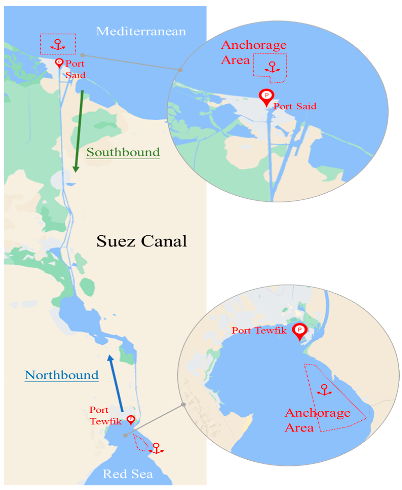
Prior to the expansion of the Suez Canal, the canal’s narrow passage restricted the passage of large ships, particularly those with oversized hulls. However, since the completion of the canal expansion in 2016, a majority of these large ships can now navigate through the canal, excepting ULCC super tankers. While the expansion increased the canal’s overall capacity, the inclusion of previously inaccessible large ships has led to a congestion issue, resulting in a notable queuing problem in the anchorage area. To address the persistent challenge of extensive ship queues at the entrance (the anchorage area) of the Suez Canal (please refer to Figure 1 for the location of the anchorage areas, southbound and northbound routes), one potential solution for canal authorities is to consider implementing queuing pricing measures. This pricing strategy aims to encourage a more dispersed arrival pattern of ships in the anchorage area. Such an approach holds the potential to alleviate inefficiencies caused by prolonged ship queues and presents an effective resolution to the problem.

In the existing literature on queuing pricing for the Suez Canal, Laih et al. [2] were pioneers in developing an optimal time-varying toll scheme. Their primary goal was to eliminate the cumulative queuing time for all ships in the canal’s anchorage area, aiming for the most efficient utilization of the canal. Subsequently, Sun and Laih [3] delved deeper into the effects of the optimal time-varying toll scheme on ship arrivals at the anchorage area. Specifically, their study investigated how each ship could sequentially adjust its arrival time after the implementation of this toll scheme, with the aim of establishing a scenario where no queuing occurs for entry into the canal. This study assumed that the intervals between ship arrivals at the canal anchorage area follow a uniform distribution. Starting from the initiation of queuing, these intervals progressively accumulate until the termination of queuing. Based on this assumption, each ship’s pre-toll and post-toll arrival times at the anchorage area can be calculated. Consequently, by comparing the post-toll arrival time with the pre-toll arrival time, the postponement in arrival time at the anchorage area for each tolled ship can be determined.

The work by Sun and Laih [3], as mentioned above, offers practical advantages for both ship owners and canal authorities by facilitating the convenient scheduling of each queued ship’s entry into the canal. However, the methodology of this study has two debatable aspects. Firstly, the assumption that the intervals between ship arrivals at the anchorage area follow a uniform distribution lacks sufficient supporting statistical data to validate its generality. Consequently, the justification for this assumption appears somewhat weak. Secondly, the approach of calculating each ship’s arrival time at the anchorage area, starting from the initiation of the queueing process and accumulating the same arrival interval until the queueing is terminated, poses challenges. This method becomes problematic as the error in the accumulated calculation magnifies with an increasing number of ships, making it difficult to satisfy the condition where the schedule delay cost (the penalty costs for either early or late entry into the canal) is absolutely the same before and after the toll implementation. In other words, the necessary condition of maintaining the same equilibrium cost, regardless of toll implementation, cannot be met. Consequently, their methodology deviates from the principle of cost equilibrium conservation for all ships, leading to discrepancies between the calculated arrival times of tolled ships at the anchorage area and the authentic results under an equilibrium state. As a result, its practical value as a reference is diminished.

To address the aforementioned controversies and enhance both the theoretical basis and practical significance of the optimal time-varying toll scheme for a queuing canal, this paper seeks to derive mathematical formulas based on the principle of cost equilibrium conservation. This principle dictates that all ships maintain the same schedule delay costs before and after toll implementation. The derived formulas in this paper represent the arrival times at the anchorage area for two categories of tolled ships: those arriving early (including on time) and the remaining ships arriving late. These formulas are concise and offer a comparative framework. The derivation of these formulas reinforces the theoretical foundation of the pricing model for a queuing canal. Moreover, it provides valuable references for canal authorities in planning and allocating associated supporting measures, such as organizing the scheduling of canal pilots, when considering the implementation of the optimal time-varying toll scheme.

The primary academic contribution of this paper lies in deriving mathematical formulas for the arrival times of all tolled ships at the Suez Canal’s anchorage area using the Point-Slope Form. These formulas are developed on the basis that the cost associated with early or late entry into the canal remains consistent for each ship, both before and after implementing the optimal time-varying toll scheme. By ensuring equal schedule delay costs for each ship, regardless of toll implementation, these derived formulas not only meet the requirement of maintaining cost equilibrium for all ships before and after toll implementation, but also contribute to achieving maximum efficiency in eliminating queuing in the canal’s anchorage area. The methodologies and findings presented in this paper fill a gap in the existing literature by overcoming the limitations associated with assuming a uniform distribution for the intervals between ship arrivals at the canal’s anchorage area, as proposed by Sun and Laih [3]. Simultaneously, the derived formulas make it possible to guarantee the principle of cost equilibrium conservation for each ship before and after toll implementation.

The paper is structured as follows: In Section 2, we provide a comprehensive review of the queuing pricing models relevant to this study, including various tolling structures and user behavior after toll implementation. Section 3 conducts a retrospective analysis of equilibrium cost calculations for ships queuing at the canal’s anchorage area and the derivation of the optimal time-varying toll scheme designed to facilitate queue-free entry into the canal. In Section 4, we employ the Point-Slope Form to derive two mathematical formulas for ships with time-early and time-late schedules. These formulas determine the arrival times of all tolled ships at the canal’s anchorage area and are specifically crafted to ensure the principle of cost equilibrium conservation. This principle dictates that each ship maintains the same equilibrium cost before and after toll implementation. In Section 5, we conduct a numerical analysis based on the latest official statistical data from the Suez Canal. This analysis focuses on the results obtained in Section 4, providing valuable insights and guidance for canal authorities. Finally, Section 6 presents the conclusion and offers recommendations based on the findings of this study.

2. Literature Review

Vickrey [4] pioneered the development of a queuing pricing model specifically tailored for a road bottleneck. His model aimed to establish an optimal variable toll scheme to effectively eliminate the waiting time experienced by commuters queuing at the entry of a road bottleneck. Subsequently, numerous scholars have expanded upon Vickrey’s groundwork to address queuing phenomena and propose pricing strategies for bottleneck users. For instance, Small [5] assessed the time cost of queuing for commuters in the San Francisco Bay Area, incorporating considerations of penalty cost incurred by commuters for arriving at their workplaces either early or late due to queuing. Cohen [6] applied Vickrey’s model to analyze the welfare impact on different income groups after the implementation of optimal variable tolls. Additionally, Braid [7], Arnott et al. [8], and Laih [9] further utilized Vickrey’s bottleneck model to devise optimal time-varying tolls (also known as optimal fine tolls) and other toll schemes aimed at eliminating or reducing queuing time for commuters approaching a road bottleneck. Tabuchi [10] broadened the scope by considering the coexistence of road bottlenecks and mass transit railways. He compared the welfare implications of railway fares to those of road pricings (e.g., optimal uniform toll, optimal variable toll, etc.) for commuters. Small [11] commented on the background assumptions of the queuing pricing model, suggesting that incorporating factors such as the presence of heterogeneous commuters or multiple bottleneck areas would enhance the practical value of the derived results, aligning them more closely with real-world situations. Bao et al. [12] contributed to the field by developing a public holiday traffic congestion model and evaluated the impact of an optimal time-varying toll scheme, compared to a free toll policy, on social welfare.

The optimal time-varying toll scheme that we have mentioned above holds the potential to effectively eliminate the inefficient queuing phenomenon for bottleneck users. However, one drawback of implementing this scheme lies in the complexity associated with continuously changing toll amounts. To address this challenge, an alternative approach involves considering a simpler tolling structure, such as a step toll scheme. Laih [9] was the first to propose a step toll scheme explicitly designed for a commuting road bottleneck. This tolling structure is seamlessly integrated into the optimal time-varying toll scheme framework. An optimal n-step toll scheme, where n represents the number of steps, could reduce n/(n + 1) of the total queuing time for all commuters.

In addition to the aforementioned studies on Laih’s step toll, Lindsey et al. [13] proposed an improved version of the third Breaking model after comparing it with the most representative ADL model (constructed by Arnott et al. [8]) and the Laih model (constructed by Laih [9]). Their proposed step toll scheme is constructed based on the inevitable behavior of commuter vehicles slowing down or stopping in the queuing pricing theory. Its toll structure is slightly different from other step toll models, providing relevant scholars with material for subsequent evaluation and comparison.

Because the above-mentioned step toll scheme only explores the decision behavior of homogeneous commuters (road users) after toll implementation, to overcome this limitation, Xiao et al. [14] introduced heterogeneous commuters into the road bottleneck queuing pricing model. They formulated the optimal coarse toll scheme (similar to a single-step toll scheme) and investigated the departure patterns of commuters after the implementation of this toll scheme. This study also demonstrated that implementing the optimal coarse toll scheme is consistent with the Pareto optimum.

Furthermore, Vincent and van den Berg [15] investigated the welfare distribution effects among heterogeneous commuters after the implementation of a single-step toll scheme. This study analyzed and compared three queuing pricing models: the ADL model, the Laih model, and the Breaking model. In the Laih model, the single-step toll amount for heterogeneous commuters fell between the equilibrium cost and the optimal time-varying tolls. Furthermore, the welfare distribution effects after toll implementation in the Laih model were straightforward and clear. In contrast, the other two models did not exhibit such simplicity in determining the single-step toll amount for heterogeneous commuters, and the welfare distribution effects after toll implementation were more complex. Specifically, the welfare distribution effects of the Breaking model after the implementation of a single-step toll scheme were most detrimental to commuters with lower time value and those who could not afford to be late.

Moreover, Li et al. [16] constructed an optimal step toll scheme by considering the premise that the utility of activities at home and the workplace for heterogeneous commuters varies significantly over time. The study found that the queuing elimination effect of the step toll scheme derived from the linear marginal utility model surpassed that of the traditional step toll scheme derived from the fixed marginal utility model. However, neglecting the heterogeneity of commuters would underestimate the queuing elimination effect of the optimal step toll scheme.

In addition to road bottlenecks, the queuing pricing model has also been applied in maritime transportation. The notable application is for ships queuing in the anchorage area to enter a canal. Laih et al. [2] were the first to develop an optimal time-varying toll scheme for ships queuing to enter the Suez Canal. The primary objective of this toll scheme is to eliminate queuing at the anchorage area and enhance the efficiency of canal utilization. Subsequently, Sun and Laih [3] conducted a study that examined the time intervals between ship arrivals at the anchorage area of the Suez Canal before and after implementing the optimal time-varying toll scheme. Their analysis provided insights into the differences in arrival times at the anchorage area for all ships before and after the toll implementation, shedding light on the impact of the toll scheme on arrival patterns.

Du et al. [17] assessed the impact of the Suez Canal traffic control system and the stepwise toll pricing policy on the optimal navigation schedule for regularly scheduled container ships. This paper develops a mixed-integer nonlinear programming model and examines the optimal navigation schedule through a case study of 13,000 TEU container ship with long-haul voyage passing through the Suez Canal. Although the stepwise toll pricing in this paper is not directly related to the queuing pricing implemented in the canal anchorage area, canal authorities must consider the interconnected effects and outcomes on the reduction of canal operating costs and efficiency improvement when implementing both the stepwise toll pricing for passing through the canal and the queuing pricing for ships waiting in the canal’s anchorage.

Similar to the canal queuing pricing, Wang and Li [18] conducted a study addressing congestion issues for ships navigating through a channel with a lock. They developed a queuing pricing model that focuses on dynamic fee structures, using container ships as a case study. The model transforms the costs incurred by ships queuing and docking at a lock into congestion fees collected by the authorities. The primary goal is to eliminate the queuing time for container ships at a lock, thereby effectively reducing social and economic losses and improving the overall efficiency of lock services. Moreover, this study delves into the decision-making process of departure times for container ships within the timeframe of the dynamic fee structure at a lock to maximize utility. Finally, the paper uses numerical analysis, taking the example of the Three Gorges Dam on the Yangtze River, to demonstrate the applicability of their queuing pricing model.

In conclusion, Li et al. [19] conducted a thorough literature review and classification of works related to bottleneck models, spanning various research contexts including roads, canals, and ports. Their study utilized bibliometric analysis and examined a total of 232 papers published over 50 years. This review yielded valuable insights into the evolution of bottleneck models over the past half-century, illuminating the current state of the field and offering predictions regarding potential future developments and prospects.

3. A Retrospection of the Optimal Time-Varying Toll Scheme for the Suez Canal

Building upon relevant studies, such as Laih et al. [2] and Sun and Laih [3], regarding queuing pricing in the canal’s anchorage area, as discussed in Section 2, and considering the current operational status of the Suez Canal, we summarize the underlying assumptions of the queuing pricing model for the Suez Canal as follows: Firstly, all ships must queue and wait to enter the canal, and the queueing occurs exclusively at the anchorage area of the canal. Secondly, all queued ships are served in the order of their arrival, adhering to a first-come, first-served basis, and it is mandatory for them to enter the canal prior to 11:00 PM. Thirdly, each ship independently determines its arrival time at the anchorage area of the canal, thereby making the cost for each ship dependent on its specific arrival time. Fourthly, the cost function assigned to each ship encompasses not only the cost incurred during waiting in the queue, but also accounts for the potential costs associated with entering the canal either early or late due to queuing. Please note that the current navigation toll imposed on ships passing through the canal is unrelated to the queuing process and is not included in this cost function. Based on the above scenarios, the potential time schedules for all ships arriving at the anchorage area of the Suez Canal and queuing for entry can be represented as follows:

$$T_E\left(t\right)=t^{*}-\left(t+T_Q\left(t\right)\right), for t+T_Q\left(t\right)<t^{*} or t<\tilde{t}$$

(1)

$$\tilde{t}+T_Q\left(\tilde{t}\right)=t^{*}$$

(2)

$$T_L\left(t\right)=\left(t+T_Q\left(t\right)\right)-t^{*}, for t+T_Q\left(t\right)>t^{*} or t>\tilde{t}$$

(3)

In Equations (1)–(3), $t$ denotes the arrival time of the ship at the anchorage area, signifying when the ship arrives at the Suez Canal’s anchorage area and completes the check-in procedure. $T_Q\left(t\right)$ represents the waiting time duration for each arriving ship in the queue before entering the canal. To align with the canal authorities’ requirement for all ships to enter the canal before 23:00, we designate the schedule where a ship enters the canal precisely at $t^{*}$ (=23:00) as an on-time schedule, depicted by Equation (2). This implies that when the arrival time of a ship at the anchorage area is $\tilde{t}$, the ship can enter the canal on time at $t^{*}$ after waiting in the queue. Furthermore, schedules in which ships enter the canal before $t^{*}$ and after $t^{*}$ are defined as time-early and time-late schedules, respectively, as indicated in Equations (1) and (3). The arrival times at the anchorage for these ships are earlier and later than $\tilde{t}$, and they enter the canal earlier and later than $t^{*}$ after waiting in the queue. $T_E\left(t\right)$ and $T_L\left(t\right)$ represent the durations by which these ships enter the canal earlier and later, respectively.

Building upon the fourth assumption stated earlier in the model, we can formulate the cost function for each ship in the following manner:

$$TC\left(t\right)=\alpha \cdot T_Q\left(t\right)+\beta \cdot T_E\left(t\right)+\gamma \cdot T_L\left(t\right), for t_q\le t<t_{q\prime }$$

(4)

To simplify the model, we make the assumption that the cost function $TC\left(t\right)$ in Equation (4) follows a linear function. The unit time costs of $T_Q\left(t\right), T_E\left(t\right),$ and $T_L\left(t\right)$ within the cost function are denoted by α, β, and γ, respectively. Moreover, $t_q$ and $t_{q\prime }$ in this equation represent the start and end times of the ship’s queueing at the canal’s anchorage area. Based on the outcomes of Equations (1)–(3), the ship’s cost function in Equation (4) can be further expressed as cost functions for time-early, on-time, and time-late schedules, respectively, as demonstrated in Equations (5)–(7):

$$TC\left(t\right)=\alpha \cdot T_Q\left(t\right)+\beta \cdot \left[t^{*}-\left(t+T_Q\left(t\right)\right)\right], for t_q\le t<\tilde{t}$$

(5)

$$TC\left(\tilde{t}\right)=\alpha \cdot T_Q\left(\tilde{t}\right)$$

(6)

$$TC\left(t\right)=\alpha \cdot T_Q\left(t\right)+\gamma \cdot \left[\left(t+T_Q\left(t\right)\right)-t^{*}\right], for \tilde{t}<t\le t_{q\prime }$$

(7)

One may notice that other works have considered arrival time management and capacitated berthing scheduling for a busy port using different approaches, including those by Golias et al. [20] and Venturini et al. [21]. However, their methodologies are not suitable for addressing the queuing problem at the canal’s anchorage area, as the practical operations between the canal and the port are not identical.

Given that each ship queuing at the canal’s anchorage area seeks to minimize its cost function, the requisite condition for achieving this objective is a stable state where all ships incur equal costs. In economic terms, this state is referred to as an equilibrium state. Therefore, the condition for reaching the equilibrium state can be captured by the expression $\frac{dTC\left(t\right)}{dt}=0$. However, Equation (6) cannot be differentiated to satisfy the equilibrium condition, as the cost function for the on-time schedule represents a cost at a specific moment. Concerning the cost functions associated with the time-early and time-late schedules in Equations (5) and (7), respectively, the conditions for attaining equilibrium are expressed as follows in Equations (8) and (9):

$$\frac{d{T}_Q\left(t\right)}{dt}=\frac{\beta }{\alpha -\beta }, for t_q\le t<\tilde{t}$$

(8)

$$\frac{d{T}_Q\left(t\right)}{dt}=\frac{-\gamma }{\alpha +\gamma }, for \tilde{t}<t<t_{q\prime }$$

(9)

Equations (8) and (9) illustrate the linear correlation between $t$ and $T_Q\left(t\right)$ in the time-early and time-late schedules, respectively. The order relationship of 0 < β < α < γ in the queuing pricing model holds generality and objectivity, ensuring that the slopes of Equations (8) and (9) are positive and negative, respectively.

Considering the specific time requirements and pilot-guided entry process in the Suez Canal, we can calculate the canal’s capacity (S) by dividing the average number of ships entering the canal per day (N) by the daily navigational time specified by the canal authorities. Based on this, the duration of time ($t_{q^{\prime }}-t_q$) that ships spend queuing at the canal anchorage, waiting to enter the canal each day, can be expressed as Equation (10):

$$t_{q^{\prime }}-t_q=\frac{N}{S}$$

(10)

From Equations (8) and (9), the duration of queueing time for all ships waiting to enter the canal can be represented as $T_Q\left(t\right)=\left(t-t_q\right)\frac{\beta }{\alpha -\beta }$ and $T_Q\left(t\right)=\left(t-t_{q^{\prime }}\right)\frac{-\gamma }{\alpha +\gamma }$, respectively. Consequently, the on-time schedule described by Equation (2) can be reformulated as the following Equations (11) and (12):

$$\tilde{t}+\left(\tilde{t}-t_q\right)\frac{\beta }{\alpha -\beta }=t^{*}$$

(11)

$$\tilde{t}+\left(\tilde{t}-t_{q^{\prime }}\right)\frac{-\gamma }{\alpha +\gamma }=t^{*}$$

(12)

By solving Equations (10)–(12), we can determine the values of $t_q, \tilde{t}$ and $t_{q^{\prime }}$, which are provided by Equations (13)–(15):

$$t_q=t^{*}-\frac{\gamma }{\beta +\gamma }\cdot \frac{N}{S}$$

(13)

$$\tilde{t}=t^{*}-\frac{\beta \gamma }{\alpha \left(\beta +\gamma \right)}\cdot \frac{N}{S}$$

(14)

$$t_{q^{\prime }}=t^{*}+\frac{\beta }{\beta +\gamma }\cdot \frac{N}{S}$$

(15)

By substituting Equations (13)–(15) into Equations (5)–(7), respectively, we can derive the equilibrium cost ($T{C}^e$) for each ship in the queue at the canal anchorage. This represents a stable state where ships in the time-early, on-time, and time-late schedules incur the same cost. In the on-time schedule, where $\tilde{t}+T_Q\left(\tilde{t}\right)=t^{*}$, the equilibrium cost calculated from Equation (6) is $\alpha \left(t^{*}-\tilde{t}\right)$. Similarly, in the time-early and time-late schedules, where $T_Q\left(t_q\right)=T_Q\left(t_{q^{\prime }}\right)=0$, the equilibrium costs calculated from Equations (5) and (7) are $\beta \cdot \left(t^{*}-t_q\right)$ and $\gamma \left(t_{q^{\prime }}-t^{*}\right)$, respectively. With these calculations, we can derive the equilibrium cost for each ship queueing at the canal anchorage area as follows:

$$T{C}^e=\frac{\beta \gamma }{\beta +\gamma }\cdot \frac{N}{S}$$

(16)

Subsequently, we will proceed to derive the optimal time-varying toll scheme aimed at completely mitigating the efficiency loss attributed to queuing. With this toll scheme, the generated toll revenue will effectively offset the complete cost of queuing time in the equilibrium state. As a result, there will be no necessity for ships to queue at the anchorage area before entering the canal, thereby accomplishing the objective of maximizing canal utilization efficiency. Furthermore, this toll scheme ensures that the total cost for each tolled ship is equivalent to its equilibrium cost before the toll implementation. This guarantees that no ship incurs any losses after being tolled, thereby minimizing resistance to this toll scheme. Based on the preceding explanation, we can express the optimal time-varying toll scheme for the Suez Canal as follows:

$$\tau \left(t\right)=T{C}^e-\beta \cdot \left(t^{*}-t\right) for t_q\le t<t^{*}$$

(17)

$$\tau \left(t^{*}\right)=T{C}^e$$

(18)

$$\tau \left(t\right)=T{C}^e-\gamma \cdot \left(t-t^{*}\right) for t^{*}<t\le t_{q^{\prime }}$$

(19)

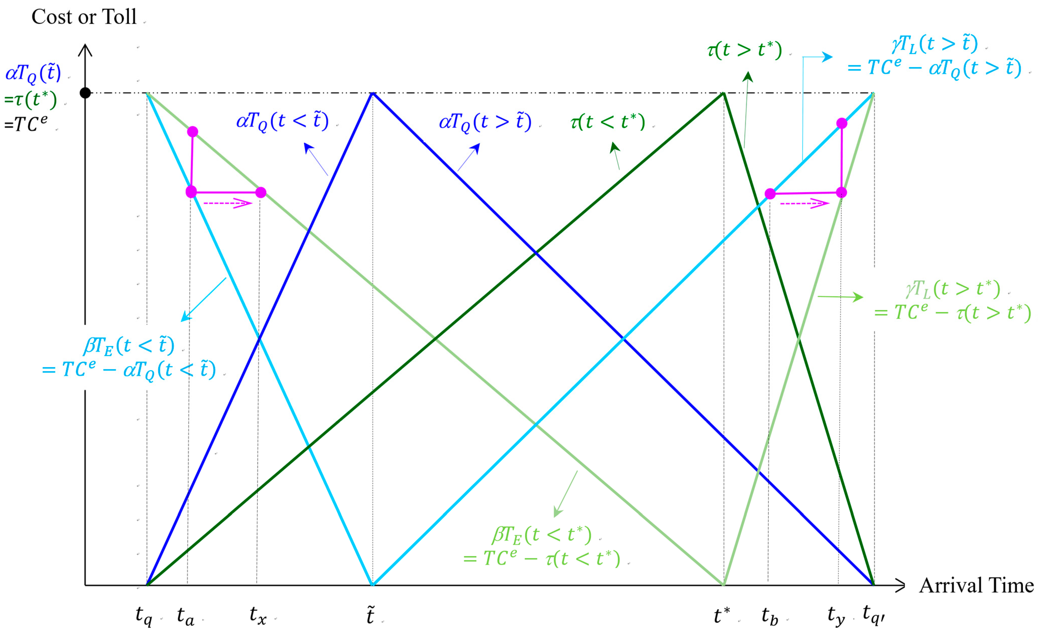
Equations (17)–(19) delineate the optimal time-varying toll scheme, denoted as $\tau \left(t\right)$, corresponding to the time-early, on-time, and time-late schedules, derived from Equations (5)–(7). It is worth noting that $\alpha T_Q\left(t\right)=0$ and $TC\left(t\right)=T{C}^e$ are two essential conditions for determining all values of $\tau \left(t\right)$. Consequently, the toll amounts ($\tau \left(t\right)$) in Equations (17)–(19) entirely substitute the queuing time cost ($\alpha T_Q\left(t\right)$) in Equations (5)–(7), while maintaining the constancy of $T{C}^e$ after toll implementation. With this toll scheme, all ships entering the canal are no longer required to queue. Instead of $\tilde{t}$ before toll implementation, $t^{*}$ emerges as the pivotal moment that distinguishes the time-early and time-late schedules for all tolled ships.

Equations (17)–(19) reveal that $\tau \left(t\right)$ linearly increases from $t_q$ to its maximum at $t^{*}$ with a slope of $\beta$. Then, it linearly decreases from $t^{*}$ to $t_{q^{\prime }}$ with a slope of −$\gamma$. Notably, as $\gamma$ surpasses $\beta$ and both are positive, $\tau \left(t\right)$ for the time-late schedule exhibits a steeper slope compared to the time-early schedule. The optimal time-varying toll scheme is meticulously designed to ensure that toll revenue precisely offsets the total queuing time cost in the equilibrium state, and effectively eliminate the need for ships to queue for canal entry. Furthermore, it is evident from Equations (17)–(19) that ships arriving at the anchorage at $t^{*}$ and making the maximum toll payment ($\tau \left(t^{*}\right)$) could enter the canal punctually at 23:00 without incurring any schedule delay costs, thereby removing costs associated with early or late entry into the canal.

4. Derivation of the Mathematical Formulas for the Arrival Times of All Tolled Ships

4.1. Motivation for the Derivation of the Mathematical Formulas

In Section 3, we explored the effectiveness of the optimal time-varying toll scheme, which successfully eradicates queuing time for all ships in the anchorage area. As a result, ships can smoothly enter the canal without enduring waiting queues. However, the existing literature lacks an in-depth examination of the specific behavioral responses that ships may exhibit after the implementation of this toll scheme, while maintaining their cost equilibrium as they were in the pre-toll scenario. To bridge this research gap, this paper presents mathematical formulas that capture how all ships adjust their arrival times at the anchorage area of the Suez Canal after the implementation of the optimal time-varying toll scheme. These formulas represent the necessary adjustments in arrival times for all tolled ships to maintain the same equilibrium cost as they had prior to the toll implementation. With the differential toll rates facilitating highly effective and evenly distributed arrival times, the toll scheme maximizes efficiency in eliminating queuing in the anchorage area.

4.2. Methodology for Deriving Mathematical Formulas

In the queuing pricing model, the equilibrium cost for each bottleneck user remains constant both before and after toll implementation, which is also known as the principle of cost equilibrium conservation. This principle is aimed at ensuring that users are not disadvantaged or incur losses after being tolled. If costs for users increase after toll implementation and exceed the equilibrium costs, it would lead to cost losses for the tolled users, potentially hindering user support for queuing pricing. As discussed in Section 3, the optimal time-varying toll scheme generates toll revenue that precisely matches the overall cost incurred by ships due to queuing times in the anchorage area. Consequently, after implementing the optimal time-varying toll scheme in the Suez Canal’s anchorage area, the costs associated with early or late arrival at the anchorage area for tolled ships must be equal to their respective costs before toll implementation, in order to adhere to the principle of cost equilibrium conservation.

As illustrated in Figure 2, the left-side dark blue triangle represents the queuing time costs of ships in the canal’s anchorage area before toll implementation $(\alpha T_Q\left(t<\tilde{t}\right)$ and $\alpha T_Q\left(t>\tilde{t}\right))$. Conversely, the corresponding light blue inverted triangle represents the early arrival time cost ($\beta T_E(t<\tilde{t})=T{C}^e-\alpha T_Q(t<\tilde{t})$) and late arrival time cost ($\beta T_L(t>\tilde{t})=T{C}^e-\alpha T_Q(t>\tilde{t})$) for these ships. These costs are incurred when the ships enter the canal before or after the designated latest entry time ($t^{*}$). On the right side of Figure 2, the dark green triangle represents the optimal time-varying tolls ($\tau (t<t^{*})$ and $\tau (t>t^{*}))$ implemented in the canal’s anchorage area. Correspondingly, the light green inverted triangle represents the early arrival time cost ($\beta T_E(t<t^{*})=T{C}^e-\tau (t<t^{*})$) and late arrival time cost ($\gamma T_L(t>t^{*})=T{C}^e-\tau (t>t^{*})$) for the tolled ships.

In Figure 2, concerning ships with the time-early schedule, those arriving at the anchorage area at $t_a$ before toll implementation will defer their arrival times until $t_x$ after toll implementation. This adjustment becomes imperative as the early arrival time cost at $t_a$ before toll implementation $\left(\beta T_E\left(t_a\right)=T{C}^e-\alpha T_Q(t_a\right))$ equals the early arrival time cost at $t_x$ after toll implementation $\left(\beta T_E\left(t_x\right)=T{C}^e-\tau (t_x\right))$. Consequently, these ships must postpone their original anchorage arrival time to $t_x$ to ensure adherence to the principle of cost equilibrium conservation. Similarly, for ships with the time-late schedule, those arriving at the anchorage area at $t_b$ before toll implementation will defer their arrival times until $t_y$ after toll implementation. This adjustment is also imperative since the late arrival time cost before toll implementation $\left(\gamma T_L\left(t_b\right)=T{C}^e-\alpha T_Q(t_b\right))$ equals the late arrival time cost at $t_y$ after toll implementation $\left(\gamma T_L\left(t_y\right)=T{C}^e-\tau (t_y\right))$. Hence, these ships must postpone their original anchorage arrival time to $t_y$ to ensure compliance with the principle of cost equilibrium conservation.

4.3. Derivation Result of the Mathematical Formulas

Based on Equations (8) and (9) in Section 3, it is evident in Figure 1 that the slopes of $\alpha T_Q(t<\tilde{t})$ and $\alpha T_Q\left(t>\tilde{t}\right)$ are $\frac{\alpha \beta }{\alpha -\beta }$ and $\frac{-\alpha \gamma }{\alpha +\gamma }$ respectively. Consequently, the slopes of $\beta T_E\left(t<\tilde{t}\right)=T{C}^e-\alpha T_Q\left(t<\tilde{t}\right)$ and $\gamma T_L\left(t>\tilde{t}\right)=T{C}^e-\alpha T_Q\left(t>\tilde{t}\right)$ are $\frac{-\alpha \beta }{\alpha -\beta }$ and $\frac{\alpha \gamma }{\alpha +\gamma }$, respectively. Furthermore, referring to Equations (17) and (19), it can be deduced that the slopes of $\tau (t<t^{*})$ and $\tau (t>t^{*})$ in Figure 2 are β and −γ, respectively. Thus, the slopes of $\beta T_E(t<t^{*})=T{C}^e-\tau (t<t^{*})$ and $\gamma T_L\left(t>\tilde{t}\right)=T{C}^e-\alpha T_Q\left(t>\tilde{t}\right)$ are $-\beta$ and γ, respectively.

In the context of an equilibrium state before toll implementation, let us assume that the arrival time of a ship entering the canal before the latest allowed entry time ($t^{*}$) is denoted as $t_a$ (where $t_q\le t_a\le \tilde{t}$). As with the earlier analysis, after the toll implementation, the ship’s arrival time at the anchorage area will be deferred to $t_x$. Based on Figure 2, we express the correlation between $t_x$ and $t_a$ as follows:

$$\begin{array}{l}-\beta \left(t_a-t_x\right)=\left(T{C}^e-\mathrm{\tau }(t_a)\right)-\left(T{C}^e-\mathrm{\alpha }{T}_Q(t_a\right))\hfill \\ \hfill \end{array}$$

$$t_x=t_a-\frac{\mathrm{\tau }(t_a)-\mathrm{\alpha }{T}_Q(t_a)}{\beta }$$

$$t_x=t_a-\frac{T{C}^e-\beta (t^{*}-t_a)-\frac{\alpha \beta }{\alpha -\beta }(t_a-t_q)}{\beta }$$

$$t_x=t^{*}+\frac{\alpha }{\alpha -\beta }(t_a-t_q)-\frac{T{C}^e}{\beta }$$

(20)

Similarly, suppose the arrival time of a ship entering the canal beyond the latest allowed entry time ($t^{*}$) is denoted as $t_b$ (where $\tilde{t}\le t_b \le t_{q\prime })$. After the toll implementation, the ship’s arrival time at the anchorage area will be deferred to $t_y$. Consequently, we express the correlation between $t_y$ and $t_b$ in Figure 2 as follows:

$$\begin{array}{l}\frac{\alpha \gamma }{\alpha +\gamma }\left(t_y-t_b\right)=\left(T{C}^e-\mathrm{\alpha }{T}_Q(t_y)\right)-\left(T{C}^e-\mathrm{\tau }(t_y\right))\hfill \\ \hfill \end{array}$$

$$t_y=t_b+\frac{\mathrm{\tau }(t_y)-\mathrm{\alpha }{T}_Q(t_y)}{\frac{\alpha \gamma }{\alpha +\gamma }}$$

$$t_y=t_b+\frac{T{C}^e-\gamma \left(t_y-t^{*}\right)+\frac{\alpha \gamma }{\alpha +\gamma }(t_y-t_{q\prime })}{\frac{\alpha \gamma }{\alpha +\gamma }}$$

$$t_y=t^{*}+\frac{\alpha }{\alpha +\gamma }(t_b-t_{q^{\prime }})+\frac{T{C}^e}{\gamma }$$

(21)

By employing the Point-Slope Form, we can formulate two mathematical formulas of Equations (20) and (21) to illustrate how all ships, after implementing the optimal time-varying toll scheme, adjust their pre-toll arrival times to eliminate queueing at the canal’s anchorage area. The derivation of these equations is based on the principle of cost equilibrium conservation, where all ships incur the same early (or late) arrival time cost both before and after toll implementation to preserve an unaltered equilibrium cost ($T{C}^e$). It is evident that these two formulas represent the adjusted arrival times at the anchorage area for two categories of tolled ships: those entering the canal before the latest allowed entry time ($t^{*}$) and those entering the canal after $t^{*}$. This adjustment described is imperative for all tolled ships to maintain their initial equilibrium of $T{C}^e$.

From Figure 2, it is evident that Equations (20) and (21) represent pre-toll arrival times on the light blue early (or late) arrival time cost (=$T{C}^e-\alpha T_Q\left(t\right)$) will be shifted to the corresponding post–toll arrival times on the light green early (or late) arrival time cost (=$T{C}^e-\tau \left(t\right)$). For instance, referring to Figure 2, if the pre-toll arrival time of ships that enter the canal earlier (or later) than the latest allowed entry time ($t^{*}$) is assumed to be $t_a$ (or $t_b$), then their post-toll arrival times will be deferred to $t_x$ (or $t_y$).

It is apparent from Figure 2 that only tolled ships with arrival times of $t_q$ and $t_{q\prime }$ maintain their original arrival times before toll implementation. Notably, the closer a tolled ship’s arrival time is to $t^{*}$, the longer the duration of delay in its arrival time. Furthermore, Figure 2 distinctly illustrates that if a ship’s arrival time coincides with $\tilde{t}$ before toll implementation, its arrival time will be deferred to $t^{*}$ after toll implementation. This can be verified by substituting $t_a=t_b=\tilde{t}$ into Equations (20) and (21), yielding $t_x=t_y=t^{*}$. This represents the longest postponement in arrival time among all tolled ships, with a value of $t^{*}-\tilde{t}=\frac{\beta \gamma }{\alpha \left(\beta +\gamma \right)}\cdot \frac{N}{S}=\frac{T{C}^e}{\alpha }=\frac{\alpha T_Q\left(\tilde{t}\right)}{\alpha }=\frac{\tau (t^{*})}{\alpha }$.

Based on the previously mentioned results, we can summarize the mathematical formula for $t_x=f(t_a)$ from Equation (20) and the other formula for $t_y=f(t_b)$ from Equation (21) in

Table 1. Mathematical formulas for the post-toll arrival times ($t_x$ and $t_y$) of all ships.

	Post-Toll	$t_x=f(t_a) \left(t_q\le t_x\le t^{*}\right)$	$t_y=f(t_b) \left(t^{*}<t{ }_y\le t_{q\prime }\right)$
Pre-Toll
$t_a \left(t_q\le t_a\le \tilde{t}\right)$		$t_x=t^{*}+\frac{\alpha }{\alpha -\beta }(t_a-t_q)-\frac{T{C}^e}{\beta }$	-
$t_b \left(\tilde{t}<t_b\le t_{q\prime }\right)$		-	$t_y=t^{*}+\frac{\alpha }{\alpha +\gamma }(t_b-t_{q^{\prime }})+\frac{T{C}^e}{\gamma }$

. Notably, the pre-toll arrival times serve as independent variables in these formulas, while the post-toll arrival times act as dependent variables. To determine the function values of the post-toll arrival times ($t_x$ and $t_y$) based on the relationship in Table 1, it is imperative to assume the pre-toll arrival times ($t_a$ and $t_b$) as given values. This assumption is both reasonable and justified because $t_a$ and $t_b$ represent the pre-toll arrival times in the equilibrium state, representing outcomes attained in a stable condition devoid of additional regulations.

4.4. Novelty in the Research Method and Its Results

The representative papers in the existing literature on queuing pricing for the Suez Canal are notably represented by Laih et al. [2] and Sun and Laih [3]. Laih et al. [2] were the first to establish a queuing pricing model for ships queuing at the Suez canal’s anchorage area. Their approach involved employing analytical mathematics method to compute the equilibrium cost for each ship and derive an optimal time-varying toll scheme, specifying the toll amounts along with corresponding start and end tolling times. This toll scheme effectively eliminated the inefficiency of ships queuing and waiting at the anchorage area to enter the canal.

Subsequently, Sun and Laih [3] examined the effects of the optimal time-varying toll scheme on ships’ arrivals at the canal’s anchorage area. In particular, their study investigated both pre-toll and post-toll sequential arrival times for all ships by a method of uniform arrival interval among arrivals. However, this methodology raises two debatable points. Firstly, the assumption that the intervals between ship arrivals at the anchorage area follow a uniform distribution lacks generality. Secondly, the approach of calculating all ships’ arrival times at the anchorage area as the accumulation of the same arrival interval from the queuing start time becomes problematic. This is because errors in the accumulated calculation amplify with an increasing number of ships. Consequently, the principle of cost equilibrium conservation for both pre-toll and post-toll ships cannot be satisfied.

To address the aforementioned controversies and enhance both the theoretical basis and practical significance of the optimal time-varying toll scheme for a queuing canal, this paper employs the Point-Slope Form method to derive mathematical formulas based on the principle of cost equilibrium conservation. The derived formulas in this paper represent all ships’ post-toll arrival times at the anchorage area. Notably, the pre-toll arrival times serve as independent variables in these formulas, while the post-toll arrival times act as dependent variables. The derived formulas not only meet the requirement of maintaining cost equilibrium for all tolled ships, but also contribute to maximizing efficiency in eliminating queuing in the canal’s anchorage area.

Table 2. Novelty of this paper compared to the works by Laih et al. [2] and Sun and Laih [3].

	Papers	Laih et al. [2]	Sun and Laih [3]	This Paper
Novelty
Method		Development of a Queuing Pricing Model for the Canal using Analytical Mathematics	Investigation on sequential arrive times using Uniform Arrival Interval	Exploration of arrival time adjustments using Point-Slope Form
Findings		Equilibrium cost for each pre-toll ship. Determination of optimal time-varying toll amounts along with corresponding start and end tolling times.	Determination of the average arrival interval among arrivals at the canal’s anchorage. Examination of Ships’ sequential arrival times by the accumulation of the average arrival interval from the queuing start time.	Formulation of mathematical formulas for adjusting the arrival times of all tolled ships at the canal’s anchorage. Ensuring that post-toll arrival times incur the same schedule delay costs as pre-toll arrival times to adhere to the Cost Equilibrium Conservation Principle.

compares the research methods and findings of the works by Laih et al. [2] and Sun and Laih [3], with those presented in this paper to highlight its novelty.

5. Numerical Analysis

Between 2020 and 2022, the global COVID-19 pandemic significantly impacted maritime transportation. Additionally, an unexpected incident occurred in March 2021 when a container ship ran aground in the Suez Canal, resulting in a complete blockage of traffic in both directions for approximately one week. These events had a profound effect on the regular operations of the Suez Canal, causing substantial delays in the availability of official statistical data. The most recent navigation statistics accessible on the Suez Canal’s official website [1] are currently updated only until February 2020. Consequently, we can only rely solely on statistical data throughout 2019 to simulate how tolled ships adjusted their pre-toll arrival times at the canal’s anchorage area. These results will serve as a practical reference for canal authorities when considering the implementation of an optimal time-varying toll scheme.

Referring to the statistics provided by the Suez Canal Authority for the year 2019, there were 9711 ships traversing the Suez Canal in the southbound direction towards the Red Sea, while 9169 ships traveled northbound direction towards the Mediterranean. Consequently, the average number of ships passing through per day (N) was computed as 26.61 (=9711/365) for the southbound direction and 25.12 (=9169/365) for the northbound direction. In accordance with information from the Suez Canal Authority, the specified time frames for the entry of southbound and northbound ships into the canal are as follows: Southbound ships are permitted to enter between 03:30 and 23:00, while northbound ships are allowed enter between 04:00 and 23:00. Based on this, the canal capacity (S) for the southbound and northbound directions can be calculated as 1.36 ships per hour (=26.61/19.5) and 1.32 ships per hour (=25.12/19), respectively.

The hourly queueing time cost (α) for ships awaiting entry into the Suez Canal at the anchorage area can be construed as their opportunity cost. Among the various opportunity costs incurred by ships queueing for Suez Canal entry, the most consequential for shipowners is typically the hourly rental income of a ship. Based on historical data provided by the Suez Canal Authority, container ships constitute the predominant category among all transiting ships. Therefore, the calculation of the value α will be grounded in the rental rates applicable to container ships. In 2019, the value of α will be calculated using the rental rates for container ships. In 2019, the average net tonnage of container ships passing through the canal was recorded as 118,344.37 tons. Typically, 1 TEU is equivalent to 13.6 net tons. Therefore, 118,344.37 net tons can be approximately converted to 8700 TEUs. According to data from Harper Petersen & Co. for 2019, the daily rental rate for an 8700 TEU container ship was approximately USD 25,458.33. Thus, the average hourly rental rate per container ship can be calculated as USD 1060.76 (=25,458.33/24). In summary, the hourly queueing time cost for ships awaiting entry into the Suez Canal can be considered as USD 1060.76 (α = $1060.76).

The hourly cost associated with early arrival time (β) and late arrival time (γ) for ships can be construed as their penalty costs. When a ship arrives early at the anchorage of the Suez Canal, it implies a likelihood of reaching its destination port ahead of schedule. However, this early arrival poses a tough challenge in coordinating the necessary manpower and equipment for immediate and efficient cargo handling at the destination port. As a result, the early arrival of the ship requires additional payment of berth anchorage fees until cargo operations can commence. Therefore, the berth anchorage fee can serve as the basis for computing the ship’s early arrival time cost. The computation of berth anchorage fees is based on the reference of the current container throughput of Shanghai Port, the world’s largest port, which amounts to CNY 0.25 per ton per day, approximately equivalent to USD 0.039. Thus, the hourly cost incurred for the ship’s early arrival can be computed as USD 192.31 (β = 0.039 × 118,344.37 ÷ 24 = 192.31).

Furthermore, as stipulated by the Suez Canal Authority, both southbound and northbound ships must adhere to the arrival deadline of 23:00 ($t^{*}$ = 23) to gain entry into the canal. In cases of late arrivals, canal authorities impose varying charges: a maximum of 12,500, 25,000, and 30,000 Special Drawing Rights (SDR) for the respective time periods of 23:00–00:00, 00:00–01:00, and 01:00–. Calculating the average of these amounts results in 22,500 SDR (approximately equal to USD 31,515.75), representing the penalty cost for the ship’s delay. Therefore, the cost of late arrival time per ship is computed as USD 1313.16 per hour (γ = 31,515.75/24 = 1313.16).

By substituting the aforementioned values into Equation (16) provided in Section 3, we determine the equilibrium costs ($T{C}^e$) per southbound and northbound ship to be USD 3282.75 and USD 3192.17, respectively. Additionally, applying Equations (13)–(15) allows us to obtain that $t_q$ = 5.97 = 5:58, $\tilde{t}$ = 19.87 = 19:52 and $t_{q^{\prime }}$ = 25.54 = 01:32 for southbound ships, as well as $t_q$ = 6.44 = 6:26, $\tilde{t}$ = 19.96 = 19:58 and $t_{q^{\prime }}$ = 25.47 = 01:28 for northbound ships. From these results, it is apparent that a significant proportion of both southbound and northbound ships enter the canal before the specified time of 23:00. In addition, only southbound and northbound ships arriving at the anchorage area at $\tilde{t}$ = 19.87 = 19:52 and $\tilde{t}$ = 19.96 = 19:58, respectively, can enter the Suez Canal at the permissible latest time of 23:00 ($t^{*}$ = 23).

Under the optimal time-varying toll scheme implemented in the anchorage area of Suez Canal, the total daily revenue ($\tau \left(t^{*}\right)·(t_{q^{\prime }}-t_q)/2)·S$ for southbound and northbound ships is $43,685.52 and $40,093.02, respectively. These total revenue amounts precisely match the total queueing time costs for southbound and northbound ships before the toll implementation. This means that the total toll collected completely offsets the total queueing time costs, eliminating the need for ships to wait in a queue before entering the canal under the optimal time-varying toll scheme. Therefore, tolled ships arriving at the anchorage area prior to the specified time of $t^{*}$ = 23 will be granted entry into the Suez Canal at an earlier time, while the remaining tolled ships arriving after $t^{*}$ = 23 will experience a delay in entering the canal beyond the stipulated entry time. Southbound (or northbound) ships arriving precisely at $t^{*}$ = 23 must be tolled a maximum amount of $\tau \left(t^{*}\right)$ = USD 3282.75 (or USD 3192.17) to avoid incurring additional costs for early or delayed entry into the canal.

Table 3. Numerical results for southbound ships from the pre-toll to the post-toll scenario.

Southbound Ships
Pre-Toll			Toll	Post-Toll			Extension of t
$t=t_a,t_b$ (am/pm)	$T_Q\left(t\right)$ (h)	$t+T_Q\left(t\right)$ (am/pm)	$\tau \left(t\right)=\alpha T_Q\left(t\right)$ (USD)	$t=t_x,t_y$ (am/pm)	$T_Q\left(t\right)$ (h)	$t+T_Q\left(t\right)$ (am/pm)	$\Delta t=t_x-t_a$ (h) $\Delta t=t_y-t_b$(h)
05.97 ($t_q$)	0.00	05.97	0.00	05.97 ($t_q$)	0.00	05.97	0.00
:	:	:	:	:	:	:	:
07.00	0.19	07.19	201.54	07.19	0.00	07.19	0.19
:	:	:	:	:	:	:	:
08.00	0.41	08.41	434.91	08.41	0.00	08.41	0.41
:	:	:	:	:	:	:	:
09.00	0.63	09.63	668.28	09.63	0.00	09.63	0.63
:	:	:	:	:	:	:	:
10.00	0.85	10.85	901.65	10.85	0.00	10.85	0.85
:	:	:	:	:	:	:	:
11.00	1.07	12.07	1135.01	12.07	0.00	12.07	1.07
:	:	:	:	:	:	:	:
12.00	1.29	13.29	1368.38	13.29	0.00	13.29	1.29
:	:	:	:	:	:	:	:
13.00	1.51	14.51	1601.75	14.51	0.00	14.51	1.51
:	:	:	:	:	:	:	:
14.00	1.73	15.73	1835.11	15.73	0.00	15.73	1.73
:	:	:	:	:	:	:	:
15.00	1.95	16.95	2068.48	16.95	0.00	16.95	1.95
:	:	:	:	:	:	:	:
16.00	2.17	18.17	2301.85	18.17	0.00	18.17	2.17
:	:	:	:	:	:	:	:
17.00	2.39	19.39	2535.22	19.39	0.00	19.39	2.39
:	:	:	:	:	:	:	:
18.00	2.61	20.61	2768.58	20.61	0.00	20.61	2.61
:	:	:	:	:	:	:	:
19.00	2.83	21.83	3001.95	21.83	0.00	21.83	2.83
:	:	:	:	:	:	:	:
19.87 ($\tilde{t}$)	3.13	23.00	3320.18	23.00 ($t^{\mathrm{*}}$)	0.00	23.00	3.13
:	:	:	:	:	:	:	:
21.00	2.46	23.46	2609.47	23.46	0.00	23.46	2.46
:	:	:	:	:	:	:	:
22.00	1.91	23.91	2026.05	23.91	0.00	23.91	1.91
:	:	:	:	:	:	:	:
23.00 ($t^{\mathrm{*}}$)	1.36	24.36	1442.63	24.36	0.00	24.36	1.36
:	:	:	:	:	:	:	:
24.00	0.81	24.81	859.22	24.81	0.00	24.81	0.81
:	:	:	:	:	:	:	:
25.00	0.26	25.26	275.80	25.26	0.00	25.26	0.26
:	:	:	:	:	:	:	:
25.54 ($t_{q\prime }$)	0.00	25.54	0.00	25.54 ($t_{q\prime }$)	0.00	25.54	0.00

and Figure 3, as well as

Table 4. Numerical results for northbound ships from the pre-toll to the post-toll scenario.

Northbound Ships
Pre-Toll			Toll	Post-Toll			Extension of t
$t=t_a,t_b$ (am/pm)	$T_Q\left(t\right)$ (h)	$t+T_Q\left(t\right)$ (am/pm)	$\tau \left(t\right)=\alpha T_Q\left(t\right)$ (USD)	$t=t_x,t_y$ (am/pm)	$T_Q\left(t\right)$ (h)	$t+T_Q\left(t\right)$ (am/pm)	$\Delta t=t_x-t_a$ (h) $\Delta t=t_y-t_b$(h)
06.44 ($t_q$)	0.00	06.44	0.00	06.44 ($t_q$)	0.00	06.44	0.00
:	:	:	:	:	:	:	:
07.00	0.09	07.09	95.47	07.09	0.00	07.09	0.09
:	:	:	:	:	:	:	:
08.00	0.31	08.31	328.84	08.31	0.00	08.31	0.31
:	:	:	:	:	:	:	:
09.00	0.53	09.53	562.20	09.53	0.00	09.53	0.53
:	:	:	:	:	:	:	:
10.00	0.75	10.75	795.57	10.75	0.00	10.75	0.75
:	:	:	:	:	:	:	:
11.00	0.97	11.97	1028.94	11.97	0.00	11.97	0.97
:	:	:	:	:	:	:	:
12.00	1.19	13.19	1262.30	13.19	0.00	13.19	1.19
:	:	:	:	:	:	:	:
13.00	1.41	14.41	1495.67	14.41	0.00	14.41	1.41
:	:	:	:	:	:	:	:
14.00	1.63	15.63	1729.04	15.63	0.00	15.63	1.63
:	:	:	:	:	:	:	:
15.00	1.85	16.85	1962.41	16.85	0.00	16.85	1.85
:	:	:	:	:	:	:	:
16.00	2.07	18.07	2195.77	18.07	0.00	18.07	2.07
:	:	:	:	:	:	:	:
17.00	2.29	19.29	2429.14	19.29	0.00	19.29	2.29
:	:	:	:	:	:	:	:
18.00	2.51	20.51	2662.51	20.51	0.00	20.51	2.51
:	:	:	:	:	:	:	:
19.00	2.73	21.73	2895.87	21.73	0.00	21.73	2.73
:	:	:	:	:	:	:	:
19.96 ($\tilde{t}$)	3.04	23.00	3224.71	23.00 ($t^{*}$)	0.00	23.00	3.04
:	:	:	:	:	:	:	:
21.00	2.41	23.41	2556.43	23.41	0.00	23.41	2.41
:	:	:	:	:	:	:	:
22.00	1.86	23.86	1973.01	23.86	0.00	23.86	1.86
:	:	:	:	:	:	:	:
23.00 ($t^{*}$)	1.31	24.31	1389.60	24.31	0.00	24.31	1.31
:	:	:	:	:	:	:	:
24.00	0.76	24.76	806.18	24.76	0.00	24.76	0.76
:	:	:	:	:	:	:	:
25.00	0.21	25.21	222.76	25.21	0.00	25.21	0.21
:	:	:	:	:	:	:	:
25.47 ($t_{q\prime }$)	0.00	25.47	0.00	25.47 ($t_{q\prime }$)	0.00	25.47	0.00

and Figure 4, predominantly illustrate the variations in arrival times at the anchorage area of Suez Canal for both southbound and northbound ships after implementing the optimal time-varying toll scheme. In Table 3 and Table 4 (or Figure 3 and Figure 4), the colored values (or dots) in green and red represent the results for time-early (including on-time) and time-late schedules, respectively.

The “Pre-Toll” column in Table 3 and Table 4 consists of three rows. The first row illustrates the arrival times ($t$) at the anchorage area of the Suez Canal before toll implementation. These times fall within the queueing start time ($t_q$) and the queueing end time ($t_{q\prime }$) in the pre-toll equilibrium situation. The second row displays the corresponding queueing time length ($T_Q\left(t\right)$) for each arrival time $\left(t\right)$. The values in green and red are computed using $T_Q\left(t\right)=\left(t-t_q\right)\frac{\beta }{\alpha -\beta }$ and $T_Q\left(t\right)=\left(t-t_{q^{\prime }}\right)\frac{-\gamma }{\alpha +\gamma }$, respectively. The third row presents the sum of the first and second rows, indicating the time at which the ship enters the canal after queueing at the anchorage area.

In the “Toll” column of Table 3 and Table 4, the optimal time-varying toll amount ($\tau \left(t\right)$) is determined using Equations (17)–(19) in Section 3. Since $\left(t\right)$ fully offsets 100% of the queueing time cost, it can also be considered as $\alpha T_Q\left(t\right)$. This implies that by multiplying USD 1060.76 (=α) by the values of $T_Q\left(t\right)$ corresponding to all arrival times before toll implementation, we obtain the optimal toll amount that each arriving ship should be tolled to eliminate the queueing time cost.

The “Post-Toll” column in Table 3 and Table 4 consists of three rows. The first row illustrates the arrival times, $t_x$ and $t_y$, for all the tolled ships computed using the two mathematical formulas (Equations (20) and (21)) in Section 4. Under the optimal time-varying toll scheme, the values in the second row are all zero since the queueing time corresponding to each arrival time disappears ($T_Q\left(t_x\right)=T_Q\left(t_y\right)=0$). The third row represents the times when all the tolled ships enter the canal, and all values are the same as those in the first row since there is no queuing after toll implementation.

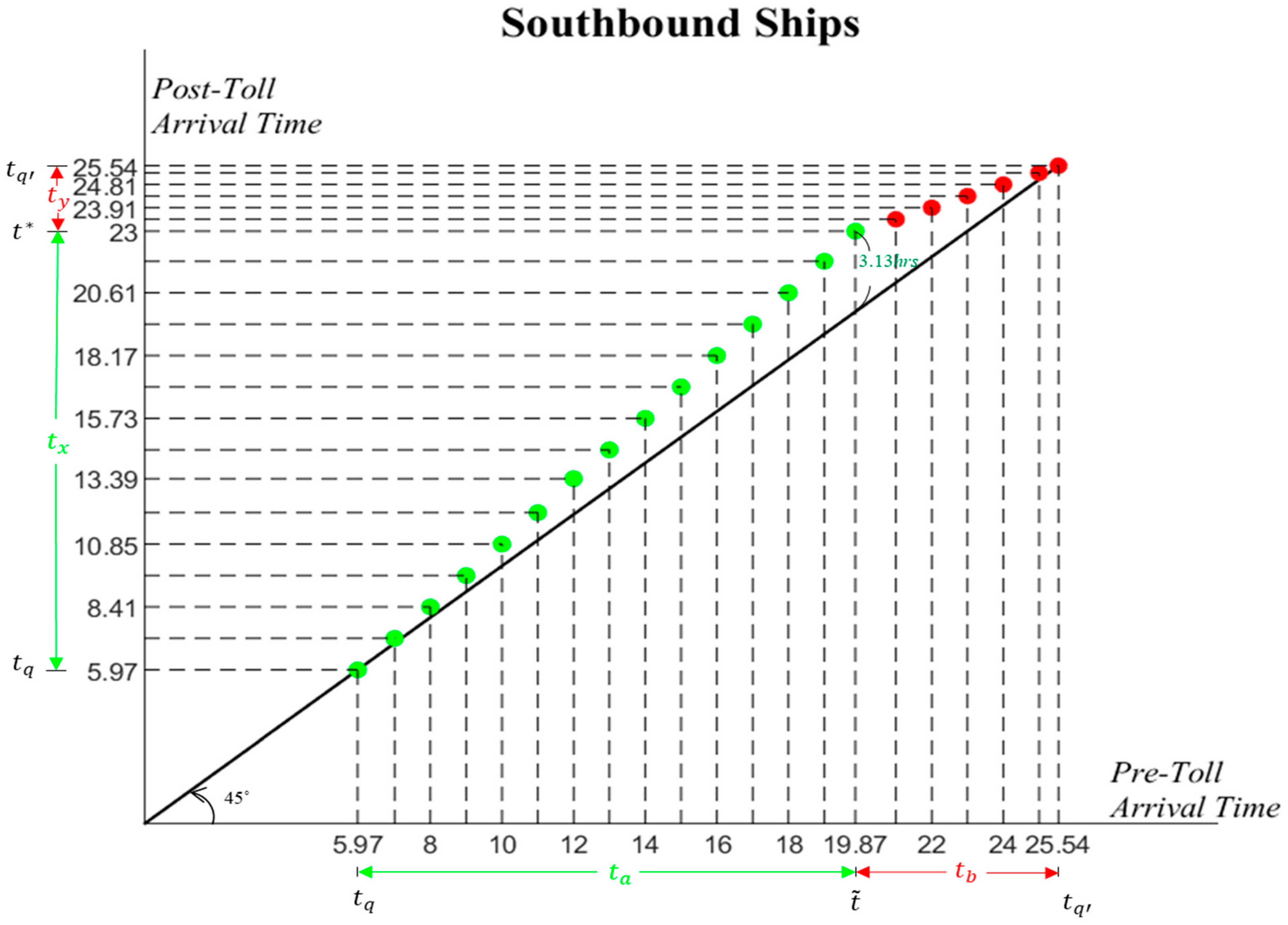
In the “Extension of $t$” column of Table 3 and Table 4, the duration (Δt) by which the arrival times of all tolled ships are deferred compared to their pre-toll arrival times can be determined by subtracting the arrival times before toll implementation ($t$ = $t_a$ and $t_b$) from the arrival times after toll implementation ($t$ = $t_x$ and $t_y$). Taking the southbound ships in Table 3 as an example, it becomes evident that for the early arrival time interval ($t_q=5.97,\tilde{t}=19.87$) before toll implementation, all arrival times exhibit an increasing postponement in arrival time (green Δt = 0~3.13 h) after toll implementation. Additionally, there is a marginal increase of +0.22 h in the deferred duration at every full hour between $t_q=5.97$ and $\tilde{t}=19.87$. At the arrival time $\tilde{t}=19.87$, the longest postponement in arrival time is observed, approximately 3.13 h. Conversely, during the delayed arrival time interval ($\tilde{t}=19.87,t_{q\prime }=25.54$) before toll implementation, all arrival times show a decreasing postponement in arrival time (red Δt = 3.13 to 0 h) after toll implementation. Furthermore, a marginal reduction of −0.55 h in the deferred duration is observed at every full hour between $\tilde{t}=19.87$ and $t_{q\prime }=25.54$.

Figure 3 presents the findings from Table 3, depicting that only two southbound untolled ships with arrival times of $t_q=5.97$ and $t_{q\prime }=25.54$ do not necessitate adjustments to their pre-toll arrival times, hence they lie on the 45-degree line. However, all other southbound tolled ships arriving between $t_q=5.97$ and $t_{q\prime }=25.54$ need adjustments to their pre-toll arrival times to maintain cost equilibrium. The green dots, representing time-early arrivals, gradually deviate from the 45-degree line (indicating an increasing postponement in arrival time) over time. The highest tolled ship, arriving at $\tilde{t}=19.87$, is positioned farthest from the 45-degree line (with a longest postponement of 3.13 h). Conversely, the red dots, corresponding to time-late arrivals, gradually approach the 45-degree line (indicating a decreasing postponement in arrival time approaching zero) over time until the end of queuing.

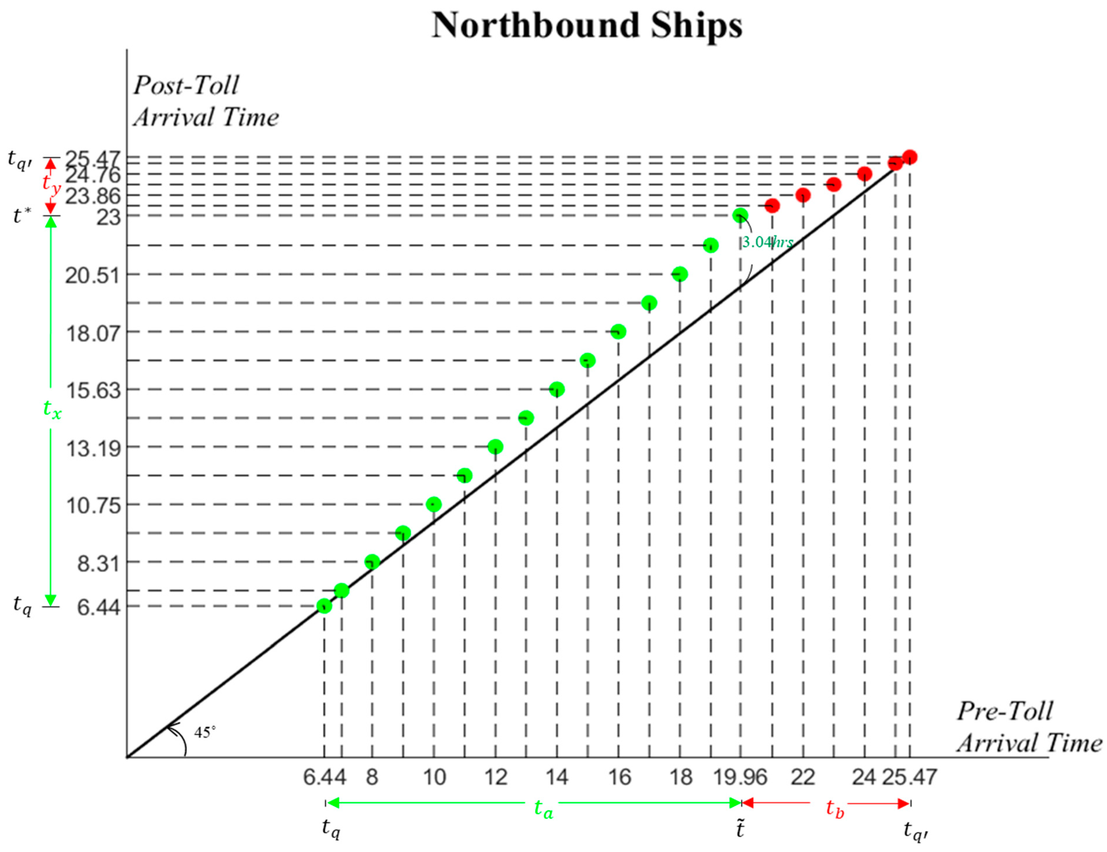
The values in Table 4 demonstrate slight differences compared to Table 3, which is primarily attributed to minor variations in the values of $t_q$, $\tilde{t}$, $t_{q\prime }$, N, and S for the northbound and southbound directions. However, when it comes to the marginal postponement in arrival time at every full hour for northbound tolled ships, Table 4 reflects identical values as Table 3. This implies that the marginal postponement in arrival time for both southbound and northbound ships is +0.22 and −0.55 h, respectively, during the early and delayed arrival time intervals. Regarding the variation in arrival times for all northbound tolled ships in Table 4, please refer to the proximity of the green and red dots to the 45-degree line in Figure 4. The highest tolled ship with an arrival time of $\tilde{t}=19.96$ deviates the farthest from the 45-degree line (approximately 3.04 h), indicating the longest postponement in arrival time after toll implementation.

The above provided information can serve as a valuable reference for canal authorities in planning the quantity and configuration of relevant hardware and software equipment. Additionally, it can aid in the scheduling of canal pilots, especially when considering the implementation of the optimal time-varying toll scheme.

6. Conclusions

The optimal time-varying toll scheme is specifically designed to eliminate ship queuing at the anchorage area and enhance efficient utilization of the canal. This toll scheme differs significantly from the current tolling system in the Suez Canal, which primarily aims at covering management and operational costs through user payments. Despite this contrast, the existing literature has not thoroughly explored the potential impact of implementing the optimal time-varying toll scheme on the arrival times of all tolled ships at the the Suez Canal’s anchorage area. Changes in arrival times under this toll scheme will lead to the redistribution of schedule delay costs (the penalty costs for either early or late entry into the canal) for all tolled ships while maintaining their equilibrium costs, thereby achieving maximum efficiency in eradicating queuing issues at the canal anchorage area.

As the total queuing time costs are completely offset by the revenue generated from the optimal time-varying toll scheme, all ships, both before and after toll implementation, must maintain the same schedule delay cost to achieve the principle of cost equilibrium conservation. To attain this objective, this paper utilizes the Point-Slope Form to derive two concise and comparative mathematical formulas for calculating the arrival times of all tolled ships at the Suez Canal’s anchorage area. These derived formulas not only enhance the theoretical foundation of the existing pricing model for a queuing canal, but also facilitate the electronic management of ship arrival time information for canal authorities implementing this toll scheme.

These two derived formulas represent the post-toll arrival times at the anchorage area for two distinct categories of tolled ships: those entering the canal before the specified latest entry time of 23:00 and those entering thereafter. Upon comparing these results with their pre-toll arrival times, it is evident that, for tolled ships entering the canal before 23:00, the duration of their postponement in arrival time gradually increases from zero until they precisely enter the canal at 23:00, coinciding with the time of the maximum toll amount. The deferred duration for ships entering the canal at 23:00 is the longest, identical to the maximum toll amount (or the equilibrium cost) divided by the hourly queuing time cost. Conversely, for ships entering the canal later than 23:00, the duration of their postponement in arrival time decreases until it reaches zero at the end of the queuing time.

Presently, the latest available navigation statistics on the Suez Canal’s official website are only updated until February 2020. Consequently, our numerical analysis relies on the statistical data for the entire year of 2019 to simulate the potential changes in arrival times at the Suez Canal’s anchorage area for both southbound and northbound ships under the optimal time-varying toll scheme. Using the two mathematical formulas derived from the Point-Slope Form, we calculate the post-toll arrival times for both southbound and northbound ships. By comparing these arrival times with their respective pre-toll arrival times, we can determine the postponement in arrival times experienced by tolled ships in both southbound and northbound directions. This information serves as a valuable reference for canal authorities when considering the adoption of the optimal time-varying toll scheme. It also aids in the strategic planning of resource allocation necessary for this toll scheme’s implementation. For instance, these resources may involve scheduling canal pilots effectively when the toll scheme takes effect.