1. Introduction
The broader industry is currently undergoing transformative shifts that align with the Fourth Industrial Revolution, widely recognized as Industry 4.0. This significant industrial progression is primarily propelled by the enhancement of resource management within production processes through data utilization. As a result, companies are actively embracing digital transformation to unlock heightened value.
Within the naval industry, the concept of Industry 4.0 has evolved into more distinct terms like Shipyard 4.0 [
1] and Port 4.0 [
2]. It is essential to emphasize that Industry 4.0 encompasses more than just the production phase of products (in this context, referring to ships and other maritime items); it encompasses tracking a product throughout its lifecycle and even into material recycling post-use. This ideology has given rise to remote inspections as well. Given the inevitability of digital transformation for numerous enterprises, not solely shipyards, the term Industry 4.0 is employed as a comprehensive descriptor within this paper.
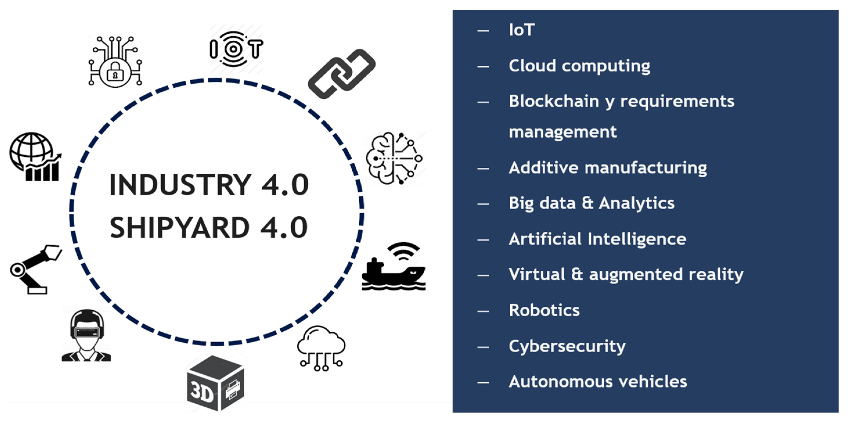
The distinctive aspect of Industry 4.0, in contrast to prior revolutions, is its multi-pronged approach, depicted in
Figure 1. These diverse facets of progress do not advance uniformly; while certain areas have experienced rapid evolution, others have undergone more gradual shifts.
The interconnected nature of these facets adds to their intrigue as an advancement in one realm can trigger improvements in others. Nevertheless, it is crucial to recognize that these facets are distinct since they pertain to varying modes of data manipulation and treatment.
The marine sector represents a strategic domain of considerable complexity, as a ship’s impact extends beyond its mere construction to subsequent operational phases. This implies that various factors come into play, including the vessel’s intended operating location, prevailing national policies, global diplomatic relations, climate considerations, ongoing regulations, and more.
A ship’s lifecycle spans approximately 20–25 years. Given their extended operational span, ships often undergo maritime transformations, such as extensions in length or beam, alterations to primary and auxiliary machinery systems, and similar modifications. These transformations can lead to deviations from the cost projections made during the initial design phase of a ship. Industry 4.0 is poised to facilitate the development of more effective strategies through data analysis, ultimately resulting in reduced expenses.
The wealth of ship-related data, ranging from data emanating from onboard sensors to information gathered through worker-conducted surveys, previously posed a challenge due to the multitude of variables influencing it (for example, variables that measure the movement of the ship, structural resistance, and weather conditions). However, Industry 4.0 has now made it feasible to manage and harness this data effectively.
“
Among the ten most important strategic technological trends that the consulting firm Gartner has pointed out for the coming years, artificial intelligence, data analytics and digital twins stand out.” [
3] (cited in [
4] p. 45).
The job displacement attributed to Industry 4.0 is closely linked to the workforce aboard autonomous ships, often referred to as smart ships. The introduction of unmanned engine rooms and checkpoints will undoubtedly yield a substantial impact on employment. However, it is vital not to overlook the intricate nature of the Industry 4.0 landscape and smart ships. Consequently, skilled personnel will be indispensable for managing the artificial intelligence algorithms that bestow autonomy upon these ships. Additionally, a workforce will be necessary to process the ever-expanding data volume, considering its exponential growth over time.
In the maritime realm, advancements like virtual, augmented, and mixed reality have emerged, not solely for simulation purposes but also to diagnose systems or mechanisms without requiring physical disassembly. This approach leads to time and cost savings. Likewise, digital twins have found their place in this domain, serving to study ships or shipyards under various operational scenarios through simulations. The unique advantage of digital twins, as exact replicas of their digitized counterparts, lies in their ability to yield predictions closely aligned with real-world behavior. As we embrace the journey toward decarbonization, digital twins will occupy a pivotal role.
In summary, the digitalization of the maritime industry, coupled with the application of novel machine-learning methodologies, is ushering in uncharted avenues of work that are poised to revolutionize the marine sector.
2. Materials and Methods: Machine Learning and Its Algorithms
Machine learning encompasses a collection of artificial intelligence algorithms employed in data analysis, enabling machines to learn and execute tasks autonomously. This capability is pivotal for systems to effectively analyze and glean insights from extensive datasets. The ultimate aim is to enhance productivity, curtail expenses, and engender favorable outcomes for the industry.
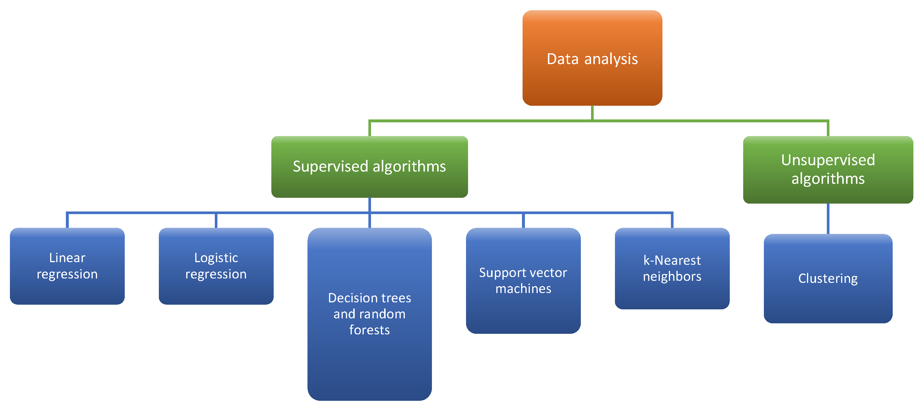
Data analysis can be broadly categorized into two distinct groups, as illustrated in
Figure 2, based on their intended objectives:
Supervised analyses: These are employed for predictive purposes and necessitate historical data for problem modeling. In this scenario, one variable is designated as the target variable, while the remaining variables function as predictor variables.
Unsupervised analyses: These are utilized for data structuring and do not rely on historical data for problem modeling. They are reliant on data extracted at the current moment, obviating the need for past behavior records (this is particularly applicable to certain classification algorithms, for instance). All variables within the dataset serve as predictor variables.
The ensuing steps in the data analysis undertaken in this paper, as well as those recommended to be followed, are elucidated in
Figure 3.
2.1. Machine Learning Algorithms
Continuing, we will delve into succinct explanations of several machine learning algorithms to provide a foundational grasp of their functions.
Machine learning methods are extensively used in the maritime industry, for example:
Prediction of ship motion and trajectory [
5].
Evaluation of navigation risk [
6].
Monitoring ship fuel consumption and optimizing ship design [
7].
Development and application of green and intelligent inland vessels [
8].
Estimation of the berthing state of autonomous maritime surface ships [
9].
Quantifying Arctic oil spill event risk [
10].
2.1.1. Linear/Nonlinear Regression
Widely adopted by the scientific community, this algorithm proves instrumental in data analysis. Input variables can span the numeric or categorical spectrum, with the latter entailing binary values: 1 if a prediction pertains to that category, and 0 otherwise.
In this context, an output variable (target variable:
) is selected, while the remaining variables act as predictors (predictor variables:
). The linear regression equation takes shape as:
where
: Represents the value attributed to the prediction within the regression process.
: Reflects the value assumed by the predictor variable (numeric or categorical).
: Denotes the coefficient termed the intercept, signifying the y-intercept within the regression equation.
: Stands for the coefficient of the input variable .
Equation (1) entails only two unknowns: the coefficients
and
. The algorithm seeks these coefficients’ values that minimize the sum of squared errors, as manifested in Equation (2).
where
: Represents the error corresponding to the -th data point concerning the regression equation.
: Stands for the value of the output variable within the dataset (i.e., the dataset’s output value).
: Signifies the database’s size, indicative of the number of elements in the dataset.
The same foundational concept extends to scenarios involving multiple variables; the key divergence is the involvement of more than one predictor variable. A parallel application pertains to nonlinear regression, where it is important to note that the resultant regression expression is not a first-degree algebraic form.
2.1.2. Clustering
Clustering, an unsupervised algorithm, operates without the need for historical data. A current database suffices for application. In this scenario, all variables are employed as inputs.
This algorithm segments data through the creation of groups containing similar elements. Both similarities and differences among the data are taken into account during this process. These groups are referred to as clusters.
The foundation for forming these groups lies in the distances between points representing individual data. The distance metric serves as a critical hyperparameter in clustering. While there are multiple ways to compute distances, for simplicity, this analysis will exclusively employ Euclidean distances, as portrayed in the general Equation (3).
where
: Represent two points for which the distance is calculated.
Subscripts or denote the respective points.
Subscript pertains to each variable.
This concept extends into three-dimensional space (each variable occupies a distinct axis:
) as depicted in Equation (4).
It is crucial to acknowledge the varying ranges of different variables, which necessitates distance normalization. This is accomplished through Equation (5).
where
: The element in the normalized database.
: The element in the unnormalized database.
: The minimum element in column of the unnormalized database.
: The maximum element in column of the unnormalized database.
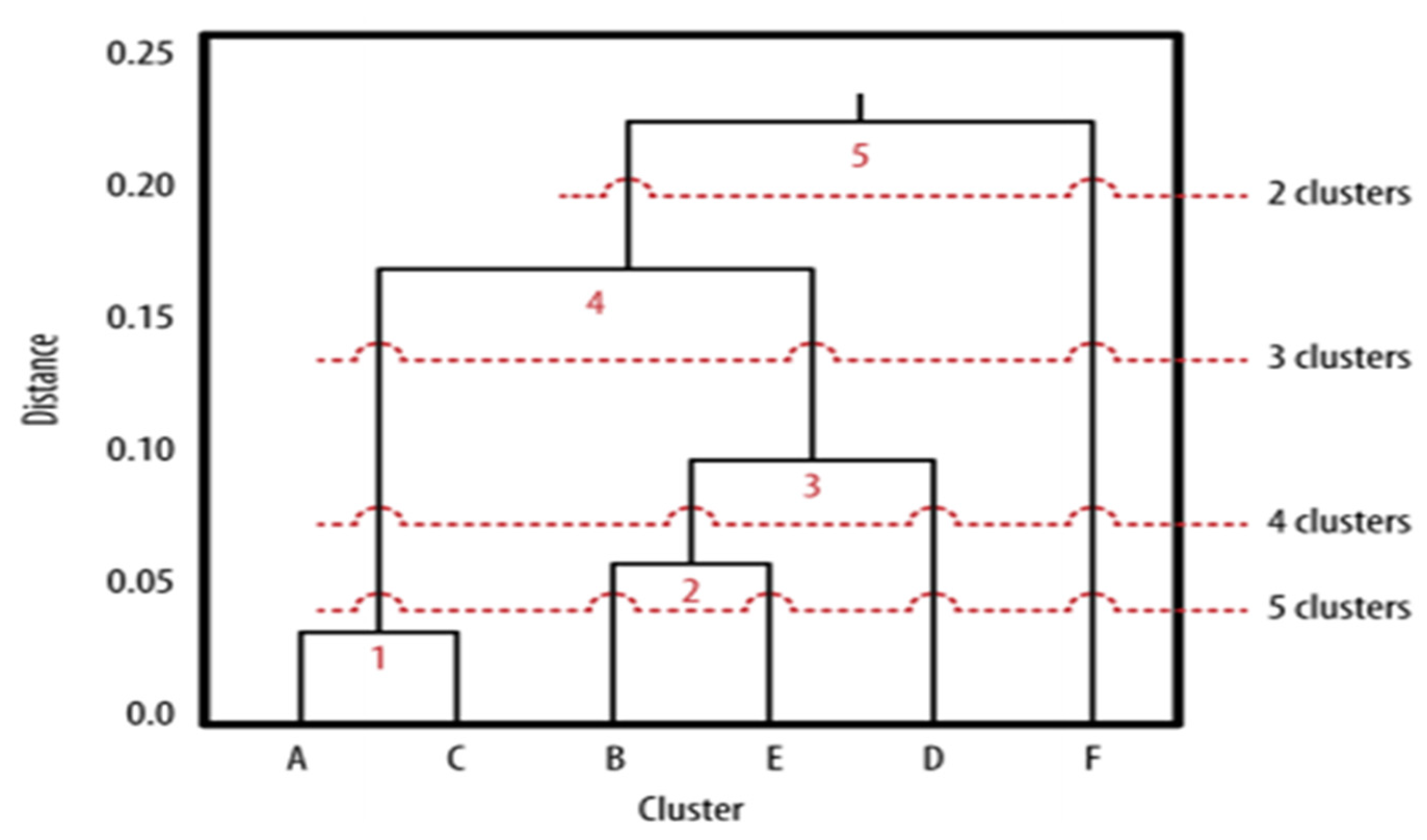
In this study, agglomerative hierarchical clustering will be employed. This algorithm initially creates n clusters (one per data point) and iteratively merges them until a predetermined number of clusters is achieved.
Hierarchical clustering is often represented visually using a dendrogram, similar to the illustration shown in
Figure 4. The positioning of a threshold holds significant importance, as it determines whether data points are organized into a larger or smaller number of clusters. Raising the threshold on the dendrogram results in fewer clusters while lowering it leads to a greater number of clusters being formed.
2.1.3. Decision Trees and Random Forests
As members of the supervised algorithm category, decision trees demand historical data for their functioning. Their core role involves data classification, a process resembling clustering. Nonetheless, a significant divergence emerges in their application intent. While clustering aims to create structural organization within data, decision trees are specifically designed for making predictions.
For a visual depiction of decision trees, please refer to
Figure 5:
As illustrated in
Figure 5, the nomenclature of this algorithm stems from its visual development, reminiscent of a tree with its branching structure.
The tree’s inception lies within a root node. At each node, decisions are made based on variable values. If a condition is met, the data branch left; failing that, the condition leads to a rightward branch. Notably, terminal nodes—also known as leaf nodes—abstain from decision-making. Instead, they furnish the final prediction.
Figure 5 underscores this concept by displaying the absence of further branches beyond these terminal nodes.
For classification tasks, it is advisable to attain maximum homogeneity within the data. Higher homogeneity reduces the information required to represent the decision tree. Homogeneity assessment employs two metrics: information entropy and information gain/loss.
The entropy formulation for a target variable is encapsulated in Equation (6):
where
: The probability of occurrence (it is the proportion occurrence of the class that is predicted since it is a statistic that is obtained by maximum likelihood) of the class .
: Number of categories for each target variable.
Every node in the tree possesses an associated information entropy value. An analogy to thermodynamic entropy reveals that the null value represents an optimal outcome, signifying a defect-free structure. The algorithm strives to minimize entropy, with zero being the ideal value. The process of entropy reduction is termed information gain, with greater reduction yielding higher information gain. Smaller entropy and greater information gain lead to more homogenous information for each target variable.
2.1.4. Regression Trees
Regression trees bear a resemblance to decision trees. Employed when the decision variable is continuous, regression trees address data with non-linear or non-logistic behavior. These trees create models to capture complex nonlinear relationships. Notably, if output variable values are missing, they can be averaged over terminal nodes.
In each node, samples are present:
The prediction is calculated as the average:
2.1.5. Random Forests
In a manner that is intuitive and can be likened to an analogy, a random forest is comprised of a fusion of multiple decision or regression trees. However, the noteworthy aspect here is that the hyperparameters (such as the minimum number of samples per node, minimum and maximum tree depth, etc.) are not rigidly set. Instead, these hyperparameters exhibit random variations for each tree constituting the forest.
Within the forest, a diversity of trees is present, some with greater depth and others with shallower depth. Similarly, there are trees with more terminal nodes, and those with fewer. Each tree stands as a distinct model. By incorporating an array of models, the reduction of variance is optimized.
Several parameters hold importance in this context:
Node size. Typically set at a default value of 1 in Python® 3.11.5 (Beaverton, OR, USA).
Number of trees. A starting point of around 500 trees is recommended, although careful consideration is advised when increasing this parameter, as larger values lead to longer algorithm execution times.
Number of predictor variables sampled. A default range of 2 to 5 is often employed.
2.1.6. Support Vector Machines (SVM)
Support Vector Machines (SVM) stand out as a potent machine learning algorithm, especially valuable for classification tasks, such as clustering, when dealing with an abundance of input variables within a high-dimensional space. Notably, SVM is a supervised algorithm, necessitating historical data for its proper application.
The fundamental operation of SVM involves employing kernel functions to achieve a linear transformation into a higher-dimensional vector space. This transformation simplifies the classification process significantly. Essentially, when dealing with a dataset existing within a vector space whose dimensions match the number of predictor variables, the algorithm elevates it to a more intricate -dimensional vector space, boasting greater dimensionality. Following this transformation, the algorithm endeavors to identify a hyperplane with dimensions. This hyperplane serves as the means to segregate the data into distinct groups.
Initially, the algorithm constrains errors within defined margins, often referred to as a “corridor” in machine learning parlance. The margins are ultimately shaped by the support vectors—essential data points pivotal to the model’s efficacy. The algorithm’s primary mission is to locate a dividing hyperplane equipped with the widest feasible corridor. Data situated on one side of this corridor are classified into a designated group, while the opposite side houses a distinct group. Any data extending beyond this corridor signify a misclassification.
In the pursuit of robust predictions, broader corridors hold an advantage over narrower ones, as the latter can often result in overfitting, a phenomenon illustrated in
Figure 6.
is a hyperparameter of the model:
Choosing a high hyperparameter can cause overfitting problems.
The corridor narrows, so there will be a greater restriction in the error bands.
Choosing a low hyperparameter can cause underfitting problems.
The corridor widens, so there will be fewer restrictions on the error bands.
2.1.7. k Nearest Neighbors
The nearest neighbors algorithm operates as a supervised algorithm, necessitating historical data for its functionality. Its primary objective involves classifying new data within established classifications, whether through logistic regression, clustering, or similar techniques.
When incorporating new observations, the algorithm identifies the nearest neighbors from previously classified data. Subsequently, the new data point is classified within the cluster boasting the highest neighbor count. Here, the parameter , initially provided by the engineer, dictates the number of neighbors to consider.
Referencing
Figure 7, the algorithm’s purpose becomes evident: classifying a fresh observation (designated as
x) within a pre-existing clustering context. To achieve this, the user sets
, signifying the selection of the three nearest neighbors (these points lie within the circular region). Given the greater representation of neighbors from the red cluster (2) compared to the blue cluster (1), the algorithm classifies the new point within the red cluster.
2.2. Choice of Algorithm
Choosing the most suitable algorithm can sometimes prove to be a complex decision, and even deploying multiple algorithms remains a viable option.
Figure 8 shows a schematic illustration aiding the algorithm selection process.
In
Figure 8, a diagram is provided to assist in the selection of algorithms from those covered in this chapter, based on the specific output variable.
In essence, the optimal model would be the one yielding superior predictive performance, essentially minimizing errors. However, a common practice is to amalgamate multiple algorithms. This approach allows us to take into account predictions from all the models developed, thereby enhancing the overall understanding and predictive power.
2.3. Validation and Evaluation of the Models
The validation process, in its essence, is straightforward. It involves partitioning the database into two distinct sets: a training set (comprising the larger portion, approximately 80% of the data) and a test set (consisting of the smaller portion, roughly 20% of the data).
The training set serves as the foundation for the previously mentioned algorithms; it is used to construct the predictive model.
Conversely, the test set is employed to assess the performance of the constructed model’s predictions. This is where we calculate the error incurred by the predictive model.
Upon confirming the reliability of the predictive model, it is crucial to delve into the outcomes yielded by the exploratory data analysis. Grasping the context of these results is vital for evaluating their coherence. Should any inconsistencies arise, a revisit to the preceding steps might be necessary to rectify such disparities.
3. Results Applied on a Container Ship
We will now apply the techniques detailed above to analyze container ships. Given the focus on container ships, the available database comprises fixed and controllable pitch propellers, along with maneuvering propellers.
The propellers utilized in this context are fabricated from materials like
Mn and
Ni–Al bronze, brass, and stainless steel. Notably, the container ships within the compiled database, sourced from the Significant Ships database [
14,
15,
16,
17], are constructed using bronze and
Ni –Al alloys for their propellers.
In the conventional setup, a single line of shafts is employed, with fixed-pitch propellers in cases where no reduction gear is utilized.
For our specific use case, we have selected the following ship data:
Ship Type: cellular container ship.
TEUs: 9500 (post-Panamax family).
Service speed (at 90% of MCR): 22.5 knots.
Deadweight: 123,500 tons.
Number of propellers: 1.
Propeller type: fixed pitch.
Length between perpendiculars: 303 m.
Scantling draught: 14.5 m.
4. Brake Power Prediction
4.1. Estimation of Propulsive Power before Analysis
Before delving into the realm of machine learning, we will first carry out an estimation of the propulsive power using the J. Mau formula [
18], from which Equation (7) is derived. The Holtrop and Mennen method is not being employed at this stage, as it necessitates preliminary ship sizing and data obtained from onboard sensors—prerequisites that align with the application of machine learning. This initial estimation will serve as a benchmark against which we can evaluate any enhancements achieved through the implementation of predictive models using machine learning.
where
: Deadweight in tons.
: Speed in knots, under average service conditions.
: Power delivered by the drive motor to the driveline, measured in imperial units as brake power.
Now, we will substitute the ship’s specifications, as detailed in
Section 3, into Equation (7).
Prior to embarking on the development of machine learning models, our initial step will involve defining the problem, following the structure outlined in
Figure 3 within the context of data analysis.
4.2. Definition of the Problem
In order to establish the problem’s framework, it is imperative to initially define the objective variable, followed by the determination of the input variables. In this study, the focal point is the brake power (
), as depicted in Equation (8), which functions as a derivative of:
where
(rpm): Engine revolution per minute (which will be equal to the propeller revolutions per minute, except for very few cases that will be considered outliers since they are vessels that have a reduction gear).
(kn): Ship service speed.
(m): Length between perpendiculars.
(t): Deadweight.
: Number of containers (Twenty Equivalent Units).
4.3. Preparation of the Database
A database has been compiled from the documents of several
Significant Ships [
14,
15,
16,
17] from various years (see
Table 1). The database has been collected in a CSV file and from this file, a reading was made in Python
® to be able to implement the machine learning algorithms with the Statsmodels and Scikit-learn libraries.
Note that in the database there are both numerical and categorical variables.
4.4. Pattern Visualization
To observe data trends, visual representations such as graphs can be employed. Additionally, the correlation between variables can be assessed through correlation matrices, as illustrated in Equation (9).
The correlation coefficient operates within the domain of [−1, 1] and is dimensionless.
When the coefficient approaches 1, there is a stronger direct correlation (as one variable increases, the other also increases proportionally).
When it approaches −1, there is a strong inverse correlation (as one variable increases, the other decreases proportionally).
As the coefficient approaches 0, the variables exhibit less interdependence.
Given this consideration, it is intriguing to note that the correlations between the input variables and the output variable exhibit significant levels of direct or inverse proportionality.
In the context of this study, correlation values falling within the ranges of −1 to −0.5 and 0.5 to 1 are considered high.
In
Section 5, the correlation matrix will be depicted, allowing for an examination of the correlations between the brake power and the other variables, as well as between the propeller diameter and the remaining variables.
Visualized in the form of a heatmap within
Figure 9, positive correlations are indicated by warm colors, while cool colors signify negative correlations.
For deriving brake power, there are notable correlations, excluding engine revolutions per minute. This is understandable as brake power is also influenced by engine displacement.
4.5. Elaboration of the Model with Machine Learning
Since the target variable to be predicted (brake power) is a continuous numerical value, following the framework depicted in
Figure 8, the chosen algorithms include:
4.5.1. Linear/Nonlinear Regression
To commence the analysis, regression has been selected due to its widespread recognition in the scientific community.
A summarized overview of the outcomes from Model 17, along with the regression coefficient, can be found in
Table 2.
Both equations utilize the parameters: (kn) and (tons).
In this scenario, the regression within the parameter space can be graphically depicted, as seen in
Figure 10. This illustration is applicable because it involves two predictor variables (
and
) and one target variable (
).
4.5.2. Regression Tree
The power development has previously been analyzed, revealing its non-linear nature. A regression tree can serve as another valuable algorithm for predicting the brake power that aligns well with the ship’s specifications. Furthermore, its advantage over regression lies in not requiring a predetermined function to outline the variable relationships.
Upon applying this model, the ensuing result has been achieved:
As shown in
Figure 11, the tree performs a classification based on the input variables and based on this classification, returns the power prediction for said classification.
4.5.3. Random Forest for Regression
The random forest is a derivation of the previous model. What this model generates are multiple random trees and performs the average of said predictions.
A technique that is used very often in the validation of models is the technique known as
K Fold Cross Validation. This technique consists of splitting the dataset into training and test sets in k iterations. MSE is obtained in the following way, with Equations (11)–(13).
where
: The value of the output variable, in this case, (kW), that we have in the test data set of the -th iteration.
: The value of the prediction that is estimated from the output variable, in this case, (kW), which is found in the test data set of the -th iteration.
: The sum of the squares of the differences at the -th iteration.
: The size of the test data set, which in all iterations for this case is going to be 9 vessels.
: The average of the mean square error.
: The mean square error that is committed for the -th iteration. That is, the error made for the partition into the training and test set at the -th iteration.
: -th position of the data in the test set.
: -th position of the cross-validation iteration.
: Total number of iterations performed when using the cross-validation technique.
As can be seen in
Figure 12, lower errors are achieved with machine learning compared to the estimates provided by [
19], pp. 595,602–603.
4.6. Brake Power Estimation after Analysis
Recalling the results of the estimation prior to the application of machine learning, the brake power had been estimated with the J. Mau formula.
Figure 13 shows the brake power of the 9500 TEUs container ship according to machine learning models.
According to Model 17 of the regression algorithm, using Equation (10):
According to the regression tree:
According to the random forest for regression:
The algorithm with the least error committed is the nonlinear regression of Model 17. Therefore:
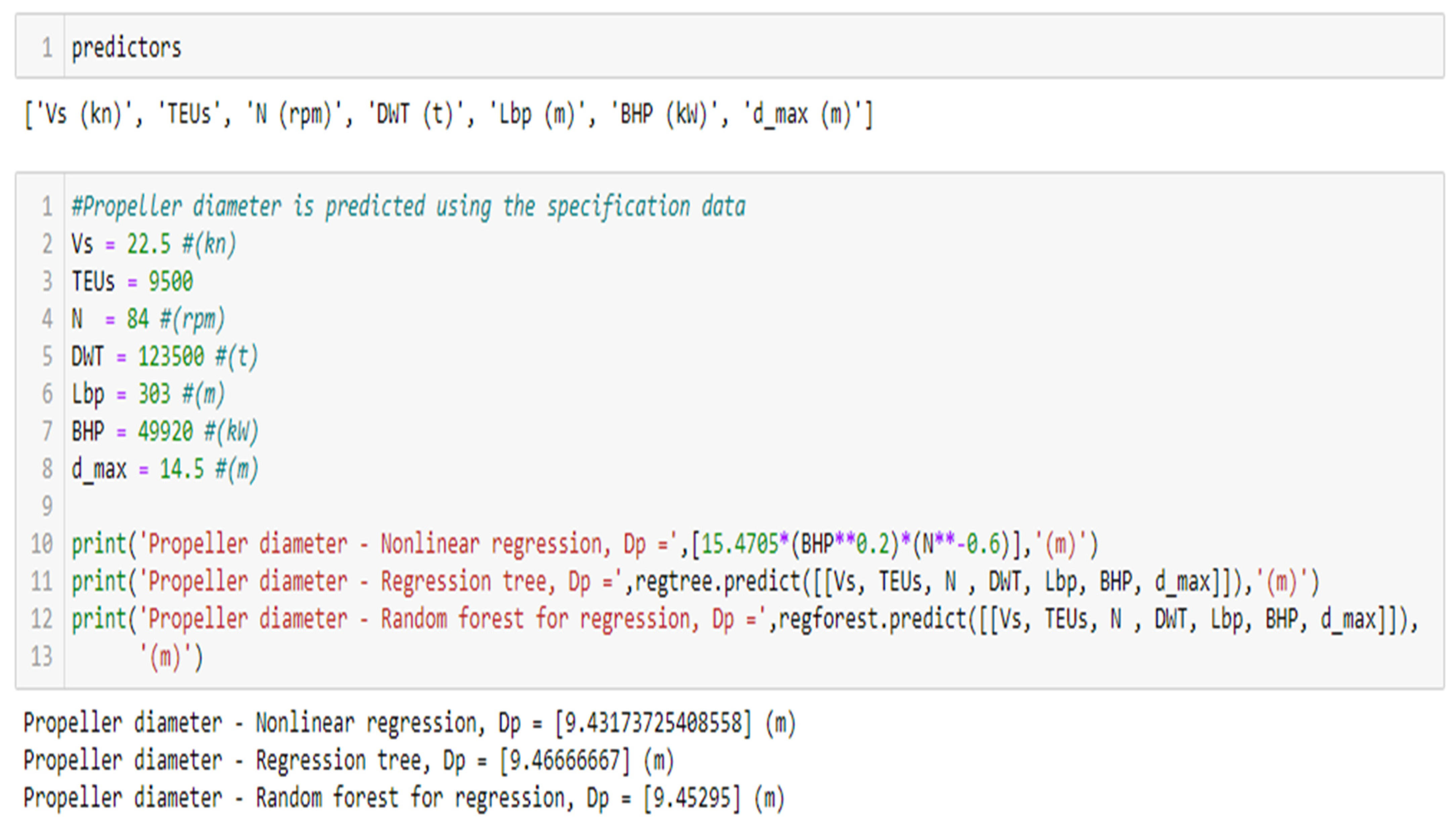
5. Prediction in the Propeller Diameter
Since the steps to follow are the same as in the previous section, the details of the procedure will not be entered again and only the results obtained will be discussed.
5.1. Estimation of Propeller Diameter before Analysis
For an estimation (prior to the analyses) of the propeller diameter, we used the formula provided by [
19], pp. 602–603.
To use this formula, it is enough to know the brake power and the propeller revolutions per minute.
where
Therefore, it is possible to calculate the propeller diameter in meters
(m) with the following data:
5.2. Definition of the Problem
The target variable is the propeller diameter, Dp.
For the study to be conducted, the propeller diameter,
Dp, will be considered as a function of:
where
(kW): Brake power.
(rpm): Propeller revolutions.
(kn): Ship service speed.
(tons): Deadweight.
: Number of containers (twenty equivalent units).
(m): Length between perpendiculars.
(m): Scantling draught
5.3. Elaboration of the Model with Machine Learning
The machine learning algorithms to be used are the same as for
Section 4.5 of this document.
5.3.1. Linear/Nonlinear Regression
On this occasion, only a regression that coincides dimensionally with the formula provided by [
19], pp. 602–603, for which
Table 3 is detailed, is used.
The result of the model is:
5.3.2. Regression Tree
The propeller diameter has already been studied and it is known that it is not a linear expression.
A regression tree can be another useful algorithm to predict the propeller diameter that would best fit the ship’s specifications. In addition, it has the advantage over regression that it is not necessary to predefine with a function how the variables are related.
With the same input and output variables, a regression tree was constructed, see the result in
Figure 14.
It is possible to enlarge the tree a little more by varying the hyperparameters, but care must be taken not to overfit the model.
5.3.3. Random Forest for Regression
Likewise, with the same input and output variables, a random forest for regression (composed of 1000 trees) was constructed. Remember that the rest of the hyperparameters vary randomly.
5.4. Goodness of Fit of the Models
Once again, the error is quantified following the
fold cross-validation technique that was explained in
Section 4.6.
See in
Figure 12 the errors committed in the prediction of the propeller diameter,
.
5.5. Estimation of Propeller Diameter after Analysis
According to Equation (14), provided by [
19], pp. 602–603 (applied in
Section 5.2), one has:
According to nonlinear regression using Equation (16):
According to the regression tree:
According to the random forest for regression:
The best predictive algorithms are random forest for regression and nonlinear regression, as it is stated in
Figure 15. Both can be considered good. Therefore, one option is to choose the average value of the diameter predictions for both algorithms.
6. Classification of Materials Used in the Propulsive System
When devising a system, a crucial task involves selecting the appropriate materials and considering a balance between the demanded mechanical behavior and material cost. Opting for a material that best aligns with performance needs is pivotal. In this regard, machine learning techniques can be employed to achieve classifications via clustering. This entails organizing a database comprised of materials for maritime usage, wherein materials with similarities are grouped while those with greater disparities are separated. The parameter guiding this distinction is the distance among data points. This approach offers a substantial advantage as it permits consideration of which material closely matches the imposed requirements. This algorithm could be directly integrated with an optimization problem.
For the purpose of this study, the problem will be streamlined by focusing solely on the main propulsion system.
Before delving further into the application of these algorithms, it is prudent to have a preliminary understanding of the materials used in propulsion systems.
We will start with the shaft. The shaft is primarily affected by corrosion, fatigue, and fretting corrosion. Coatings are employed due to the highly corrosive environment, although they remain vulnerable at the junctures between the metal components and coatings. Enhanced frictional fatigue of the tail shaft can be achieved by using a cold-rolled shaft surface; while this may not entirely prevent crack formation, it does impede their propagation [
20], p. 938.
Weldability is another vital aspect, as cracks stemming from corrosion fatigue can be rectified through grinding followed by the application of filler material through welding, thereby extending the shaft’s lifespan.
Commonly used materials for merchant ship shaft lines include high-strength steels which boast high carbon content, although their mechanical properties can diminish due to the corrosive environment. High-strength steel is employed for merchant ships with substantial power, such as the container ship project covered in this document.
Additional materials used encompass nickel–copper alloys (MONEL), precipitation-hardened stainless steels, manganese bronzes ( brasses), and more.
Now, turning to the propeller. When selecting propeller materials, the primary aim revolves around meeting the following properties:
Copper-based alloys have gained widespread use for marine propellers. These alloys offer sound mechanical properties and enhanced resistance to biofouling due to copper’s biocidal properties. Over the years, the trend has shifted toward employing high-strength nickel–aluminum bronzes and manganese–nickel–aluminum bronzes [
20], p. 938.
In certain specialized applications, materials like 12%
stainless steels, austenitic stainless steels, or titanium alloys may be used (though titanium comes with high mechanical performance but a corresponding high cost) [
20], p. 938.
6.1. Preparation of the Database
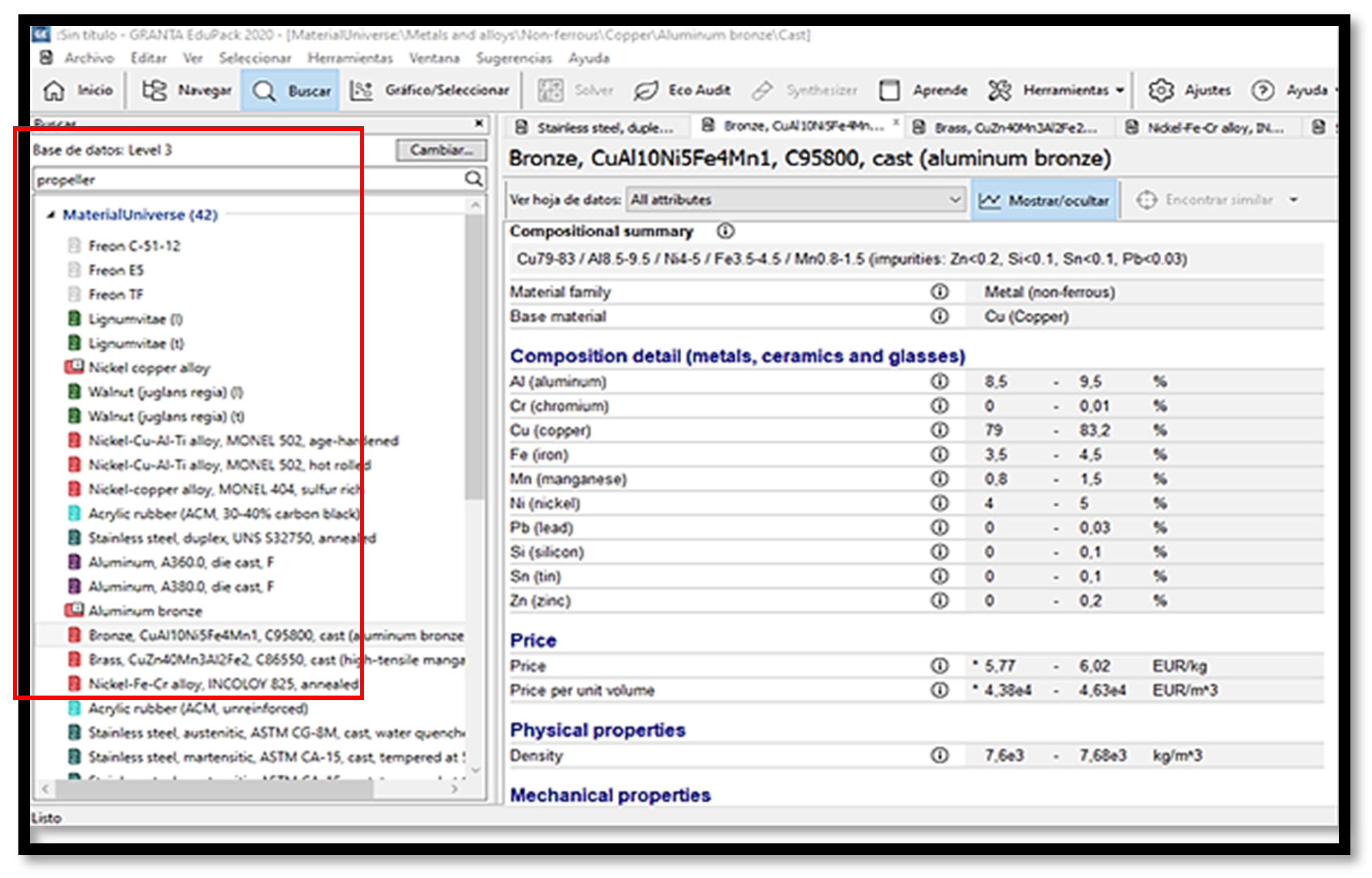
A database extracted from GRANTA EduPack 2020
®,
Figure 16, is elaborated from the Level 3 database, which is a very extensive and detailed database of materials. In this database, the materials used in propulsion systems have been filtered from the entry: propeller.
The collected variables encompass the mechanical properties of materials, price, corrosion resistance, durability in diverse environments, footprint for production and recycling, weldability, and castability properties, and more.
6.2. Elaboration of the Model with Machine Learning
The material selection process is divided into two distinct stages, each serving a unique purpose.
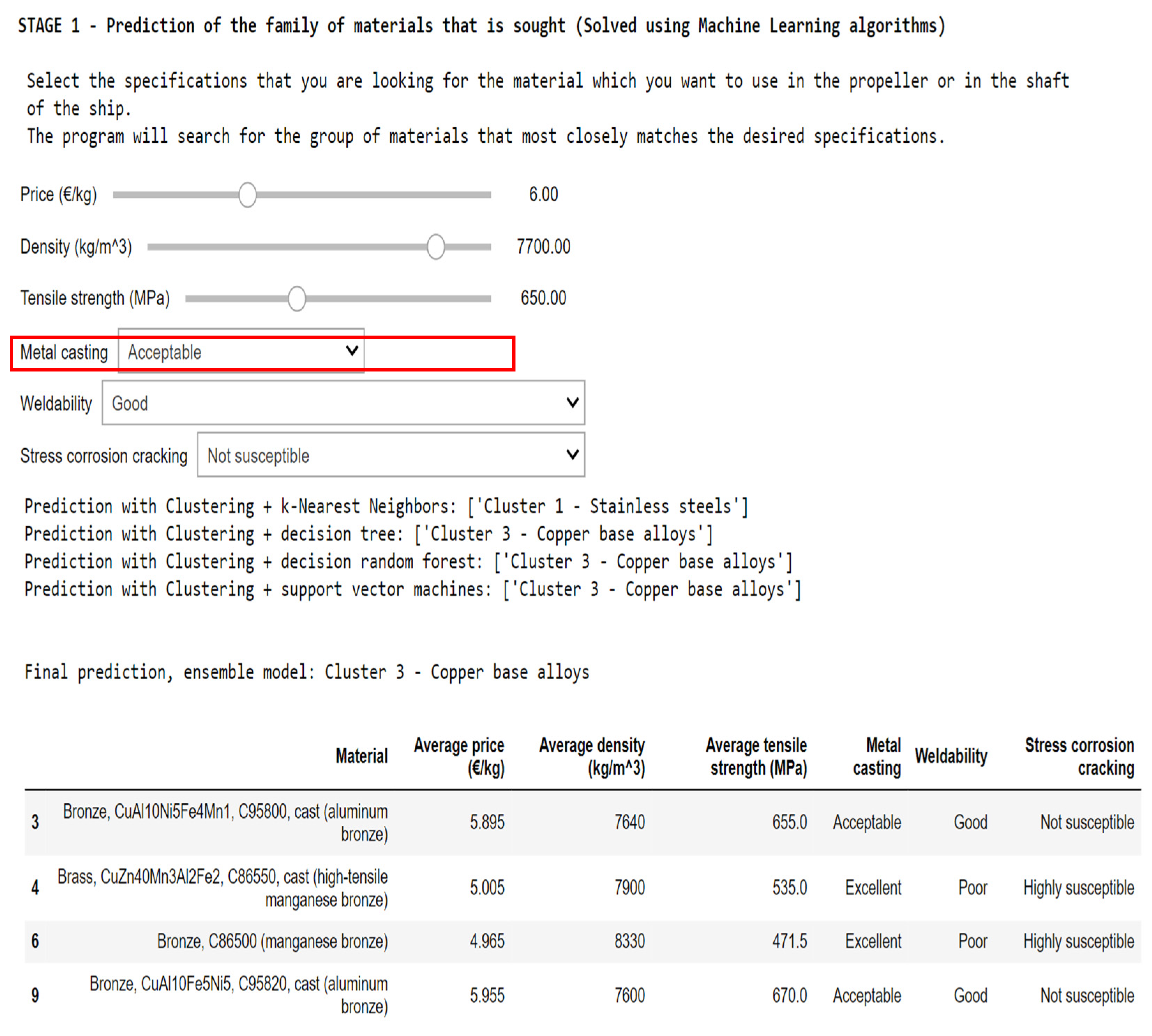
In the first stage, machine learning algorithms come into play. This begins with clustering, which sorts the database data. Subsequently, these clustered data points are utilized as inputs for various supervised algorithms, each designed to predict a categorical variable. Refer to
Figure 8 for guidance on choosing the appropriate algorithms based on the output variable types. The categorical output variable in question corresponds to the cluster formed through the initial clustering process. Following the class prediction, the algorithms are aggregated, combining their predictions via voting, as elucidated later in
Section 6.2. This initial stage aims to filter the materials that most closely align with desired specifications. Here, “assembly” refers to utilizing the output from one algorithm as input for another.
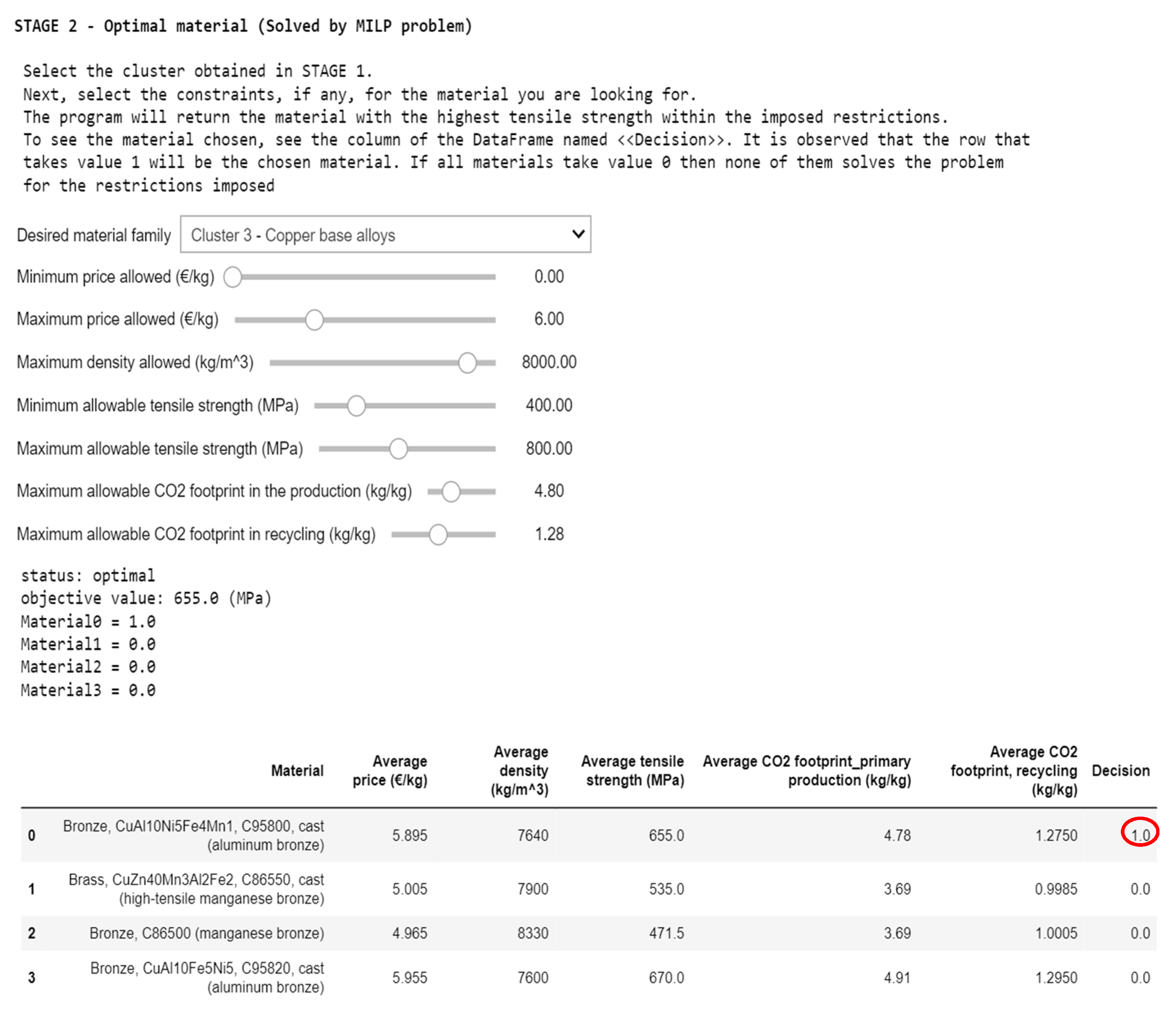
Moving to the second stage, an optimization process (see
Figure 17) is undertaken to identify the material boasting the highest tensile strength from the subset of materials filtered during the first stage. This selection must adhere to a set of constraints, ultimately resulting in the identification of a single material.
The first stage commences with the application of an unsupervised algorithm to structure the data. Employing an agglomerative hierarchical clustering technique and examining the resultant dendrogram, one can observe the grouping that the algorithm determines most suitable. This takes into account the similarities and differences among data attributes, essentially analyzing material properties to facilitate data grouping and segmentation.
Figure 18 illustrates the clustering outcome, showcasing the grouping of materials based on their similarity levels as indicated by the Euclidean distances among data points along the ordinate axis.
The algorithm’s classification proves coherent, effectively grouping materials within the same family to which they belong. In total, five clusters were identified.
Having grouped the data, we proceed to apply the supervised algorithms which serve to predict.
For the supervised algorithms, only six input variables ( will be used (of which three are numerical variables and the other three are categorical variables). The output is a categorical variable .
The input variables () for the material are the price (EUR/kg), density , tensile strength (MPa), properties for casting, properties for welding, and resistance properties against stress corrosion cracking.
The output variable () is the cluster to which the material would belong based on the desired specifications.
To confirm the models, a cross-validation is performed (with
equal to ten iterations). The procedure is the same as that calculated in previous sections, it is randomly split into a training set and a test set for each iteration. With the training set, the model is elaborated, and with the test set, the efficiency of the model is measured; the difference is that now what is going to be measured is the accuracy in each iteration for the test set.
This technique will be used with every one of the independent models obtained from the supervised algorithms and the accuracy of assembling the models will also be quantified, which basically consists of an absolute majority vote.
This vote is a soft vote. This means that in the hypothetical case of a tie vote, the probability of occurrence of the class predicted by each model will be considered. The one with the highest probability will be the class selected in the final prediction of STAGE I of the program.
Figure 19 shows a slight improvement when assembling the models since a higher accuracy value has been obtained.
6.3. Assembly with MILP Optimization Problem
After completing the first stage, which aims to filter the family of materials that most closely resembles the desired specifications, the second stage in the selection of the material begins, which consists of applying a linear optimization problem.
Finally, to obtain a material that provides the best performance within the family of materials, the results obtained are assembled with an optimization problem.
The goal of the optimization problem is to find the highest tensile strength.
Based on the results obtained, only the materials that belong to the family of copper-based alloys have been filtered.
The Mixed Integer Linear Programming (MILP) optimization problem is defined.
- ○
Decision variables (unknown to the problem):
For = 0, 1, …, n − 1
is a binary variable (it is 0 if the material is not chosen and 1 if it is the chosen material).
Where
- ○
: The subscript that identifies the material.
- ○
: The total number of materials inside the cluster obtained from machine learning.
- ○
Parameters (known to the problem):
Where
- ○
: The subscript that identifies the material. Each parameter is defined by the subscript since the parameters are known within the dataset.
- ○
Objective function: max .
- ○
Restrictions: Subject to
- ○
: Minimum price allowed (EUR/kg);
- ○
: Maximum price allowed (EUR /kg);
- ○
: Maximum density allowed (EUR /kg);
- ○
: Minimum tensile strength allowed (MPa);
- ○
: Maximum tensile strength allowed (MPa);
- ○
: Maximum footprint in the production allowed (kg/kg);
- ○
: Maximum footprint in the recycling allowed (kg/kg).
The problem may or may not have a solution. The more restrictive the problem, the less chance there is of finding a solution.
The problem has been solved with the
Optlang library [
22]. In ANNEX VI, it has been further solved with the
PuLP library [
23]. The same results were obtained for both libraries.
6.4. Interactive Program
Obviously, implementing all these algorithms requires an investment in time when extracting the data, cleaning it, and applying the models. However, it is always sought to automate the code so that it is as comfortable as possible when it comes back to future projects.
In the Jupyter
® V7.0.3 notebook that is attached to this work, all the code has been grouped in a single cell and an interactive program has been developed. To use the program, it is only necessary to run the three code cells, and the screen shown in
Figure 20 and
Figure 21 will appear.
It is easy to use. Only input variables and the restrictions to be imposed are introduced.
During the initial stage, the desired specifications are designated by manipulating the control bars and selecting options from choice boxes. Following this, the first stage yields a cluster prediction along with a corresponding table listing the materials affiliated with that cluster. Once the initial stage concludes, the program advances to the second stage.
In the second stage, the cluster derived from the ultimate prediction of the first stage is chosen, alongside the specifications for the MILP optimization problem.
7. Discussion: Deep Learning and Future Lines of Study
The concept of deep learning is often regarded as an advancement over machine learning. In this scenario, the level of interaction between users and machines is minimized. In the realm of deep learning, the focus revolves around crafting the architecture of a neural network that meticulously processes the data.
Within the domain of deep learning, users play a pivotal role in defining hyperparameters. These parameters encompass crucial aspects such as the count of neuron layers, where a minimum of two layers—a designated input layer and a corresponding output layer—is mandatory.
Notably, intermediate hidden layers frequently intercede between the input and output layers, significantly enhancing the precision of prediction and classification outcomes.
Moreover, the hyperparameters encompass determining the number of neurons per layer.
This entails having a corresponding number of neurons in the input layer as there are input variables. Similarly, the number of neurons in the output layer aligns with the target variable’s count, underlining the comprehensive nature of the parameter configuration in deep learning.
Neurons within a neural network are interconnected, with each connection being assigned a specific weight.
As illustrated in
Figure 22, a neuron fundamentally operates by aggregating the weighted summation of its inputs and associated weights. Subsequently, an activation function, functioning as a filter, is applied. This function serves to activate neurons that demonstrate favorable outcomes.
Figure 23 showcases some commonly employed activation functions.
Activated neurons generate outputs, contributing to the iterative training of the neural network. During the initial iteration, the network’s predictions may be inaccurate, as learning has not yet transpired. Here, the pivotal role of backpropagation emerges. Neurons predict layer by layer, culminating in the output layer. After prediction, the algorithm assesses errors by traversing the network backward. Correct predictions reinforce the weights linked to neuronal connections, intensifying the network’s intelligence. Consequently, an increased number of iterations enhances weight reinforcement, resulting in heightened neural network competence.
For neural network construction in Python3®, TensorFlow and Keras libraries are commonly employed. These libraries, the most widely used, facilitate the development of neural networks. A distinctive advantage of deep learning over machine learning lies in its adeptness at handling unstructured data more efficiently. While this study utilizes structured, tabulated data, deep learning is particularly adept at handling unstructured data, such as images, videos, audio, and text.
The forthcoming research trajectory envisioned for this study involves predicting ship propeller cavitation wear rates using images obtained during periodic inspections. This entails employing intricate neural network architectures and gathering a database of propeller images accompanied by wear rate study outcomes. If the images are in color, a conversion to black and white will be undertaken, as color intensity values per pixel are more interpretable with a neural network. Refer to
Figure 24 for an example of the images constituting the database.
Subsequent phases involve formulating neural network architectures based on the acquired knowledge and training them using the image database as input variables, with the cavitation wear rate as the output variable. The neural network’s potential lies in utilizing propeller images to detect wear due to air bubble implosion from cavitation and assessing the resultant cavity shape. Linking each image to a parameter quantifying corrosion-induced wear—such as material loss—enables the neural network to predict based on insights gleaned from the image database. Following training, the neural network can swiftly assess the ship propeller’s condition during routine inspections by predicting future images captured during such evaluations.
8. Findings and Conclusions
The investigation yielded noteworthy findings regarding the performance of each machine-learning algorithm in predicting braking power and propeller diameter. The root mean square error (RMSE) values for these predictions were consistently lower than those derived from J. Mau’s braking power calculation formula and the propeller diameter formula [
19], p. 602. These improved predictions effectively address the initial query about the quality of the machine learning predictions posed at the study’s outset.
Furthermore, it is worth noting that there exists a significant correlation among predictor variables. This observation is not surprising given the interconnectedness of variables related to cargo capacity and ship size. This high correlation substantiates the validity of the predictive model.
The efficacy of clustering was demonstrated and particularly evident in its application to material classification. The algorithm was adept at structuring data and grouping elements solely based on the information they offered. This significance amplifies when dealing with data whose underlying behavior is less apparent.
Ensemble models, constructed through the amalgamation of algorithms, displayed an accuracy of 93.33%. This accuracy surpasses that of individual algorithms, highlighting the enhanced robustness attained through algorithm assembly.
The obtained results are gratifying and signify a marked improvement in prediction accuracy. The maritime industry stands to benefit from the diverse applications of these algorithms. While this study concentrated on specific machine learning algorithms, there remain unexplored avenues, and the realm of deep learning warrants further exploration, especially concerning neural networks’ capacity to predict propeller cavitation wear rates using images.
In line with this investigation’s outcomes, it is evident that the developed models possess the ability to scrutinize vast volumes of intricate data, thereby producing more precise outcomes.


