Article

Numerical Investigation of Global Ice Loads of Maneuvering Captive Motion in Ice Floe Fields

1
Key Laboratory of High-Performance Ship Technology, Wuhan University of Technology, Ministry of Education, Wuhan 430063, China
2
School of Naval Architecture, Ocean and Energy Power Engineering, Wuhan University of Technology, Wuhan 430063, China
3
China Ship Development and Design Center, Wuhan 430064, China
*
Authors to whom correspondence should be addressed.
J. Mar. Sci. Eng. 2023, 11(9), 1778; https://doi.org/10.3390/jmse11091778
Submission received: 25 July 2023 / Revised: 31 August 2023 / Accepted: 1 September 2023 / Published: 11 September 2023
(This article belongs to the Special Issue Design of Marine Structures against Ice Actions)

Abstract

:
During escort and convoy operations, icebreakers are often required to maneuver to open up channels or adjust routes due to the prevalence of ice floe conditions in Arctic routes. This study aimed to investigate the global ice load characteristics of the maneuvering captive motions, including constant turning motion, pure yaw motion, and pure sway motion, of the icebreaker Xue Long, using a combination of the discrete element method (DEM) and drag model. First, the method was verified using simulating Araon model tests from the Korea Institute of Ocean Science and Technology (KIOST). In addition, the maneuvering captive motions of the Xue Long model were simulated at varying turning radii, drift angles, and sway and yaw periods, which are typical but currently poorly studied maneuvering motions. Overall, the results of the study showed that the method is able to reproduce the coupling effect of the ship–ice–water system by considering ship–ice interaction and ice resistance, where the mean deviation and maximum deviation of ice resistance are 9.45% and 13.3%, respectively. The influences of the turning radius, drift angle, and sway and yaw period on the ice resistance and transverse force characteristics were studied and analyzed via ship–ice interactions. The present study provides a prediction tool for the assessment of ship maneuvering performance to assist the hull line development and model testing of icebreakers.

1. Introduction

In recent years, the amount of freight traffic through Arctic routes has risen, and there is still great potential for this to rise in the future [1,2]. As the basic piece of equipment for navigation in ice fields, an icebreaker’s maneuverability is key to ensuring the safety of fleet navigation [3]. The prediction of ship maneuvering performance in ice fields is different from that in open water, and the complexity of ship–ice–water interaction poses a challenge to the global ice load prediction of ships.
Ice floe fields are one of the most common types of broken ice along Arctic routes, and ice floes collectively cover about 5% of the Arctic Ocean. Their coverage is about 30% along the northern sea route (NSR), and icebreakers break the level ice sheet and produce additional broken pieces along the NSR channel [4]. Since the 1960s, researchers have proposed parameters to describe ice floe fields through the mathematical models established when studying the dynamic process of sea ice, such as its concentration, thickness, and average size [5]. At present, the global ice load calculation methods for ships can be divided into three categories: theoretical–empirical formula, model–real-ship test, and numerical simulation.
In the early stage, the interaction of ice floes and ships in ice resistance and mooring problems was studied by combining model tests, full-scale measurements, and theoretical–empirical formulas. The former Soviet Union conducted a lot of research on the navigation performance of ships in ice floe conditions by using model tests and full-scale ship test trials to arrive at some empirical formulas, for example, the 1959 Bronnikov resistance formula [6] and the Buzuev and Ryvlin resistance formula [7]. In 1969, Kashteljan [8] divided total ice resistance into four parts: inertia term, dissipation term, ice limitation term, and water resistance term. In 1999, Nozawa extended this to include the ice load calculation of floating structures with complex shapes [9]. During the 1970s and 1980s, the US Army Corps of Engineers Cold Regions Research and Engineering Laboratory (CRREL) conducted a large amount of experimental research on USCGC ships and put forward an empirical formula for ship resistance under ice floe conditions [10]. In 1996 and 1998, Keinonen and Robbins developed a method for calculating resistance by using formulas in ice and proposed the concept of “equivalent” ice thickness [11,12]. In 1989, Aboulazm considered the application of early empirical formulas to different ship types and proposed two analysis models to calculate the resistance: micro and macro models. The micro model represents the case of medium-speed ships with a water surface distribution density of less than 50%, and ice is a discrete body flowing toward the hull. The macro model represents the case of ice concentrations greater than 50%; in this case, the ice field is treated as a continuum [13]. In 2009, Spencer and Molyneux constructed a resistance formula based on model tests and applied it to various ship mooring problems [14].
With the development of numerical methods and the enhancement of computational technology, numerical methods have been widely applied in studies on ship performance in ice. In particular, DEM is frequently applied due to the discrete distribution characteristics of ice floes. In 1992, Hopkins introduced DEM into the interaction between ships and ice floes [15]. In 1994, Løset used the two-dimensional disc discrete element method to study the interactions between ice floes [16,17]. In 1999, Hansen and Løset extended this method to calculate the interaction between ice and ships [18].
Since then, DEM has been widely used to assess the interaction of ice floes and ships. Among them, Japan’s Konno has conducted a large amount of research in this area, using the non-smooth discrete element method with discs and discrete spheres to solve the ice loads on ships sailing in ice floe fields [19,20]. The Norwegian University of Science and Technology developed the commercial software SIBIS, which is also based on the non-smooth 3D formulation of DEM [21,22]. In 2015, Metrikin et al. used SIBIS to calculate the performance of a floating drillship operating under intact and managed sea ice conditions [23,24]. Other representative studies include the research conducted by Lau et al. [25,26] and Liu et al. [27,28] in Canada. DEM has also been used to calculate ship–ice interaction forces by using the commercial software DECICE.
In terms of maneuverability in ice, Lau [29] and Lau and Simoes [30] in 2006, Zhan and Agar in 2010 [31], and Zhan and Molyneux in 2012 [32] used DECICE to calculate ship–ice interaction force and predict a ship’s maneuverability in level ice. In Zhan et al.’s study [31,32], the MMG (Maneuvering Modeling Group) standard method for ship maneuvering predictions, introduced by Yasukawa and Yoshimura [33], was used to solve the ship-maneuvering motion equation and predict the maneuvering motion of a ship in pack ice. From 2012 to 2016, Daley et al. used graphics processor technology to significantly improve the computational efficiency of the DEM method for ships in ice floe fields, subsequently making this method more applicable [34,35]. In addition, some partial empirical numerical models have been extensively developed and applied to the study of ship-maneuvering performance in level ice. In 2009, based on the analytical approach and its numerical implementation, Liu [28] first proposed and established a fully mathematical numerical model that can develop a real-time three-degrees-of-freedom (DOF) simulation of an arbitrary ship‘s maneuvering motion. In 2010, researchers from the Norwegian University of Science and Technology, Rsika and SuBiao et al. [36,37], constructed a partial empirical numerical model that considered local ship–ice interaction, the overall performance of the icebreaker, and the statistical characteristics of the local ice load of the hull, and they used it to solve the 3DOF maneuvering motion of the icebreaker. In 2014, TanXiang [38,39] extended the maneuvering model of Su to 6DOF, improved the relationship between the local contact area and pressure of a ship and ice to understand the dynamic bending failure of sea ice, and adopted computational geometry to establish 3D hull geometry in the model. A partial empirical numerical model was also constructed to solve the 6DOF maneuvering motion of a fully coupled 6DOF ship and its local and global ice loads in the time domain.
As two main ice conditions, the most intuitive difference between level ice and broken ice lies in the discontinuity of broken ice in space. There are many kinds of broken ice, such as brash ice, ice ridge, ice floes, and sliding ice pieces, under an advancing ship during a model-scale test [40]. In an ice floe field, the shape, distribution, and size of ice floes are uncertain and random, and large-scale ice floes may fracture under the action of waves. These characteristics make the study of maneuvering performance in an ice floe field more complicated than that of level ice; however, it is necessary and important to study maneuvering performance in an ice floe filed.
In summary, many studies have examined the ship–ice interaction processes in ice floe fields; however, compared with studies which focus on level ice conditions, there are much fewer studies on ice floes. Furthermore, the existing research into ice loads is mainly based on ice resistance, and studies on the ice load characteristics within ship maneuvering motions are rare. Due to this current research status, this paper focuses on the simulation of some typical maneuvering motions within ice floe conditions and studies ice load characteristics, including constant turning, pure yaw, and pure sway motions.
In this study, ice floes were constructed using the particle cluster of EDEM software [41]. EDEM is a unique and efficient method for generating cluster particles, making it suitable for floe ice modeling in floe fields, whilst also providing improved visualization and data tracking and analysis functions. Considering the buoyancy and drag force on ice floe, a numerical simulation of the maneuvering captive motions of the Xue Long icebreaker was carried out in the regular shape and uniformly distributed ice floe field. The DEM numerical model was validated using the direct towing test data of KIOST’s Araon icebreaker model [4]. Subsequently, this study carried out a numerical simulation of constant turning, pure yaw, and pure swag motions and studied the influence of the turning radius, drift angle, and swaying period.

2. Numerical Model of Ship Motion in Ice Floe Field

2.1. The Governing Equation of DEM

In DEM, the motion of particles is based on Newton’s second law and can be decomposed into translation and rotation, which are determined by the normal force, shear force, and torque acting on the particle unit as a result of interparticle interactions.
The translation and momentum conservation equation of ice floe, i , is as follows:
m i d u i d t = j F i j + F f l u i d + F b g
The angular momentum conservation equation of ice floe, i , is as follows:
I i d ω i d t = j T i j
where m i , u i , and ω i , respectively, represent the mass, translational, and angular velocities of the ice-floe discrete elements, i ; F i j is the collision force between element i and j and other non-contact forces acting on the particle; F f l u i d is the force of fluid on particle i ; F b g is the body force (due to gravity) of particle i ; I i is the rotational inertia of particle i ; and T i j is the contact moment, which represents the torque generated by the contact force on the particle.

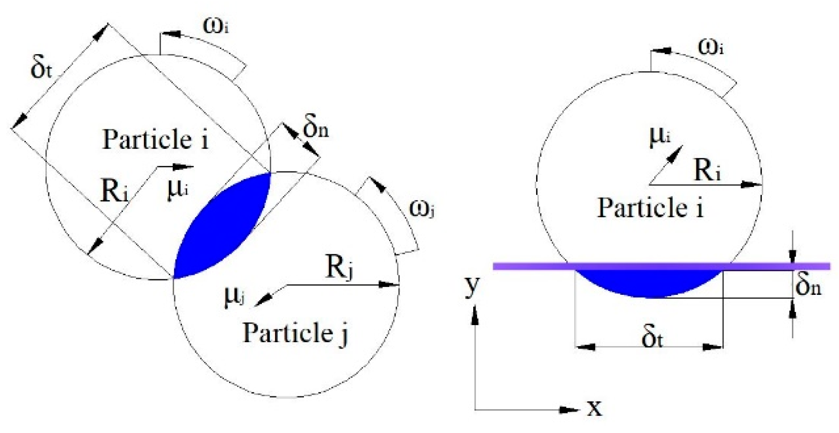
2.2. Interactions of Floe–Floe and Hull–Floe

The numerical model of ship motion in ice floe fields includes floe–floe and floe–ship interactions. This paper mainly studies the influence of ship-maneuvering motion parameters on ice loads under small-scale ice floes. Generally, an ice floe in the equivalent range of 20~100 m is considered small-scale floating ice [42], but in these simulations, the real scale width of ice floes is about 2.2~6 m and 0.12~0.26 B. At this scale, the breaking phenomenon of ice floes under general ship motion is very slight and can be neglected. At this time, the ice load is mainly caused by a collision with the hull and the friction generated when ice floes slide along the hull.
Ice breaking and refreezing are not considered comprehensively in these simulations. The assumption of ice floe as a rigid body can reduce the calculation cost under the premise of ensuring accuracy and is conducive to carrying out a series of numerical simulations to study the variation law and mechanism of the ice load of ship maneuvering in floating ice. Moreover, the ice floe–ice floe and hull–ice floe contacts are assumed to be elastic. The Hertz–Mindlin contact model was adopted, in which the contact forces are calculated, as shown in Figure 1. The contact forces can be divided into normal and tangential forces, and both contain damping components.
The normal contact force is as follows:
F n = 4 3 E ( R ) 1 / 2 δ n 3 / 2
where δ n is normal overlap; and the equivalent Young’s Modulus, E , and the equivalent radius, R , are defined as follows:
1 E * = 1 - u i 2 E i + 1 - u j 2 E j 1 R * = 1 R i + 1 R j
The normal damping force is as follows:
F n d = 2 5 6 β S n m u n v e l
where u n v e l is the normal component of the relative velocity between the interacting elements, and m is the equivalent mass.
Moreover, m , β , and S n (the normal stiffness at contact) are given by the following:
m = m i m j m i   +   m j β = l n e l n 2 e   +   π 2 S n = 2 E R δ n
The tangential contact force is calculated as follows:
F t = S t δ t
where δ t is the tangential overlap; S t is the tangential stiffness at contact, S t = 8 G R δ n ; and G is the equivalent shear modulus of the interacting elements.
The tangential contact force is limited by Coulomb friction, u s F n , where u s is the coefficient of sliding friction.
The tangential damping forces are represented by the following:
F t d = 2 5 6 β S t m u t v e l
where u t v e l is the relative tangential velocity.
In contact, the torque depends on the relative rotational velocity of two particles, as follows:
T i = u r F n R i ω i
where u r is the coefficient of rolling friction, and ω i is the unit angular velocity vector of the object at the contact point.
For normal and transverse floe–hull interaction forces, the formulas stay the same, but the radius and mass of the hull are R s h i p = and m s h i p , respectively, so the equivalent radius is R = R f l o e , and the equivalent mass is m = m f l o e .

2.3. Interaction of Water–Ice Floe

The interaction of water with ice floes mainly includes the buoyancy force and drag force, which are shown in Figure 2. The infinitesimal element method (IEM) was used to calculate these forces. The IEM is used to treat the ice floe, which is composed of clusters of particles, as a regular cuboid, and then the cuboid is uniformly discretized into several infinitesimal elements, as shown in Figure 3a. Next, the forces of each element are calculated by fixing the water level, using the Archimedes’s and drag formula. The forces of the elements are finally converted to the center of the mass of the ice floe, and then the buoyancy and drag force of the entire ice floe are calculated. Part a in Figure 3 details a schematic diagram of the discretization process.
The buoyancy force acting on the element (taking element m as an example, which is completely submerged in water, and the external area is subjected to fluid action) and the ice floe is as follows:
F b m = ρ f g V m
F b u o y = F b m z
The torque acting on the element and ice floe is as follows:
T b u o y = F b m z × L
where ρ f is the density of water, g is the acceleration of gravity, V m is the volume of m element immersed in water, z is the unit vector of the Z-axis, and L is the vector length of the mass center of the ice floe and m element.
The drag force acting on the m element and the ice floe is as follows:
F d m = k R e c A ρ f v f v p v f v p
F d r a g = F d m
T d r a g = F d m × L
where R e is the Reynolds number of the ice floe; A is the external area of the m element subjected to fluid action; v f and v p are the velocity of water and m element, respectively; and k and c are, respectively, the coefficient of drag and the coefficient of the Reynolds number. Both c = 0.012 and k = 0.6267 were obtained via numerical simulation, using FLUENT.

2.4. DEM Ice Floe Fields

An ice floe is composed of many evenly arranged spherical particles, of which there are 2–3 layers of particles in the thickness direction. In the tests of the Araon, the shape of the ice floe is a cuboid [4], so the geometric shape of the ice floes used in these simulations is also a cuboid, and the particles are evenly arranged. An ice floe particle and the model of the ice floe field are shown in Figure 3.

2.5. Validation

Direct towing tests of the Araon were carried out at the KIOST’s ice tank. The towing speeds were 0.238, 0.357, and 0.476 m/s; the sizes of the ice floe were 0.25 × 0.25 × 0.04 m and 0.12 × 0.12 × 0.04 m; and the concentration was 6/10. The cutting of the parental ice sheet and the resulting ice floe field for the tests are shown in Figure 4. The lines of the Araon are outlined in Figure 5 [4,43]. The main parameters of the Araon are detailed in Table 1. To avoid the influence of floe distribution on the numerical simulation results, ice floes in all simulations are uniformly distributed, as shown in Figure 3b.
Figure 6 shows the ice resistance curves of the Araon. Figure 7 shows a comparison between DEM simulation values and KIOST test values, which are in good agreement. The general trend of the ice resistance value is consistent with the increase in ship speed, and more violent collisions of ship–ice are one of the reasons for the increase in the ice resistance value. The main cause of the ice load acting on the ship is the process of the hull displacing the ice floes and forming the channel. An increase in speed causes the hull to travel more distance in the same amount of time, which, in turn, displaces more ice floes, which intensifies the collision between the hull and the ice floes and consumes more energy, resulting in an increase in resistance. The simulation values are within 15% error bands, of which the maximum error is 13.33% and the average absolute error is 9.45%. The errors may be due to the distribution of ice floe and the secondary breaking of ice floe during the tests.

3. Numerical Simulation of Constant Turning Motions: Turning Radius and Drift Angle

The rotation performance of the ship in a pack ice field is very important compared with that in open water, and the turning radius and drift angle are key parameters in the turning maneuvers. In this study, the model of the Xue Long icebreaker was used, and the constant counterclockwise turning motion of the Xue Long was simulated. The speed is 0.563 m/s; the ice concentration is 60%; and the floe thickness and side length are 0.0267 m and 0.2 m, respectively. Different drift angles and turning radii were selected to study their influence on ice loads. The main parameters in the numerical simulation are shown in Table 2. The geometric model and main parameters of the Xue Long are shown in Figure 8 and Table 3. The computational domain consists of a rectangle and a quarter ring, as shown in Figure 9. Figure 9 also shows the coordinate system used in the simulations: O 0 X 0 Y 0 is the earth-fixed coordinate system, where the X 0 Y 0 plane coincides with the still-water surface. O XY is the fixed-body coordinate system with the origin, O , taken at the center of gravity of the ship, and the X -axis and Y -axis points, respectively, are toward the bow and port. The ice resistance is positive in the negative direction of the X-axis, and the transverse force is positive in the negative direction of the Y-axis. The drift and turning angle are also defined in Figure 9.

3.1. Analysis of the Steady Turning Motion

This section simulates the steady turning motion of the Xue Long at a 4 deg drift angle ( β = 4   deg ) and 2 L turning radius (R = 2 L), where L is L p p in Table 3. The numerical results of the steady turning motion are analyzed from the two aspects of the ice loads’ time history curves and the interaction between ice floe and the Xue Long. The motion begins with an oblique drifting motion at t = 0 s, and the hull enters the ice floe field. At t = 10 s, the hull completely enters the ice floe field, and the hull begins to carry out the steady turning motion; the numerical simulation is completed at about t = 40 s.
Figure 10 and Figure 11 detail the time history curves of ice resistance and transverse force and the changes in total energy between ice floe and ship at 5 s, 10 s, 25 s, 30 s, 35 s, and 40 s, respectively. It can be seen from Figure 10 and Figure 11 that ice resistance increases from 0 s to 5 s and no longer increases with time when most of the hull enters the ice floe field. After t = 10 s, the hull begins to carry out a constant radius motion; at this stage, the ice resistance increased slightly, but after about t = 20 s, the ice resistance no longer increased with time and fluctuated within a range. In the Y direction of the hull, the t = 0~10 s hull is in the transitory stage, and the transverse force fluctuates greatly. After t = 10 s, there were many ship–ice interactions on both sides of the hull. It can be seen in Figure 11 that the influence area of the port side on the ice floe field is significantly greater than that of the starboard side, so the transverse force points toward the starboard side. After t = 20 s, the transverse force no longer increases with time and fluctuates roughly in a range.

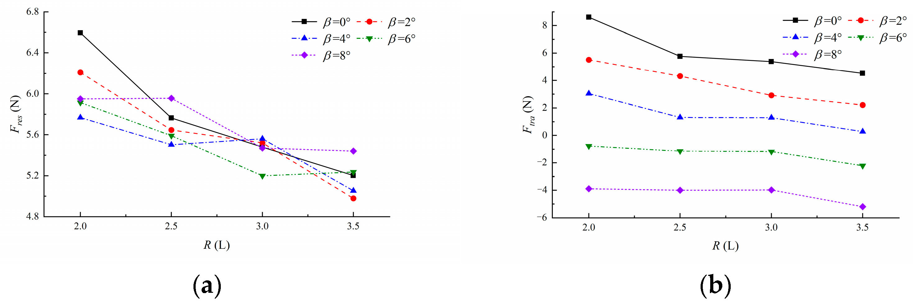
3.2. Analysis Influence of Varying Turning Radius

Figure 12 and Figure 13 are the box-plot diagrams of the ice resistance and transverse force for four turning radii (R = 2 L, 2.5 L, 3 L, and 3.5 L) and five drift angles (β = 0 deg, 2 deg, 4 deg, 6 deg, and 8 deg), respectively. It can be seen that with the increase in the turning radius, the ice resistance is always right-skew distributed, with the average and median values of ice resistance generally showing a downward trend, and the distribution of ice resistance in the range of 25~75% shows a narrowing trend. The skewness distribution is relative to the normal distribution and can be divided into right-skewed distribution and left-skewed distribution. When the mean is greater than the median, it is right-skew distributed; otherwise, it is left-skew distributed [44]. In addition, the average values, the median values, and the distribution of the transverse force show a slight trend to decrease.
Both Figure 14 and the slight decrease trend of the transverse force suggest that, with the increase in the turning radius, the degree of the ship–ice-floes’ interaction decreases on the whole. However, the interaction between the hull and ice floes slightly intensifies in some local reigns, such as the starboard side of the mid-ship and the port side of the mid-ship. The mid-ship starboard and ice floe appear to experience a contact collision phenomenon at R = 3.5 L. This is similar to the influence of the turning radius on the ice loads found in Liu’s [28] and Lau’s [45] discussion and conclusion. Liu found that increasing the turning radius in the ice layer reduces the ice load by reducing the ship–ice contact area through the use of model tests and numerical simulations. From a geometrical point of view, Lau investigated the effect of the stern shape on the turning process in level ice and found that a rounder stern shape and an increase in the turning radius can reduce the ice broken pressure at the stern, thereby reducing the ice load of the maneuvering motion.
Table 4 and Figure 15 show the average ice resistance and transverse force at different drift angles and turning radii, respectively. With the increase in the turning radius, the ice resistance and the transverse average show a downward trend, and the transverse force of the hull decreases. When the hull performs a counterclockwise constant radius motion, the contact collision between the ship’s port side and the ice floe is more serious than that of the ship’s starboard region. A small turning radius increases the possibility and area of contact between the stern and back shoulder and ice floes, which causes the position of the ship–ice interaction to move backward. Moreover, the midship and stern of the Xue Long have large slope angles. The combined action of the above points makes the ice load larger under a small turning radius.

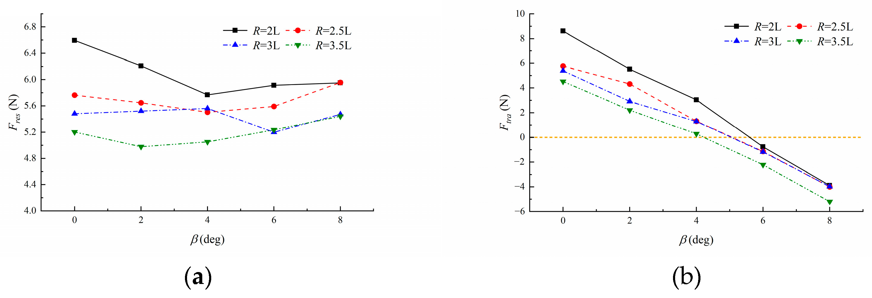
3.3. Analysis of the Influence of Drift Angle

Figure 16 shows the diagram of the turning motion with drift angles. Figure 17 and Figure 18 display the box-plot diagrams of ice resistance and transverse force under a constant radius motion with different drift angles under four turning radii. It can be seen that with the increase in the drift angle from 0 deg to 8 deg, the average values, the median values, and the distribution of ice resistance in the range of 25~75% have no obvious change law, and they all retain the characteristics of right-skewed distribution. However, the average and median values of the transverse force showed a downward trend, and the transverse force changed from a right-skewed distribution to left-skewed distribution.
With the increase in the drift angle, the interaction between the two sides of the mid-ship and the ice floe changes greatly. Figure 19 shows the change in the total energy at different drift angles at R = 2 L. The collision between the ship and the ice floe mainly concentrates on the port side and the bow, and there was almost no contact collision with ice floe on the mid-ship starboard side in β = 0   deg . With the increase in the drift angle, form Figure 19, a reasonable speculation can be made that the contact surface between the ice floe and mid-ship starboard side gradually increases, and it is expected that the influence range on the starboard side increases, while the influence range of the port side significantly decreases. When the drift angle increases to 6~8 deg, the port side of the mid-ship only collides with a small amount of ice floe, and a small open area is formed from the mid-ship port side to the stern. In other words, the interaction between the ice floe and the mid-ship starboard intensifies, while the mid-ship port weakens. Within this ebb and flow, the transverse force changes from pointing to starboard to pointing to port.
Figure 20 shows the curve of the average ice resistance and transverse force at different drift angles. When the drift angle increases from 0 deg to 8 deg, the average ice resistance has no obvious change trend, while the average transverse force decreases. When the drift angle is 4–6 degrees, the transverse force appears to be zero, and the direction also changes. At β = 6   deg and β = 8   deg , the average transverse forces become negative. In summary, the drift angle mainly affects the distribution of hull–ice collision events along both sides of the hull. When the hull performs a counterclockwise constant radius motion, the contact collision between the bow and shoulder of the port side and the ice floe is more serious than that of the starboard side. The increase in the drift angle increases the contact area between the starboard side and ice floe and decreases the contact area between the port side and ice floe, resulting in the force from ice floe on the starboard side being greater than that on the port side.

4. Numerical Simulations of Planar Motion Mechanism: Pure Yaw Motion and Pure Sway Motion

In this section, numerical simulations of the pure yaw and pure sway motion of the Xue Long are carried out to study the ice load characteristics and the influence of the period on the characteristics of the ice loads. Pure yaw, shown in Figure 21a, is a kind of motion in which the heading angle sinusoidally changes while the ship model advances at a constant speed, and the motion law of the ship is as outlined in Equation (15). Pure sway, shown in Figure 21b, is a motion in which the ship model advances at a constant speed and a sinusoidal transverse displacement is superimposed, and the motion law of the ship is as shown in Equation (16).
The side length and thickness of the ice floe are 0.2 m and 0.0267 m, respectively. The concentration of the ice floe field is 60%, the speed of the ship model is 0.563 m/s, and the heave and pitch of the ship model were restricted. Pure yaw and pure sway under three periods (T = 8 s, T = 12 s, and T = 16 s) are simulated and analyzed in terms of ice loads and ship–ice interaction.
The motion law of pure yaw is calculated as follows:
ψ = ψ m a x sin ( ω t ) r = ψ m a x ω cos ( ω t ) r ˙ = ψ m a x ω 2 sin ( ω t )
where ψ is the heading angle; and r and r ˙ are the yaw angular velocity and yaw angular acceleration, respectively.
The motion law of pure sway is calculated as follows:
y = y m a x sin ( ω t ) v = v m a x cos ( ω t ) ,   v m a x = y m a x ω v ˙ = y m a x ω 2 sin ( ω t ) ψ = 0
where y is the transverse displacement; and v and v ˙ are the transverse velocity and transverse acceleration, respectively.

4.1. Pure Yaw Motion under Varying Yaw Periods

The amplitude of yaw motion, y m a x , is 1/20 Lpp (0.278 m); the maximum heading angle, ψ m a x , is 6 deg; and the initial heading angle is 0 deg. Figure 22 and Figure 23 show the time history curves of ice resistance and transverse force and the ship–ice interaction diagrams in a single period under different yaw periods, respectively. It can be seen from Figure 22 and Figure 23 that the ice resistance, transverse force time history curve, and ship–ice interaction all well reflect the harmonic law. Moreover, the extreme points of the ice resistance (t = 2/4 T, t = 1 T) and the transverse force (t = 2/4 T and t = 1 T) correspond to the ship–ice interaction, and the emergence of the extreme points is related to the extreme value of the velocity in the Y direction. Shi conducted model tests of sinusoidal runs in level ice and pack ice based on the planar motion mechanism (PMM). Shi [46] and Liu [28] observed the periodicity of the sway force.
Figure 22a,c,e show that the average extreme values of ice resistance, F ¯ e x t r e s , in different periods of 8 s, 12 s, and 16 s are 21.5 N, 17.9 N, and 13.3 N, respectively. The F ¯ e x t r e s of T = 8 s is 1.20 times that of T = 12 s and 1.62 times that of T = 16 s in the yaw motion. From Figure 23b,d,f, the average absolute values of the extreme values of transverse force, F ¯ e x t t r a , under different periods of 8 s, 12 s, and 16 s are 60.9 N, 41.7 N, and 28.1 N, respectively. The F ¯ e x t t r a of T = 8 s is 1.46 times that of T = 12 s and 2.17 times that of T = 16 s in the yaw motion; the smaller the period, the larger the F ¯ e x t r e s and F ¯ e x t t r a are in the yaw motion.

4.2. Pure sway Motion under Varying Sway Periods

The amplitude of the yaw motion is also 1/20 Lpp (0.278 m). Figure 24 and Figure 25 show the time history curves of ice resistance and transverse force and the ship–ice interaction diagrams in a single period under different sway periods, respectively. From Figure 24 and Figure 25, the time history curves of ice resistance, transverse force, and ship–ice interaction also well reflect the harmonic law. The extreme points of ice resistance (t = 2/4 T; t = 1 T) and transverse force (t = 2/4 T and t = 1 T) also have good correspondence with the ship–ice interaction. At t = 2/4 T and t = 1 T, the swaying velocity is the highest, and the instantaneous collision between the hull and the ice floe is the most intense. As shown in Figure 25, the interaction between the hull side and the ice floe is the most intense at these times.
From Figure 24a,c,e, we can see that the average extreme values of ice resistance, F ¯ e x t r e s , in different periods are 14.3 N, 11.2 N, and 8.68 N, respectively. The F ¯ e x t r e s of T = 8 s is 1.28 times that of T = 12 s and 1.64 times that of T = 16 s in the sway motion. From Figure 24b,d,f, it can be seen that the average absolute values of the extreme values of transverse force, F ¯ e x t t r a , under different periods are 35.7 N, 27.4 N, and 17.6 N. The F ¯ e x t t r a of T = 8 s is 1.31 times that of T = 12 s and 2.03 times that of T = 16 s in the sway motion. In addition, Figure 26 compares the F ¯ e x t t r a and F ¯ e x t r e s of yawing and swaying in each period, and it can be found that the extreme load of yawing is about 51~71% higher than that of swaying in the same period.
Figure 22. The time history of ice resistance and transverse force under three yaw periods. (a) Ice resistance at T = 8 s. (b) Transverse force at T = 8 s. (c) Ice resistance at T = 12 s. (d) Transverse force at T = 12 s. (e) Ice resistance at T = 16 s. (f) Transverse force at T = 16 s.
Jmse 11 01778 g022
Figure 23. The total energy of the ice floe field during three yaw periods.
Jmse 11 01778 g023
Figure 24. The time history of ice resistance and transverse force. (a) Ice resistance at T = 8 s. (b) Transverse force at T = 8 s. (c) Ice resistance at T = 12 s. (d) Transverse force at T = 12 s. (e) Ice resistance at T = 16 s. (f) Transverse force at T = 16 s.
Jmse 11 01778 g024aJmse 11 01778 g024b
Figure 25. The total energy of the ice floe field during three sway periods.
Jmse 11 01778 g025
Figure 26. The F ¯ e x t t r a and F ¯ e x t r e s of yaw and sway motion.
Jmse 11 01778 g026

5. Conclusions

In this study, the influences of the turning radius, drift angle, and swaying period on global ice loads were researched and analyzed within the process of ship–ice floe interaction. The DEM and drag model were used to simulate ship maneuvering captive motion in the ice floe field. The numerical results coincide well with the Araon model tests, and the maneuvering captive motions of the Xue Long were carried out. The main conclusions are summarized as follows:
The turning radius and drift angle mainly affect the ice resistance and transverse force by influencing the degree between the board and the ice floe during the counterclockwise constant radius motion.
Firstly, with the increase in the turning radius, the average ice resistance has a significant downward trend, and the time history of the ice resistance is a right-skewed distribution. The average transverse force changes in the negative direction; the time histories of 0 deg, 2 deg, and 4 deg transverse forces are in a right-skewed distribution; and the time histories of 6 deg and 8 deg transverse forces are in a left-skewed distribution. The increase in the turning radius reduces the degree of ship–ice interaction on the port and intensifies the interaction between the starboard and the ice floe.
Secondly, under each turning radius, when the drift angle increases, the average ice resistance has no obvious change trend, and the time history of the ice resistance is in a right-skewed distribution. The average transverse force also changes in the negative direction, and the ice resistance time history changes from a right-skewed distribution to left-skewed distribution. The increase in the drift angle also reduces the interaction between the starboard and ice floe, leading to an increase in transverse force in the negative direction.
Lastly, in pure yaw and pure sway motions, the time history of ice resistance and transverse force shows a simple harmonic law. When the amplitude is constant, the increase in the swaying period will reduce F ¯ e x t r e s and F ¯ e x t t r a . In addition, comparing F ¯ e x t t r a and F ¯ e x t r e s of yawing and swaying in each period, we find that the extreme loads of yawing are about 51~71% higher than that of swaying in the same period.
There is still limited knowledge about the ice load characteristics in an ice floe; therefore, further research should be conducted on the secondary crushing of ice floe, using an established mathematical model to assess the maneuvering motion in the ice to simulate the self-propelled maneuvering motion of ships in an ice field in order to put forward better maneuvering strategies for polar ships.

Author Contributions

Conceptualization, S.X., C.Z., Z.L. and B.F.; software, S.X.; validation, S.X.; writing—original draft, S.X., C.Z. and X.W.; writing—review and editing, S.X., C.Z. and X.W.; supervision, C.Z. and Z.L.; visualization, B.F. and H.C.; methodology, H.C. and X.W. All authors have read and agreed to the published version of the manuscript.

Funding

This research was funded by the National Natural Science Foundation of China (grant Numbers 51979211, 52271327, and 52271330), Equipment research Joint Fund of Ministry of Education (Young Talents) project [8091B032201], Key Research and Development Plan of Hubei Province (2021BID008), and 111 Project (BP0820028).

Institutional Review Board Statement

Not applicable.

Informed Consent Statement

Not applicable.

Data Availability Statement

The data presented in this study are available in this article (tables and figures).

Conflicts of Interest

The authors declare no conflict of interest.

References

  1. Koçak, S.T.; Yercan, F. Comparative Cost-Effectiveness Analysis of Arctic and International Shipping Routes: A Fuzzy Analytic Hierarchy Process. Transp. Policy 2021, 114, 147–164. [Google Scholar] [CrossRef]
  2. Melia, N.; Haines, K.; Hawkins, E. Sea Ice Decline and 21st Century Trans-Arctic Shipping Routes: Trans-Arctic Shipping in the 21st Century. Geophys. Res. Lett. 2016, 43, 9720–9728. [Google Scholar] [CrossRef]
  3. Zhu, Y.F.; Liu, Z.Y.; Xie, D.; Li, W.H. Advancements of the core fundamental technologies and strategies of China regarding the research and development on polar ships. Bull. Natl. Nat. Sci. Found. China 2015, 3, 178–186. [Google Scholar] [CrossRef]
  4. Cho, S.R.; Jeong, S.Y.; Lee, S. Development of Effective Model Test in Pack Ice Conditions of Square-Type Ice Model Basin. Ocean Eng. 2013, 67, 35–44. [Google Scholar] [CrossRef]
  5. Hibler, W.D.; Bryan, K. A Diagnostic Ice–Ocean Model. J. Phys. Oceanogr. 1987, 17, 987–1015. [Google Scholar] [CrossRef]
  6. Bronnikov, A.V. Analysis of resistance of cargo ships going through pack ice. Trans. Leningrad Shipbuild. Inst. 1959, 27, 13. [Google Scholar]
  7. Buzuev, A.; Ryvlin, A. Calculation of the resistance encountered by an icebreaker moving through ice cakes and brash. Morskoi Flot 1961, 8, 136–138. [Google Scholar]
  8. Kashteljan, V.I.; Poznyak, I.I.; Ryvlin, A.Y. Ice Resistance to Motion of a Ship; Sudostroyeniye: Leningrad, Russia, 1968. [Google Scholar]
  9. Nozawa, K. A consideration on ship performance in broken ice sea. In Proceedings of the ISOPE International Ocean and Polar Engineering Conference, Brest, France, 30 May–4 June 1999. [Google Scholar]
  10. Vance, G.P. Analysis of the Performance of a 140-ft Great Lakes Icebreaker: USCGC Katmai Bay; Report No.80–8; U.S. Army Cold Regions Research and Engineering Laboratory: Hanover, NH, USA, 1980. [Google Scholar]
  11. Keinonen, A.J.; Browne, R.P.; Revill, C.R.; Reynolds, A. Ice Breaker Characteristics Synthesis; Report for Transportation Development Centre, Transport Canada, TP 12812E; AKAC Inc.: Victoria, BC, Canada, 1996. [Google Scholar]
  12. Keinonen, A.; Robbins, I. Icebreaker Performance Models, Seakeeping, Icebreaker Escort, Vol. 3—Icebreaker Escort Model User’s Guide; Transport Canada: Calgary, AB, Canada, 1998. [Google Scholar]
  13. Aboulazm, A.F.; Muggeridge, D. Analytical Investigation of Ship Resistance in Broken or Pack Ice. In Proceedings of the Eighth International Conference on Offshore Mechanics and Arctic Engineering, Hague, The Netherlands, 19–23 March 1989; Volume 4. [Google Scholar]
  14. Spencer, D.; Molyneux, D. Predicting Pack Ice Loads on Moored Vessels. In Proceedings of the International Conference of Ship and Offshore Technology, Busan, Republic of Korea, 28–29 September 2009. [Google Scholar]
  15. Hopkins, M.A. Numerical Simulation of Systems of Multitudinous Polygonal Blocks; U.S. Army CRREL: Hanover, NH, USA, 1992. [Google Scholar]
  16. Løset, S. Discrete Element Modelling of a Broken Ice Field—Part I: Model Development. Cold Reg. Sci. Technol. 1994, 22, 339–347. [Google Scholar] [CrossRef]
  17. Løset, S. Discrete Element Modelling of a Broken Ice Field—Part II: Simulation of Ice Loads on a Boom. Cold Reg. Sci. Technol. 1994, 22, 349–360. [Google Scholar] [CrossRef]
  18. Hansen, E.H.; Løset, S. Modelling Floating Offshore Units Moored in Broken Ice: Model Description. Cold Reg. Sci. Technol. 1999, 29, 97–106. [Google Scholar] [CrossRef]
  19. Konno, A.; Mizuki, T. On the Numerical Analysis of Flow around Ice Piece Moving near Icebreaker Hull (Second report: Application of Physically-Based Modeling to simulation of ice movement). In Proceedings of the 21st International Symposium on Okhotsk Sea & Sea Ice, Mombetsu, Japan, 19–24 February 2006. [Google Scholar]
  20. Konno, A.; Nakane, A.; Kanamori, S. Validation of Numerical Estimation of Brash Ice Channel Resistance with Model Test. In Proceedings of the 22nd International Conference on Port and Ocean Engineering under Arctic Conditions (POAC’13), Espoo, Finland, 9–13 June 2013. [Google Scholar]
  21. Alawneh, S.; Dragt, R.; Peters, D.; Daley, C.; Bruneau, S. Hyper-Real-Time Ice Simulation and Modeling Using GPGPU. IEEE Trans. Comput. 2015, 64, 3475–3487. [Google Scholar] [CrossRef]
  22. Amdahl, T.H.; Bjørnsen, B.; Hagen, O.J.; Søberg, S.R. Numerical Simulations of Ice Loads on an Arctic Floater in Managed Ice. In Proceedings of the OTC Arctic Technology Conference 2014, Houston, TX, USA, 10–12 February 2014. [Google Scholar]
  23. Metrikin, I.A.; Teigen, S.H.; Gürtner, A.; Uthaug, E.S.; Sapelnikov, D.; Ervik, Å.; Fredriksen, A.; Lundamo, T.; Bonnemaire, B. Experimental and Numerical Investigations of a Ship-Shaped, Turret-Moored Floating Structure in Intact and Managed Sea Ice Conditions. In Proceedings of the OTC Arctic Technology Conference, Copenhagen, Denmark, 23–25 March 2015. [Google Scholar]
  24. Metrikin, I.; Gürtner, A.; Bonnemaire, B.; Xiang, T.; Arnt, F.; Dmitry, S. SIBIS: A Numerical Environment for Simulating Offshore Operations in Discontinuous Ice. In Proceedings of the 23th International Conference on Port and Ocean Engineering under Arctic Conditions, Trondheim, Norway, 14–18 June 2015. [Google Scholar]
  25. Lau, M. Ship Manoeuvring-in-Ice Modeling Software OSIS-IHI. In Proceedings of the International Conference on Port and Ocean Engineering Under Arctic Conditions, Montreal, QC, Canada, 10–14 July 2011. [Google Scholar]
  26. Lau, M.; Lawrence, K.P.; Rothenburg, L. Discrete Element Analysis of Ice Loads on Ships and Structures. Ships Offshore Struct. 2011, 6, 211–221. [Google Scholar] [CrossRef]
  27. Liu, J.; Lau, M.; Williams, F.M. Numerical Implementation and Benchmark of Ice-Hull Interaction Model for Ship Manoeuvring Simulations. In Proceedings of the 19th IAHR International Symposium on Ice, Vancouver, BC, Canada, 6-11 July 2008; pp. 215–226. [Google Scholar]
  28. Liu, J.C. Mathematical Modeling Ice-Hull Interaction for Real Time Simulations of Ship Manoeuvring in Level Ice; Memorial University of Newfoundland: St. John’s, NL, Canada, 2009. [Google Scholar]
  29. Lau, M. Discrete Element Modeling of Ship Manoeuvring in Ice. In Proceedings of the 18th IAHR International Symposium on Ice, Sapporo, Japan, 28 August–1 September 2006. [Google Scholar]
  30. Lau, M.; Ré, A.S. Performance of Survival Craft in Ice Environments. In Proceedings of the 7th International Conference and Exhibition on Performance of Ships and Structures in Ice, Banff, AB, Canada, 16–19 July 2006; pp. 51–58. [Google Scholar]
  31. Zhan, D.X.; Agar, D.; He, M.; Spencer, D.; Molyneux, D. Numerical Simulation of Ship Maneuvering in Pack Ice. In Proceedings of the 29th International Conference on Ocean, Offshore and Arctic Engineering: Volume 4, Shanghai, China, 1 January 2010; ASME: New York, NY, USA, 2010; pp. 855–862. [Google Scholar]
  32. Zhan, D.X.; Molyneux, D. 3-Dimensional Numerical Simulation of Ship Motion in Pack Ice. In Proceedings of the Volume 6: Materials Technology, Polar and Arctic Sciences and Technology, Petroleum Technology Symposium, American Society of Mechanical Engineers, Rio de Janeiro, Brazil, 1–6 July 2012; pp. 407–414. [Google Scholar]
  33. Yasukawa, H.; Yoshimura, Y. Introduction of MMG Standard Method for Ship Maneuvering Predictions. J. Mar. Sci. Technol. 2015, 20, 37–52. [Google Scholar] [CrossRef]
  34. Daley, C.; Alawneh, S.; Peters, D.; Colbourne, B. GPU-Event-Mechanics Evaluation of Ice Impact Load Statistics. In Proceedings of the OTC Arctic Technology Conference, Houston, TX, USA, 10–12 February 2014. [Google Scholar]
  35. Daley, C.; Alawneh, S.; Peters, D.; Quinton, B.; Colbourne, B. GPU Modeling of Ship Operations in Pack Ice. In Proceedings of the10th International Conference and Exhibition on Performance of Ships and Structures in Ice, Banff, Alberta, Canada, 17–20 September 2012. [Google Scholar]
  36. Su, B.; Riska, K.; Moan, T. Numerical Simulation of Ship Turning in Level Ice. In Proceedings of the 29th International Conference on Ocean, Offshore and Arctic Engineering: Volume 4, Shanghai, China, 1 January 2010; ASME: New York, NY, USA, 2010; pp. 751–758. [Google Scholar]
  37. Su, B.; Riska, K.; Moan, T. A Numerical Method for the Prediction of Ship Performance in Level Ice. Cold Reg. Sci. Technol. 2010, 60, 177–188. [Google Scholar] [CrossRef]
  38. Tan, X.; Su, B.; Riska, K.; Moan, T. A Six-Degrees-of-Freedom Numerical Model for Level Ice–Ship Interaction. Cold Reg. Sci. Technol. 2013, 92, 1–16. [Google Scholar] [CrossRef]
  39. Tan, X. Numerical Investigation of Ship’s Continuous-Mode Icebreaking in Level Ice; Norwegian University of Science and Technology: Trondheim, Norway, 2014. [Google Scholar]
  40. Li, F.; Huang, L. A Review of Computational Simulation Methods for a Ship Advancing in Broken Ice. JMSE 2022, 10, 165. [Google Scholar] [CrossRef]
  41. Altair Engineering, Inc. Altair EDEM 2022.2 User Guide. Available online: https://2022.help.altair.com/2022/EDEM (accessed on 18 August 2023).
  42. Government of Canada. Ice Glossary. Environment and Climate Change Canada (ECCC). Available online: https://www.canada.ca/en/environment-climate-change/services/ice-forecasts-observations/latest-conditions/glossary.html (accessed on 18 August 2023).
  43. Lee, J.M.; Lee, C.J.; Kim, Y.-S.; Choi, G.-G.; Lew, J.-M. Determination of Global Ice Loads on the Ship Using the Measured Full-Scale Motion Data. Int. J. Nav. Archit. Ocean Eng. 2016, 8, 301–311. [Google Scholar] [CrossRef]
  44. Berman, H.B. Data Patterns in Statistics. Available online: https://stattrek.com/statistics/charts/data-patterns (accessed on 18 August 2023).
  45. Lau, M. Effects of Hull Geometry and Tightness of Turns on Ship Maneuverability: An OSIS-IHI Simulation. In Proceedings of the Volume 7: Polar and Arctic Sciences and Technology, Online, 21 June 2021; ASME: New York, NY, USA, 2021; p. V007T07A020. [Google Scholar]
  46. Shi, Y. Model Test Data Analysis of Ship Maneuverability in Ice; Memorial University of Newfoundland: St. John’s, NL, Canada, 2002. [Google Scholar]
Figure 1. Contact variables of particle–particle or particle–structure contacts.
Jmse 11 01778 g001
Figure 2. The force and torque of acting on an ice floe and m element.
Jmse 11 01778 g002
Figure 3. (a) Treatment of an ice floe, using the infinitesimal element method. (b) A 6/10 concentration ice floe field.
Jmse 11 01778 g003
Figure 4. KIOST ice tank: (a) cutting level ice and (b) ice floes.
Jmse 11 01778 g004
Figure 5. The lines of the Araon. Reprinted/adapted with permission from Ref. [43], 2023, The Society of Naval Architects of Korea.
Jmse 11 01778 g005
Figure 6. Time history of ice resistance of the Araon at different speeds: (a) 0.12 × 0.12 m and (b) 0.25 × 0.25 m.
Jmse 11 01778 g006
Figure 7. Comparison of numerical and experimental values.
Jmse 11 01778 g007
Figure 8. The geometry of the Xue Long icebreaker.
Jmse 11 01778 g008
Figure 9. Computational domain and coordinate system.
Jmse 11 01778 g009
Figure 10. The time history of ice resistance and transverse force: (a) ice resistance and (b) transverse force.
Jmse 11 01778 g010
Figure 11. The total energy of the ice floe field.
Jmse 11 01778 g011
Figure 12. Box-plot diagram of ice resistance changing with turning radius at different drift angles: (a) β = 0   deg , (b) β = 2   deg , (c) β = 4   deg , (d) β = 6   deg , and (e) β = 8   deg .
Jmse 11 01778 g012
Figure 13. Box-plot diagram of transverse force changing with turning radius at different drift angles: (a) β = 0   deg , (b) β = 2   deg , (c) β = 4   deg , (d) β = 6   deg , and (e) β = 8   deg .
Jmse 11 01778 g013
Figure 14. The change in ice total energy under different turning radii in β = 0   deg : (a) R = 2 L, (b) R = 2.5 L, (c) R = 3 L, and (d) R = 3.5 L.
Jmse 11 01778 g014
Figure 15. The variation in average ice loads under different turning radii: (a) the variation curve of F r e s a v e and (b) the variation curve of F t r a a v e .
Jmse 11 01778 g015
Figure 16. Diagram of turning motion with drift angles of the ship mode.
Jmse 11 01778 g016
Figure 17. Box-plot diagram of ice resistance changing with drift angles at different turning radii: (a) R = 2 L, (b) R = 2.5 L, (c) R = 3 L, and (d) R = 3.5 L.
Jmse 11 01778 g017
Figure 18. Box-plot diagram of transverse force changing with drift angles at different turning radii: (a) R = 2 L, (b) R = 2.5 L, (c) R = 3 L, and (d) R = 3.5 L.
Jmse 11 01778 g018
Figure 19. The change in ice total energy under different drift angles (R = 2 L).
Jmse 11 01778 g019
Figure 20. The variation in average ice loads under different drift angles: (a) average ice resistance variation curve; (b) average transverse force variation curve, and the dashed yellow line is the zero-scale line on the Y-axis.
Jmse 11 01778 g020
Figure 21. Motion diagram of the ship model: (a) pure yaw motion and (b) pure sway motion.
Jmse 11 01778 g021
Table 1. Main parameters of the Araon.
ParametersModel ScaleFull Scale
Lpp/m5.195.2
B/m1.0219.0
D/m0.366.8
Stem angle/deg3030
Table 2. Main parameters of the DEM numerical simulation in ice floe conditions.
ParametersSymbolValue
Water densityρw1020 kgm−3
Ice densityρice920 kgm−3
Ice elasticity modulusE0.8 GPa
Restitution coefficient of ice–iceei0.4
Restitution coefficient of ice–shipes0.3
Friction of ice–iceμi0.2
Friction of ice–shipμs0.02/0.22
Table 3. Main parameters of the Xue Long.
ParametersModel ScaleFull Scale
Lpp/m4.91147.0
B/m0.7522.6
D/m0.4513.5
T/m0.278.0
Table 4. The average ice resistance and transverse force under different drift angles and turning radii.
ItemR = 2 LR = 2.5 LR = 3 LR = 3.5 L
F r e s a v e F t r a a v e F r e s a v e F t r a a v e F r e s a v e F t r a a v e F r e s a v e F t r a a v e
0 deg6.598.615.765.765.485.385.204.52
2 deg6.215.515.654.325.522.914.982.21
4 deg5.773.045.501.325.561.295.050.276
6 deg5.91−0.7645.59−1.145.20−1.185.24−2.22
8 deg5.95−3.895.96−4.005.47−3.985.44−5.20
Disclaimer/Publisher’s Note: The statements, opinions and data contained in all publications are solely those of the individual author(s) and contributor(s) and not of MDPI and/or the editor(s). MDPI and/or the editor(s) disclaim responsibility for any injury to people or property resulting from any ideas, methods, instructions or products referred to in the content.

