Development of a 6 Degree of Freedom Unmanned Underwater Vehicle: Design, Construction and Real-Time Experiments

Abstract

This research work describes the development of a fully actuated 6 Degree of Freedom (DOF) Unmanned Underwater Vehicle (UUV), which can be used for environmental monitoring, three-dimensional (3D) reconstruction applications, as well a research platform. The main vehicle’s characteristics are: it is designed to have easy access to all components, it has eight thrusters in a vectored configuration, it is based on an open source ArduSub firmware, it has a vision system composed of a stereo camera and a powerful computer for image processing. The mechatronics design is presented, where the mechanical, electrical and electronics, and the vision system are described. Furthermore, a general dynamic model for 6 DOF based on Fossen’s methodology is presented. In addition, a reduced 3 DOF mathematical model is derived for control purposes, where the roll, pitch and depth dynamics are considered. To show the performance in trajectory tracking tasks, two classical control strategies are introduced: a Super Twisting Controller and a Robust Proportional Derivative (PD) Controller. Finally, in order to exhibit the satisfactory performance of the developed vehicle, some experiments were conducted with the Super Twisting and Robust PD Controllers, as well as a 3D reconstruction of a plastic cover on the pool wall.

1. Introduction

Currently, underwater vehicles are widely used by industries, research centers and educational institutions due to their wide variety of underwater tasks they can perform. Such tasks include inspection, exploration, measurements, reconnaissance and 3D reconstruction, in areas of high risk to humans, inaccessible areas or fragile ecosystems [1,2]. These vehicles are commonly known as Unmanned Underwater Vehicles (UUVs) which are mainly divided into Remotely Operated Vehicles (ROVs) and Autonomous Underwater Vehicles (AUVs) [3]. The ROV vehicles have open-loop actuation systems, i.e., they are manually operated by a user through a human-vehicle interface [4]. On the other hand, the AUVs correspond to vehicles with autonomous navigation systems, i.e., a control algorithm is in command of the decision to reach positions or to track desired trajectories [4]. In addition to being classified as ROVs or as AUVs, in the literature UUVs are also classified based on their dimension. In [5] a classification of UUVs is presented including an inspection class and an intervention class UUVs. The inspection class subclassifies according to their dimensions into Micro/Handheld which weigh less than 30 kg and medium size which range from 30 kg to 120 kg. The vehicle developed in this work is classified as Handheld due to its weight of 27.4 kg.

Within the commercial UUVs, either in ROVs or AUVs configuration, there is a wide variety and configurations of UUVs developed by companies such as Oceaneering, Saab Seaeye, Eprons ROV and others. The OpenROV and Blue Robotics companies offer kits focused on do it yourself (DIY), and open source versions such as BlueRov of Blue Robotics.

Table 1. Comparison of commercial underwater vehicles.

Name	N. Thrusters	DOF	Vision Sys.	UUV Type	Company
BlueRov Heavy	8	6	Monocular	ROV/AUV	Blue Robotics
DTG3ROV	3	3	Monocular	ROV	Deep Trekker
PIVOT ROV	6	5	Monocular	ROV	Deep Trekker
REVOLUTION ROV	6	5	Monocular	ROV	Deep Trekker
GLADIUS MINI S	5	5	Monocular	ROV	Chasing
CHASING M2 PRO Max	8	6	Monocular	ROV	Chasing
Boxfish ROV	8	6	Monocular	ROV	Boxfish
Dragonfish 200H	6	5	Monocular	ROV	THOR robotics
Falcon	5	4	Monocular	ROV	SAAB Seaeye
Lynx	6	5	Monocular	ROV	SAAB Seaeye

shows the main characteristics of certain commercial vehicles.

Although there is a wide variety of commercial vehicles, they present some limitations in the field of research, where the prices can be prohibitive for some research centers. Another reason is that commercial vehicles may have closed firmware, which cannot be modified to test new control strategies or incorporate new sensors [6]. For these reasons, the development of underwater vehicles has been of great relevance in different research centers since the 1990s. Among the first non-commercial ROVs is the one developed at the Silsoe Research Institute in the United Kingdom, which was designed to be used in aquaculture tasks, to take images of fish inside a farm [7] (1996). An ROV called THETIS was developed at the University of Thrace, Greece, to carry out tasks such as measuring temperature, pH, dissolved oxygen, as well as measurements of suspended sediments in lakes or rivers [8] (1998). The Autonomous Systems Laboratory of the University of Hawaii has designed the Omni-Directional Intelligent Navigator (ODIN) ROV in 1991, reaching its third version in 2003 [9]. A survey of the vehicles developed during the 1990s is presented in [10,11].

In 2005, an ROV was developed at the Underwater Systems and Technology Laboratory in the University of Porto [12] (2005), which was designed to perform inspection of underwater structures, underwater archeology, oceanographic and environmental studies. Several vehicles were developed at the Massachusserrs Institute of Techonology (MIT), such as HAUV used in ship hull inspection [13] (2006) and the vehicle MTHR which participated in the Marine Advanced Technology Education (MATE) Center Competition [14] (2006). A group of underwater vehicles were developed in 2005 to carry out control experiments. The vehicle Starbug developed at the CSIRO ICT Centre, Australia, and the vehicle Amour developed at the MIT [15]. The fifth version of the ROV, named Amour V was improved to deploy, relocate and recover the sensor nodes in underwater environments [16] (2010).

Moreover, recently biologically inspired robots have been developed, such as Jellyfish Robot which uses soft actuators including ionic polymer metal composite and dielectric elastomer, achieving a two-dimension maneuvering capability [17]. Another, it is an untethered robot called Tuna Robotic, which combines the advantages of single and multiple joints to achieve high swimming speed and outstanding steering maneuvering [18]. The Remora Robot can transport itself over long distances without great effort, using planar and vertical motion mechanisms that transfer hitchhiking behavior to the engineered system, and by a combination of controllers the robot achieves the ability to reach a position in 3D space [19].

Vehicle development also includes dynamic modeling and control strategies. Owing to the characteristics of the underwater vehicles, they are subject to unmodeled dynamics, parametric uncertainties as well as external disturbances. To cope with these drawbacks, several control strategies have been proposed, highlighting robust control. One approach broadly developed in robust control field is sliding mode control [20,21]. From 1950s in former Soviet Union until now, strategies for control and observation based in sliding modes have been broadly developed [22]. Beginning with classical first order sliding modes until high order sliding modes, as well as terminal [23] and dynamic [24] sliding mode controllers, a great effort in the research community is observed. In contrast to classical sliding modes, terminal sliding modes have a nonlinear sliding surface, reaching the equilibrium in finite time. Further developments include non singular terminal sliding modes, which remove the singularity problem in terminal sliding modes [25,26]. In addition, in order to reduce the chattering effect, high order sliding modes strategies [27] were developed as well as dynamic sliding modes [28]. For high order sliding modes, the Super Twisting (a second order sliding mode) is a valuable algorithm and has been broadly used for control and observation purposes [29,30].

In particular, for underwater vehicles, the sliding mode strategies have been applied successfully. A first order sliding mode is presented in [31] for station-keeping task of an underwater vehicle subjected to ocean currents and model uncertainties. A 3D trajectory tracking for an AUV with 5 DOF was carried out by using a nonsingular terminal sliding mode [21]. In this approach a linear extended state observer (LESO) is used to estimate the disturbances in the system. In addition, an adaptive version of the nonsingular strategy was developed in [32] for a 4 DOF underwater vehicle, where the controller gains were the adaptive parameters. To deal with the chattering effect in the control signal, the dynamic sliding mode surface control was used in [20] for an over-actuated underwater vehicle. In this work a Proportional Integral Derivative (PID) sliding surface is proposed and the control law is obtained in the temporal derivative of the control signal. In the sense of chattering attenuation, the super twisting algorithm was used in [33] for trajectory tracking purposes in a novel configuration of an underwater swimming manipulator. Likewise, in a novel configuration of an articulated intervention 6 DOF underwater vehicle a generalized super-twisting is used in [34]. In comparison to a super-twisting, this strategy adds an extra linear term which rejects the state-dependent perturbations. A super twisting integral mode for an unmanned underwater vehicle of 4 DOF is developed in [35], in this approach authors ensure that the robustness is fulfilled from almost the first time. Owing to the versatility of the algorithm, a super twisting disturbance observer was proposed in [36] to estimate the lumped unknown dynamics and disturbances. The super twisting observer and a conventional sliding mode control are applied to an autonomous underwater vehicle.

1.1. Related Work

An analysis is presented below about the most representative small underwater vehicles (ROVs and AUVs) designed in the last decade, which have similar characteristics to our development such as the e-URoPe [37] vehicle which has 8 thrusters and 5 DOF. This vehicle has a modular structure that allows the adaptation of tools and manually reconfigure the distribution of the thrusters in malfunction conditions. The Tortuga 500 [38] vehicle is an ROV with 6 propellers and 5 DOF with the capacity to modify the orientation of the 4 propellers which changes the angle of attack during navigation. The SUR IV spherical vehicle, was presented in [39], which uses an hybrid propulsion system composed by electrical thrusters and a water-jet propulsion system, obtaining high stability in trajectory tracking tasks. In [40], an underwater vehicle using the Blue Robotic’s open-source has been developed, which uses 6 thrusters to control 5 DOF through a symmetrical distribution of thrusters, and an IntelSense camera to perform mapping and control tasks through Simultaneous Localization and Mapping (SLAM). In [41], the design of a vehicle that uses a distribution of thrusters and geometries which is different from the conventional is presented. This new configuration in “Y” has 6 DOF controlled by 6 thrusters and is used to conduct inspection tasks. Another not conventional structure is presented in [42], where the developed vehicle can move freely in the 6 DOF space using 7 thrusters. 3 of the thrusters are distributed in “Y” vertically and the remaining 4 adopt a horizontal symmetrical configuration. Reviews with the more recient developments in the ROV field can be consulted in [3,4].

Table 2. Comparison of underwater vehicles.

Name	Number of Thrusters	DOF	Vision	Type of UUV	Year
Ariana-I ROV [43]	6	6	Monocular	ROV	2011
RRC ROV [44]	4	6	N.I.	ROV-AUV	2012
Kaxan ROV	4	4	Monocular	ROV	2013
PROVe 500 [45]	4	4	Monocular	ROV-AUV	2015
AUVx [46]	5	3	Monocular	AUV	2017
e-URoPe [37]	8	5	Monocular	ROV-AUV	2017
Zeno AUV [47]	8	6	Monocular	AUV	2018
SUR IV [39]	4 Hybrid	4	N.I.	AUV	2020
SevROV [41]	6	6	N.I.	ROV	2021
Spaiser [42]	7	6	Monocular	ROV-AUV	2022

presents a list of vehicles developed in the last decade in research centers, as an alternative to the commercial vehicles.

1.2. Main Contribution

This work presents a novel 6 DOF underwater vehicle developed in the UMI-LAFMIA Laboratory. The main contributions are summarized below:

(i)

A novel and functional prototype vehicle, fully actuated by eight thrusters, it has frontal-rear, lateral, submersion-emersion displacements, as well as roll, pitch and yaw movements. The vehicle is a mechatronic platform that enables to prove the effectiveness of different strategies in the navigation and automatic control field, from undergraduate to graduate students, as well as practitioners and researchers. Since the vehicle is controlled from a ground station through Robot Operating System (ROS), the simplicity of implementing algorithms (estimation, control, navigation, fault detection) is another advantage of the vehicle.

(ii)

Instead of having a vectored configuration in two-dimensions (axes X-Y), the developed vehicle has 2 sets of vectored thrusters in three-dimensions (axes X-Y-Z), one set in the top part and another set in the bottom part. The underwater vehicle, with the thrusters configuration developed, represents a more challenging system that is useful in the development and implementation of algorithms of optimal thrust allocation, as well as fault identification and fault tolerant control.

(iii)

The vehicle has two vision systems. The first one composed by a monocular camera, used to monitor the underwater environment. The second one is composed by a stereo camera and a Nvidia board that enables the implementation of powerful computer vision and image processing methods. The camera’s software version 3.5 development kit (SDK) simplifies the application of vision algorithms (3D reconstruction on-line, pose estimation, object detection and so on) in a few lines of code.

The remain of the manuscript is organized as follows. Section 2 describes the mechatronics design and construction of the underwater vehicle. The mechanical design, material and frame selection, thrusters distribution as well as hydrodynamic considerations are presented. The electrical system including the control and communication subsystems are detailed. Furthermore, the components of the vision system are introduced. A 6 DOF and a reduced 3 DOF mathematical models are presented in Section 3, and the structure of a Super Twisting and Robust PD are also introduced in this section. The experimental results are presented in Section 4, where the final underwater platform is shown. Moreover, experimental results for trajectory tracking tasks in roll and pitch dynamics are shown. As well as a 3D reconstruction of two scenarios are described. Finally, the conclusions and future research directions are introduced in Section 5.

2. Mechatronics Design and Construction

This section presents the mechatronic design and construction of a 6 DOF underwater vehicle with 8 thrusters. In general, the vehicle has 3 hermetic tubes, the main one contains the electronics for the navigation and vision systems, the secondary tubes are located on the sides of the vehicle between the thrusters and hold the vehicle’s batteries. The vehicle is equipped with two cameras inside of the main tube, a monocular camera to provide a view of the environment during operation and a stereo camera used for inspection and reconstruction tasks. The Computer Aided Design (CAD) of the developed vehicle is showed in Figure 1. The development of the vehicle was divided as follows: Mechanical design, Electrical and electronics system, Vision system, and Control ground station. Each one of these components is described below.

2.1. Mechanical Design

The proposed mechanical structure was designed in order to distribute the components such that the center of mass and the geometrical center would be in the same location, which provides static buoyancy stability in the water in roll and pitch angles. The mechanical design of the vehicle was performed using SolidWorks, where different mechanical parameters were approximated through the definition of materials, such as: location of the center of gravity (CG), mass in air (27 Kg), volume of the vehicle (0.0262 m³), and others used in the CFD analysis. The parameters of the inertia matrix are presented in

Table 3. Parameters of the vehicle by software.

Parameters	X Axis	Y Axis	Z Axis
Principal axes and principal moments of inertia (kg/m2)	Ix = (0,0,1) Px = 0.511	Iy = (1,−1,0) Py = 0.947	Iz = (0,1,0) Pz = 1.157
Moments of inertia taken at the CM (kg/m2)	Lxx = 0.947 Lyx = −0.001 Lzx = −0.000049	Lxy = −0.001 Lyy = 1.157 Lzy = 0.000123	Lxz = −0.000049 Lyz = 0.0001 Lzz = 0.511
Moments of inertia taken at the coordinate system (kg/m2)	Ixx = 0.947 Iyx = −0.001 Izx = −0.000076	Ixy = −0.001 Iyy = 1.157 Izy = 0.0001	Ixz = −0.00007 Iyz = 0.0001 Izz = 0.511
Center of mass (mm)	X = −1.99	Y = −1.36	Z = 0.5

.

2.1.1. Material Selection

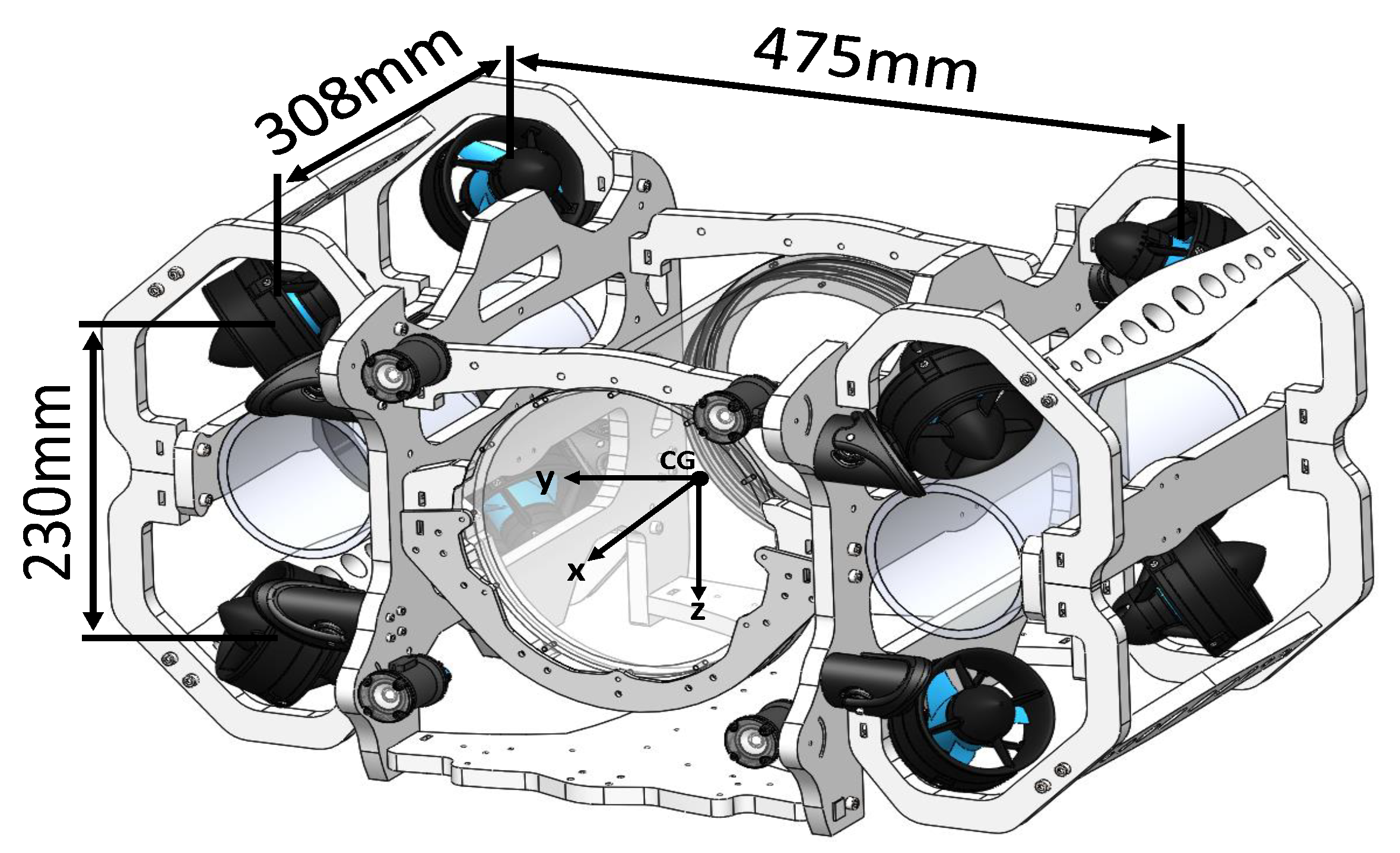
A polyamide Nylon (Nylamid) plate was selected for the construction of the structure due to its properties of resistance to underwater environments, and its lower weight compared to metal materials. The thruster mounts were made by 3D printing using “Onyx”, a filament combined with carbon fiber to provide strength to the mechanical elements. The tubes used in the vehicle are of acrylic. The main tube has an inner diameter of 8.5 in, and supports a maximum immersion of 40 m. This tube contains the electronics, including the autopilot, the Jetson-TX2 card, the ZED camera, the communication modems, to name a few. Two secondary tubes have an inner diameter of 4 in and are used to house the batteries. The connections between the tubes are made through the use of penetrators and connectors, the tubes as well as the thrusters are commercialized by Blue Robotics.

2.1.2. Frame

The structure of the vehicle has a rectangular prismatic shape, allowing the propellers, tubes and lights to be placed in a distributed way. Moreover, the frame takes advantage of the symmetry property, hence the geometric center and the center of gravity are located at the same point, in addition to simplifying values in the inertia matrix. The vehicle has 70 cm by 50 cm of base and 40 cm of height. In Figure 2 we can observe the main structure with the propellers and tubes mounted.

2.1.3. Hydrostatic and Hydrodynamic Considerations with Computational Fluid Dynamics (CFD) Analysis

The designed vehicle, like any other body immersed in a moving fluid, is subject to forces due to the fluid. For the design process, we consider the effects of drag and lift. Drag is defined as the force opposed to movement through the fluid, this drag coefficient was obtained by numerical analysis using the ANSYS Fluid Flow (CFX) software version 20.2. The process was carried out using a control cubic volume Figure 3 (right), the considerations used correspond to a fluid velocity of 1029 ms, at an ambient temperature of 22 °C and a density of 997.86 kg/m³, a simplified vehicle geometry is used which is virtually introduced in the control volume. In the control geometry, the front and rear parallel faces to the analysis plane are considered as input and output respectively. To obtain the values in the translation axis x, y and z, the planes as well as the faces of the control volume are alternated. The approximate drag forces obtained are $F_{dx}=80.36N$, $F_{dy}=85.53N$ and $F_{dz}=102.51N$, and the approximate drag coefficients are $C_{dx}=1.1524$, $C_{dy}=1.23$ and $C_{dz}=1.47$. In Figure 3 the velocity profile of the fluid is observed acting on the surface of the vehicle in the axis of translation y.

The computation of the hydrodynamic parameters (diagonal terms for the added mass parameters as well as linear and non-linear damping parameters) was carried out analytically, following the methodology reported in [48], based on the recommended practice DNV-RP-H103 [49]. The methodology includes the following steps for determining added mass parameters.

• Determine added mass for surge, sway and heave using 3D empirical data.
• Determine added mass for surge, sway and heave using 2D empirical data and strip theory.
• Compute the difference between both methods (obtain a scale factor).
• Determine added mas for roll, pitch and yaw using 2D data and strip theory Scale the results and obtain the added mass parameters.

The added mass parameters computed are listed in

Table 4. Added Mass.

DoF	Added Mass	Value
Surge	$X_{\dot{u}}$	15.4656
Sway	$Y_{\dot{v}}$	14.8887
Heave	$Z_{\dot{w}}$	18.5967
Roll	$K_{\dot{p}}$	0.5527
Pitch	$M_{\dot{q}}$	0.3153
Yaw	$N_{\dot{r}}$	0.6685

. Moreover, the linear and quadratic damping coefficients are presented in

Table 5. Linear & Quadratic Damping.

DoF	Linear Damping	Value	Quadratic Damping	Value
Surge	$X_u$	11.6982	$X_{u|u|}$	73.1138
Sway	$Y_v$	10.7309	$Y_{v|v|}$	67.0684
Heave	$Z_w$	19.4981	$Z_{w|w|}$	121.8630
Roll	$K_p$	0.3151	$K_{p|p|}$	1.1730
Pitch	$M_q$	0.3122	$M_{q|q|}$	0.4357
Yaw	$N_r$	0.6240	$N_{r|r|}$	0.8707

.

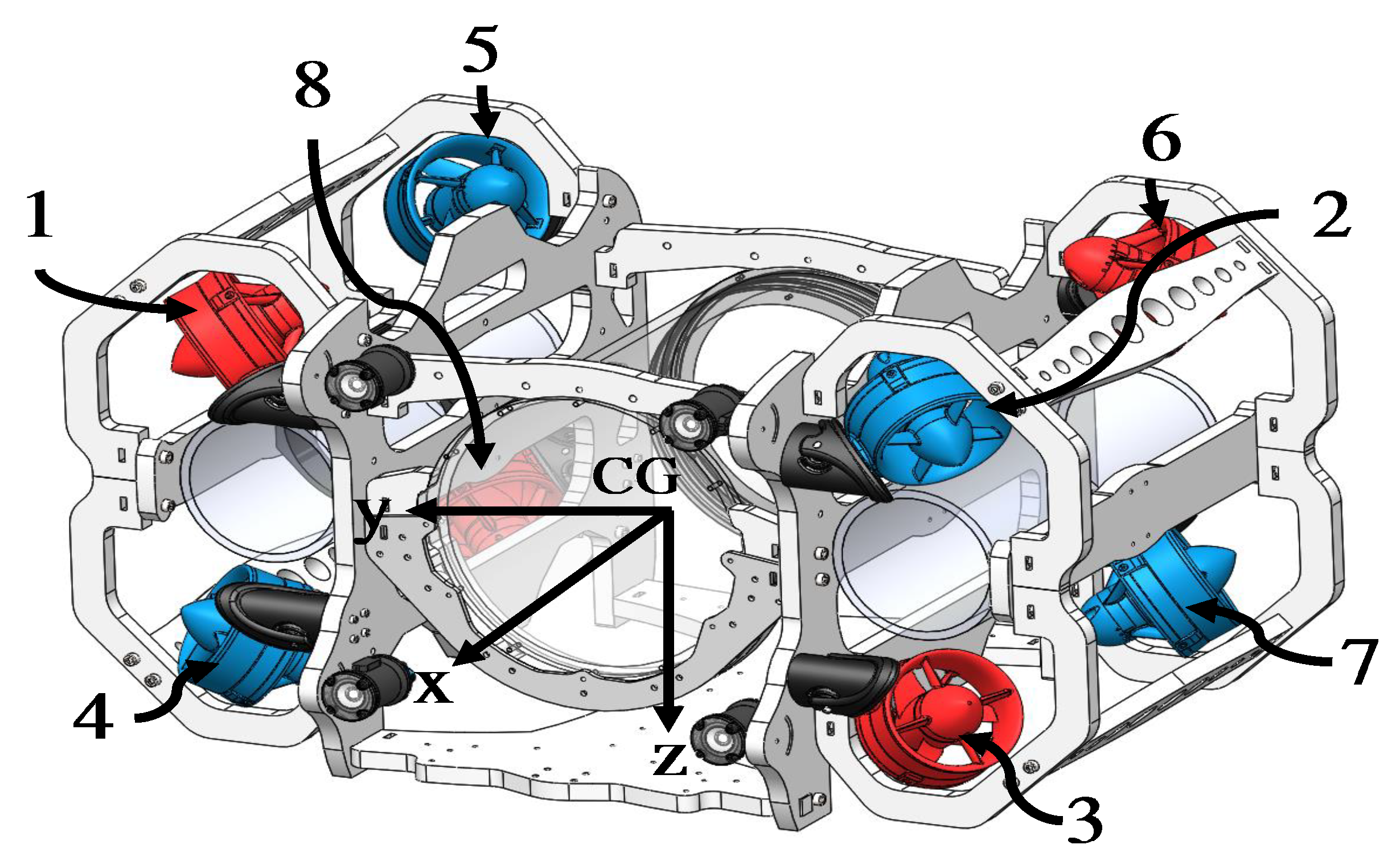
2.1.4. Thrusters Distribution

The eight vehicle’s thrusters are model T200 of BlueRobotics and these are placed at the vertices of the structure (assuming that the vehicle has a rectangular prismatic geometric shape) with an inclination of $\pi /4$ in each of the 3 axes. With this configuration we obtain a greater thrust in each direction, which allows to compensate small disturbances. The distribution of the thrusters is shown in Figure 4, where the propeller of thrusters in red color turn in clockwise direction (CW) and the propeller of thrusters in blue color turn in counter-clockwise direction (CCW). Through the combination of thrusters, the vehicle can generate lateral, vertical, longitudinal displacements, as well as rotational movements in roll, pitch and yaw angles. The vehicle axes are given in the body frame as $X_B$, $Y_B$, $Z_B$.

Figure 5 shows the front view of the vehicle and the location of the front thrusters, labeled as 1, 2, 3 and 4. The movements that the vehicle can perform are:

-

Lateral movement. This is produced by applying a positive signal to thrusters (2, 3, 6, 7) and a negative signal to thrusters (1, 4, 5, 8).

-

Roll movement around the $X_B$ axis. It is achieved through the moments generated by the thrusters. To generate the rotation movement, a positive signal is sent to the thrusters (2, 6, 4, 8) and a negative signal is sent to (3, 7, 1, 5).

Similarly, Figure 6 shows the lateral view of the vehicle, the thrusters distribution and the forces generated on the left side of the vehicle. From this view, the vehicle can perform the following movements:

-

Vertical movement. This happens when a positive signal is sent to the upper thrusters (3, 4, 7, 8) and a negative signal to those located at the bottom (1, 2, 5, 6).

-

Pitch movement around the $Y_B$ axis. This movement is obtained with a positive signal to thrusters (3, 4, 5, 6) and a negative signal to (1, 2, 7, 8).

Finally, Figure 7 shows the distribution of the upper thrusters. The movements observed in this view are

-

Longitudinal movement. This is produced by applying a positive signal to frontal thrusters (1, 2, 3, 4) and a negative signal to rear thrusters (5, 6, 7, 8).

-

Yaw movement around the $Z_B$ axis. This movement is done by applying a positive signal to thrusters (2, 3, 5, 8) and a negative signal to the opposite thrusters (1, 4, 6, 7).

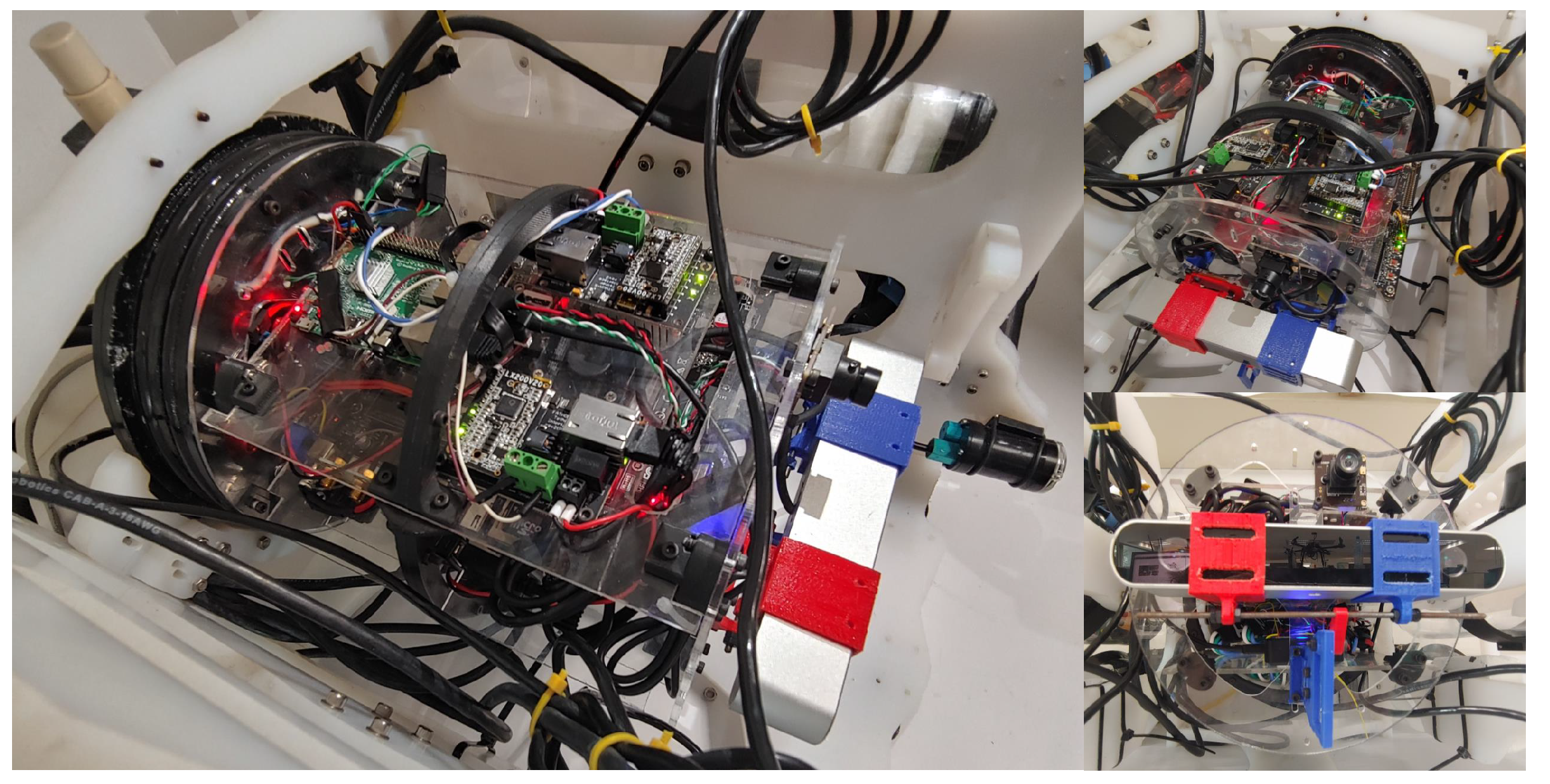
2.2. Electrical and Electronics

The internal electrical system of the underwater vehicle, which is divided into three subsystems. The first one, the position and communication subsystem, which allows the communication of the vehicle’s embedded computers with the control ground station through the MavLink protocol. The second one corresponds to the control subsystem, which is composed by an autopilot, sensors and thrusters. The latter one, the vision subsystem, which is integrated by a low light monocular camera, a stereo vision camera and an image processing system. The vehicle operates with two lipo batteries of 4 cells (4 s) 10 ah connected in parallel. The components of the electrical and electronics system are labeled from C1 to C14 in Figure 8.

2.2.1. Position and Communication

The communication established between the control ground station and the vehicle is carried out through a 100 m ethernet cable (C1) using two Fhatom-X-R1 (C3 and C4), which extend the communication distance between devices connected via the serial protocol. Inside the ethernet cable, one pair of wires is used for the companion computer(Raspberry Pi 3B) (C5), one pair for the Jetson TX2 computer (C13), and another pair for the acoustic locator A1 (C2). The companion computer is connected to a Fathom-X-R1 (C3) module uses the MAVLink protocol, which establishes direct communication between the Pixhawk autopilot (C6) and the control ground station. Another Fathom-X-R1 (C4) module is used to communicate the image processing system (Nvidia’s Jetson TX2 (C13)) with the control ground station via Secure Shell (SSH) protocol. Finally, the acoustic locator A1 (C2), from the WaterLinked company, is part of an underwater positioning system for underwater vehicles.

2.2.2. Control Subsystem

The control subsystem is composed of a Pixhawk autopilot (C6), a temperature sensor (C8), a barometric pressure sensor (C9), speed controllers (ESC (C7)), eight thrusters (C10), in addition to four lights (C11). This subsystem provides measurements from the sensors in the vehicle’s autopilot (inertial measurement unit (IMU), barometer, etc.) and sends pulse-width modulation (PWM) signals to the thrusters, producing translational and rotational displacements. The firmware used in the autopilot is an open source code named ArduSub Version 4.2.0, which is part of the Ardupilot project. The ArduSub firmware has different pre-configured frames, however the configuration for the vehicle developed in this work is not available. Therefore, the file that contains the mixer for the frames is modified (AP_Motors6DOF.cpp), where a new frame corresponding to the motors distribution of the developed vehicle is added.

Table 6. Thrusters Combination.

Thruster	Roll	Pitch	Yaw	Vertical	Forward	Lateral
1	1	$-1$	$-1$	1	1	1
2	$-1$	$-1$	1	1	1	$-1$
3	1	1	1	$-1$	1	$-1$
4	$-1$	1	$-1$	$-1$	1	1
5	1	1	1	1	$-1$	1
6	$-1$	1	$-1$	1	$-1$	$-1$
7	1	$-1$	$-1$	$-1$	$-1$	$-1$
8	$-1$	$-1$	1	$-1$	$-1$	1

shows the necessary thrusters combinations to carry out the translational and rotational movements in the 6 degrees of freedom of the vehicle, this modification was recorded in the (AP_Motors6DOF.cpp) file.

2.2.3. Vision Subsystem

The vision subsystem is composed by 2 cameras. The first one, is a low illumination monocular camera (C12) that allows to observe the environment during the control/manipulation of the vehicle. The second one, a stereo camera model ZEDcam (C14) from StereoLabs is a depth sensor composed of two cameras, which allows to generate a depth image up to 20 m. The SDK provided by Stereolabs allows us to perform different image processing tasks with few lines of code, such as 3D reconstruction, visual odometry, among others. To run the vision algorithms of the SDK it is necessary to have an Nvidia platform, for this reason a Jetson TX2 computer (C13) was incorporated into the vehicle.

2.3. Control Ground Station

The control ground station consists of a computer running the Ubuntu 18.04 LTS operating system, and the Robot Operating System 1 (ROS 1) software with the Melodic Morenia distribution. To interact with the vehicle, the ROS node bluerov_ros_playground from BlueRobotics was used. This node allows us to arm the vehicle, read battery voltage, read IMU values, and send control signals for vehicle movements (vertical, lateral, longitudinal, and roll, pitch, and yaw angle movements). Therefore, the control strategies developed are programmed by creating a new node in ROS and subscribing to the playground node. In addition, the control ground station allows us to run the QGroundControl software to operate the vehicle in manual mode using a joystick. The vehicle is connected to the station through the communication cable and a pair of Fathom-X-R1 modules, one of which is used for the communication with the autopilot and the other for communication with the Jetson TX2 computer.

3. Mathematical Model and Control Strategies

In this section, we present the 6 DOF mathematical model for the underwater vehicle based on the Fossen’s methodology [50]. Also, for control purposes, we present a reduced mathematical model of 3 DOF that includes the roll, pitch and depth dynamics. Finally, the structure of a Robust Proportional Derivative and a Super Twisting controllers are presented.

For the development of the mathematical model as well as the design of control strategies, the following assumptions are stated.

3.1. Assumptions

• In the 3 DOF model, the movement in surge, sway and yaw directions was neglected.
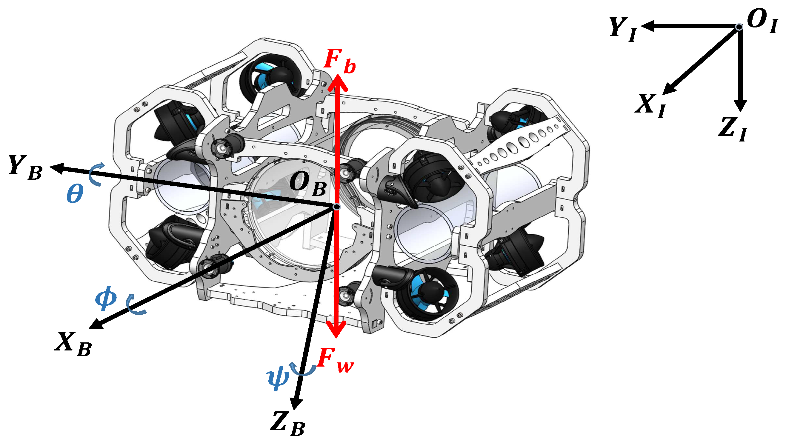
• The vehicle maintains its center of buoyancy above the center of gravity, which provides a positive buoyancy that allows the vehicle to return to the surface in case of power failure.
• The vehicle structure has 3 planes of symmetry.
• In the dynamic model, the disturbances term is added to take into account the effects of tether cable as well as waves.
• The vehicle is considered as a rigid body, without geometric deformations or bending.
• The maximum operation speed of the vehicle is less than 2 m by second.

3.2. 6 DOF Mathematical Model

Consider the underwater vehicle presented in Figure 9. Let us define the inertial and body frame as ${\mathcal{I}}_I=\{O_I,X_I,Y_I,Z_I\}$ and ${\mathcal{I}}_B=\{O_B,X_B,Y_B,Z_B\}$, respectively, $\mathit{\eta }={[x,y,z,\varphi ,\theta ,\psi ]}^{\top }\in {\mathbb{R}}^{6x1}$ describes the vehicle’s position and orientation in the inertial frame, $\mathit{\nu }={[u,v,w,p,q,r]}^{\top }\in {\mathbb{R}}^{6x1}$ denotes the linear and angular velocities in the body frame.

The 6 DOF kinetic and kinematic model expressed in the body frame are given as

$$\begin{array}{cc}\hfill \mathbf{M}\dot{\mathit{\nu }}+\mathbf{C}\left(\mathit{\nu }\right)\mathit{\nu }+\mathbf{D}\left(\mathit{\nu }\right)\mathbf{v}+\mathbf{g}\left(\mathit{\eta }\right)& =\mathit{\tau }\hfill \\ \hfill \dot{\mathit{\eta }}& =\mathbf{J}\left(\mathit{\eta }\right)\mathit{\nu }\hfill \end{array}$$

(1)

where $\mathbf{M}={\mathbf{M}}_{RB}+{\mathbf{M}}_A\in {\mathbb{R}}^{6\times 6}$ represents the inertia matrix with ${\mathbf{M}}_{RB}$ and ${\mathbf{M}}_A$ as rigid-body inertia matrix and added mass matrix respectively, $\mathbf{C}\left(\mathit{\nu }\right)={\mathbf{C}}_{RB}\left(\mathit{\nu }\right)+{\mathbf{C}}_A\left(\mathit{\nu }\right)\in {\mathbb{R}}^{6\times 6}$ define the Coriolis matrix obtained by rigid-body Coriolis matrix ${\mathbf{C}}_{RB}\left(\mathit{\nu }\right)$ and Coriolis matrix for a rigid-body moving through an ideal fluid ${\mathbf{C}}_A\left(\mathit{\nu }\right)$, $\mathbf{D}\left(\mathit{\nu }\right)={\mathbf{D}}_L\left(\mathit{\nu }\right)+{\mathbf{D}}_{NL}\left(\mathit{\nu }\right)\in {\mathbb{R}}^{6\times 6}$ is the damping matrix as the sum of linear damping ${\mathbf{D}}_L\left(\mathit{\nu }\right)$ and nonlinear damping ${\mathbf{D}}_{NL}\left(\mathit{\nu }\right)$, $\mathbf{g}\left(\mathit{\eta }\right)\in {\mathbb{R}}^{6\times 1}$ denotes the vector of gravitational and buoyancy forces, $\mathit{\tau }={[X,Y,Z,K,M,N]}^T\in {\mathbb{R}}^{6\times 1}$ represents the vector of control inputs in the body frame (generalized forces and moments). The kinematic transformation matrix from the vehicle body frame to the inertial frame is given as

$$\mathbf{J}\left(\mathit{\eta }\right)=\left[\begin{array}{cc}\mathbf{R}& 0_{3\times 3}\\ 0_{3\times 3}& \mathbf{T}\end{array}\right]$$

(2)

where

$$\mathbf{R}=\left[\begin{array}{ccc}{C}_{\theta }{C}_{\psi }& S_{\theta }{C}_{\psi }{C}_{\varphi }-C_{\psi }{C}_{\varphi }& S_{\theta }{C}_{\psi }{C}_{\varphi }+S_{\psi }{S}_{\varphi }\\ C_{\theta }{S}_{\psi }& S_{\theta }{S}_{\psi }{S}_{\varphi }+C_{\psi }{C}_{\varphi }& S_{\theta }{S}_{\psi }{C}_{\varphi }-C_{\psi }{S}_{\varphi }\\ -S_{\theta }& C_{\theta }{S}_{\varphi }& C_{\theta }{C}_{\varphi }\end{array}\right]$$

(3)

$$\mathbf{T}=\left[\begin{array}{ccc}1& T_{\theta }{S}_{\varphi }& T_{\theta }{C}_{\varphi }\\ 0& C_{\varphi }& -S_{\varphi }\\ 0& \frac{S_{\varphi }}{C_{\theta }}& \frac{C_{\varphi }}{C_{\theta }}\end{array}\right]$$

(4)

with $C_{\left(·\right)}=cos\left(·\right)$, $S_{\left(·\right)}=sin\left(·\right)$ and $T_{\left(·\right)}=tan\left(·\right)$.

3.3. 3 DOF Mathematical Model

For control purposes, we develop a more detailed 3 DOF mathematical model, where the roll, pitch and depth dynamics are considered. With this in mind, the position, velocities and input vectors are defined as $\mathit{\eta }={\left[z,\varphi ,\theta \right]}^{\top }$, $\mathit{\nu }={\left[w,p,q\right]}^{\top }$, $\mathit{\tau }={\left[Z,K,M\right]}^{\top }$, respectively. The inertia, Coriolis and damping matrix, as well as the vector of gravitational and buoyancy forces, are defined as

$$\mathbf{M}=\left[\begin{array}{ccc}m-Z_{\dot{w}}& m{y}_g-Z_{\dot{p}}& -m{x}_g-Z_{\dot{q}}\\ m{y}_g-K_{\dot{w}}& I_x-K_{\dot{p}}& -I_{xy}-K_{\dot{q}}\\ -m{x}_g-M_{\dot{w}}& -I_{yx}-M_{\dot{p}}& I_y-M_{\dot{q}}\end{array}\right]$$

(5)

where $r_g={[x_g,y_g,z_g]}^{\top }$ is the position vector of the center of gravity CG with respect to the center of the vehicle $O_B$, the $O_B$ is coincident with the CG, this implies that $x_g=y_g=z_g=0$

$$\mathbf{C}\left(\mathit{\nu }\right)=\left[\begin{array}{ccc}{c}_{11}& c_{12}& c_{13}\\ c_{21}& c_{22}& c_{23}\\ c_{31}& c_{32}& c_{33}\end{array}\right]$$

(6)

where

$$\begin{array}{cc}\hfill c_{12}=& -m(p{z}_g-v)-p{Y}_{\dot{p}}-q{Y}_{\dot{q}}-r{Y}_{\dot{r}}-u{Y}_{\dot{u}}-v{Y}_{\dot{v}}-w{Y}_{\dot{w}},\hfill \\ \hfill c_{13}=& -m(q{z}_g+u)+p{X}_{\dot{p}}+q{X}_{\dot{q}}+r{X}_{\dot{r}}+u{X}_{\dot{u}}+v{X}_{\dot{v}}+w{X}_{\dot{w}},\hfill \\ \hfill c_{21}=& m(p{z}_g-v)+p{Y}_{\dot{p}}+q{Y}_{\dot{q}}+r{Y}_{\dot{r}}+u{Y}_{\dot{u}}+v{Y}_{\dot{v}}+w{Y}_{\dot{w}},\hfill \\ \hfill c_{23}=& -p{I}_{xz}-q{I}_{yz}+r{I}_z-p{N}_{\dot{p}}-q{N}_{\dot{q}}-r{N}_{\dot{r}}-u{N}_{\dot{u}}-v{N}_{\dot{v}}-w{N}_{\dot{w}},\hfill \\ \hfill c_{31}=& m(q{z}_g+u)-p{X}_{\dot{p}}-q{X}_{\dot{q}}-r{X}_{\dot{r}}-u{X}_{\dot{u}}-v{X}_{\dot{v}}-w{X}_{\dot{w}},\hfill \\ \hfill c_{32}=& p{I}_{xz}+q{I}_{yz}-r{I}_z+p{N}_{\dot{p}}+q{N}_{\dot{q}}+r{N}_{\dot{r}}+u{N}_{\dot{u}}+v{N}_{\dot{v}}+w{N}_{\dot{w}},\hfill \\ \hfill c_{11}=& c_{22}=c_{33}=0\hfill \end{array}$$

(7)

$$\mathbf{D}\left(\mathit{\nu }\right)=\left[\begin{array}{ccc}-|w|Z_{|w|w}-Z_w& 0& -Z_q\\ 0& -|p|K_{|p|p}-K_p& 0\\ -M_w& 0& -|q|X_{|q|q}-M_q\end{array}\right]$$

(8)

$$\mathbf{g}\left(\mathit{\eta }\right)=\left[\begin{array}{c}(B-W)C_{\theta }{C}_{\varphi }\\ -B{z}_b{C}_{\theta }{S}_{\varphi }\\ -B{z}_b{S}_{\theta }\end{array}\right]$$

(9)

where $r_b={[x_b,y_b,z_b]}^{\top }$ is the position vector of the buoyancy force CB with respect to the center of the vehicle $O_B$, the CB is coincident in the $xy-plane$ with the $O_B$, this implies that $x_g=y_g=0,z_g=-0.1$ since the vehicle is designed with small positive buoyancy. $B=\rho g\nabla$ is the buoyancy force and $W=mg$ the weight of the body, with m the mass of the vehicle, g the acceleration of gravity, $\rho$ the water density and ∇ the volume of fluid displaced by the vehicle. For the 3 DOF dynamic model, the transformation matrix $\mathbf{J}\left(\mathit{\eta }\right)$ is given by

$$\mathbf{J}\left(\mathit{\eta }\right)=\left[\begin{array}{ccc}{C}_{\theta }{C}_{\varphi }& 0& 0\\ 0& 1& T_{\theta }{S}_{\varphi }\\ 0& 0& C_{\varphi }\end{array}\right]$$

(10)

which is nonsingular for $-\pi /2<\theta ,\varphi <\pi /2$. From the kinematic model given in (1), we obtain $\ddot{\mathit{\eta }}=\mathbf{J}\left(\mathit{\eta }\right)\dot{\mathit{\nu }}+\dot{\mathbf{J}}\left(\mathit{\eta }\right)\mathit{\nu }$. Then, the kinetic model denoted in the inertial frame is given as

$${\mathbf{M}}_{\eta }\left(\eta \right)\ddot{\eta }+{\mathbf{C}}_{\eta }\left(\mathit{\nu },\mathit{\eta }\right)\dot{\eta }+{\mathbf{D}}_{\eta }\left(\mathit{\nu },\mathit{\eta }\right)\dot{\eta }+{\mathbf{g}}_{\eta }\left(\mathit{\eta }\right)={\mathit{\tau }}_{\eta }$$

(11)

where

$$\begin{array}{cc}\hfill {\mathbf{M}}_{\eta }\left(\eta \right)& ={\mathbf{J}}^{-T}\left(\mathit{\eta }\right){\mathbf{MJ}}^{-1}\left(\mathit{\eta }\right)\hfill \\ \hfill {\mathbf{C}}_{\eta }\left(\mathit{\nu },\mathit{\eta }\right)& ={\mathbf{J}}^{-T}\left(\mathit{\eta }\right)\left[\mathbf{C}\left(\mathit{\nu }\right)-{\mathbf{MJ}}^{-1}\left(\mathit{\eta }\right)\dot{\mathbf{J}}\left(\mathit{\eta }\right)\right]{\mathbf{J}}^{-1}\left(\mathit{\eta }\right)\hfill \\ \hfill {\mathbf{D}}_{\eta }\left(\mathit{\nu },\mathit{\eta }\right)& ={\mathbf{J}}^{-T}\left(\mathit{\eta }\right)\mathbf{D}\left(\mathit{\nu }\right){\mathbf{J}}^{-1}\left(\mathit{\eta }\right)\hfill \\ \hfill {\mathbf{g}}_{\eta }\left(\mathit{\eta }\right)& ={\mathbf{J}}^{-T}\left(\mathit{\eta }\right)\mathbf{g}\left(\mathit{\eta }\right)\hfill \\ \hfill {\mathit{\tau }}_{\eta }\left(\mathit{\eta }\right)& ={\mathbf{J}}^{-T}\left(\mathit{\eta }\right)\mathit{\tau }={\left[Z_{\eta },K_{\eta },M_{\eta }\right]}^{\top }\hfill \end{array}$$

The dynamic model given in Equation (11) can be rewritten as

$$\ddot{\mathit{\eta }}={\mathbf{M}}_{\eta }{\left(\mathit{\eta }\right)}^{-1}\left[-{\mathbf{C}}_{\eta }\left(\mathit{\nu },\mathit{\eta }\right)\dot{\mathit{\eta }}-{\mathbf{D}}_{\eta }\left(\mathit{\nu },\mathit{\eta }\right)\dot{\mathit{\eta }}-{\mathbf{g}}_{\eta }\left(\mathit{\eta }\right)+{\mathit{\tau }}_{\eta }\right]$$

(12)

Defining $\mathbf{\Gamma }={\left[{\Gamma }_z,{\Gamma }_{\varphi },{\Gamma }_{\theta }\right]}^{\top }$ as an equivalent disturbance with the following structure

$$\begin{array}{cc}\hfill \mathbf{\Gamma }=& {\mathbf{M}}_{\eta }{\left(\mathit{\eta }\right)}^{-1}\left[-{\mathbf{C}}_{\eta }\left(\mathit{\nu },\mathit{\eta }\right)\dot{\mathit{\eta }}-{\mathbf{D}}_{\eta }\left(\mathit{\nu },\mathit{\eta }\right)\dot{\mathit{\eta }}-{\mathbf{g}}_{\eta }\left(\mathit{\eta }\right)\right]\hfill \\ \hfill & +{\mathbf{M}}_{\eta }{\left(\mathit{\eta }\right)}^{-1}{\mathit{\tau }}_{\eta }-{\mathbf{M}}_{\alpha }{\mathit{\tau }}_{\eta }\hfill \end{array}$$

(13)

with ${\mathit{M}}_{\alpha }=\mathrm{diag}\left(m-Z_{\dot{w}},I_x-K_{\dot{p}},I_y-M_{\dot{q}}\right)=\mathrm{diag}\left(M_z,M_{\varphi },M_{\theta }\right)$. Then, the underwater vehicle dynamical model given in Equation (12) can be rewritten as

$$\ddot{\mathit{\eta }}={\mathbf{M}}_{\alpha }{\mathit{\tau }}_{\eta }+\mathbf{\Gamma }$$

(14)

which is equivalent to

$$\begin{array}{c}\ddot{z}=M_z{Z}_{\eta }+{\Gamma }_z\\ \ddot{\varphi }=M_{\varphi }{K}_{\eta }+{\Gamma }_{\varphi }\\ \ddot{\theta }=M_{\theta }{M}_{\eta }+{\Gamma }_{\theta }\end{array}$$

(15)

Finally, for control strategies design purpose, dynamics given by Equation (15) are rewritten in a general form as

$${\ddot{\chi }}_i=M_i{u}_i+{\Gamma }_i,i=z,\varphi ,\theta$$

(16)

and $u_1=Z_{\eta },u_2=K_{\eta },u_3=M_{\eta }$. Below, we present two classical control strategies, Super Twisting and Robust PD, that were applied to the underwater vehicle. It is worth mentioning that the main focus of the manuscript is not the development of control strategies. Conversely, to show that the vehicle is able to realize stabilization and trajectory tracking tasks even when classical control strategies are applied.

3.4. Thruster Configuration and Control Allocation

Consider the vector of forces $\mathbf{F}={\left[F_1,F_2,\dots ,F_8\right]}^{\top }$, where $F_i,i=1,\dots ,8$ is the force applied to each thruster. The vector of generalized forces and moments $\mathit{\tau }={[X,Y,Z,K,M,N]}^{\top }$, previously defined in Section 3.2, can be expressed as

$$\mathit{\tau }=\mathbf{T}\left(\mathbf{a}\right)\mathbf{F}=\mathbf{T}\left(\mathbf{a}\right)\mathbf{K}\mathbf{u}$$

(17)

where $\mathbf{T}\left(\mathbf{a}\right)=[{\mathbf{t}}_{\mathbf{1}},{\mathbf{t}}_{\mathbf{2}},\dots {\mathbf{t}}_{\mathbf{8}}]\in {\mathbb{R}}^{6\times 8}$ is the thrust configuration matrix, $\mathbf{a}\in {\mathbb{R}}^{8\times 1}$ is the thrust rotation angle vector, $\mathbf{K}=diag[K_1,K_2,\dots ,K_8]\in {\mathbb{R}}^{8\times 1}$ is the thrust coefficient matrix and $\mathbf{u}={[u_1,u_2,\dots ,u_8]}^{\top }$ is the vector of inputs to the thrusters. The rotation angles for all thrusters are $\pi /4$ in each of the 3 axis. Besides, each component of the thrust configuration matrix can be obtained as

$${\mathbf{t}}_{\mathbf{i}}=\left[\begin{array}{c}{\mathbf{f}}_{\mathbf{i}}\\ {\mathbf{r}}_{\mathbf{i}}\times {\mathbf{f}}_{\mathbf{i}}\end{array}\right]=\left[\begin{array}{c}{F}_{x_i}\\ F_{y_i}\\ F_{z_i}\\ F_{x_i}{l}_{y_i}-F_{y_i}{l}_{z_i}\\ F_{x_i}{l}_{z_i}-F_{z_i}{l}_{x_i}\\ F_{y_i}{l}_{x_i}-F_{x_i}{l}_{y_i}\end{array}\right],i=1,\dots ,8$$

(18)

where ${\mathbf{f}}_{\mathbf{i}}={[F_{x_i},F_{y_i},F_{z_i}]}^{\top }$ is the force vector and ${\mathbf{r}}_{\mathbf{i}}={[l_{x_i},l_{y_i},l_{z_i}]}^{\top }$ are the moment arms for the i-th thruster. From Figure 1, the moment arms relative to center of gravity are listed in

Table 7. Moment arms for each thruster.

${\mathit{T}}_{\mathit{i}}$	${\mathit{l}}_{{\mathit{x}}_{\mathit{i}}}\left(\mathbf{mm}\right)$	${\mathit{l}}_{{\mathit{y}}_{\mathit{i}}}\left(\mathbf{mm}\right)$	${\mathit{l}}_{{\mathit{z}}_{\mathit{i}}}\left(\mathbf{mm}\right)$
$T_1$	154	237.5	−115
$T_2$	154	−237.5	−115
$T_3$	154	−237.5	115
$T_4$	154	237.5	115
$T_5$	−154	237.5	−115
$T_6$	−154	−237.5	−115
$T_7$	−154	−237.5	115
$T_8$	−154	237.5	115

for each thruster.

Finally, the thrust configuration matrix $\mathbf{T}\left(\mathbf{a}\right)$ for the vehicle developed is given by

$$\mathbf{T}\left(\mathbf{a}\right)=\left[\begin{array}{cccccccc}0.707& 0.707& 0.707& 0.707& -0.707& -0.707& -0.707& -0.707\\ 0.707& -0.707& -0.707& 0.707& 0.707& -0.707& -0.707& 0.707\\ 0.707& 0.707& -0.707& -0.707& 0.707& 0.707& -0.707& -0.707\\ 0.249& -0.249& 0.249& -0.249& 0.249& -0.249& 0.249& -0.249\\ -0.190& -0.190& 0.190& 0.190& 0.190& 0.190& -0.190& -0.190\\ -0.059& 0.059& 0.059& -0.059& 0.059& -0.059& -0.059& 0.059\end{array}\right]$$

(19)

In Equation (19), the columns represent the thrusters 1 to 8, while the rows represent the components in x, y, z and $roll$, $pitch$ and $yaw$ respectively.

The control allocation method computes the input signal $\mathbf{u}$ that needs to be applied to each thruster from the control input vector $\mathit{\tau }$. Then, from Equation (17), the vector of inputs to the thruster can be computed as

$$\mathbf{u}={\mathbf{K}}^{-1}{\mathbf{T}}^{+}\mathit{\tau }$$

(20)

where ${\mathbf{T}}^{+}=\mathbf{T}{(\mathbf{a})}^{\top }{(\mathbf{T}(\mathbf{a})\mathbf{T}{(\mathbf{a})}^{\top })}^{-1}$ is a pseudo-inverse matrix due to the thrust configuration matrix $\mathbf{T}\left(\mathbf{a}\right)$ is non-square.

3.5. Robust PD Control Strategy

In order to deal with the lumped disturbances presents in the underwater vehicle given in Equation (14), a robust compensator based on a robust filter to reduce the effects of external disturbances [51,52] is presented in this section. First, we define the tracking error as $e_{{\chi }_i}={\chi }_i-{\chi }_{i_d}$, ${\dot{e}}_{{\chi }_i}={\dot{\chi }}_i-{\dot{\chi }}_{i_d}$ and ${\ddot{e}}_{{\chi }_i}={\ddot{\chi }}_i-{\ddot{\chi }}_{i_d}$. Then, the subsystem error for dynamics (16) is expressed in compact form as

$${\ddot{e}}_{{\chi }_i}=M_i{u}_i+{\Gamma }_i-{\ddot{\chi }}_{i_d}$$

(21)

The robust control strategy is composed of a nominal controller (a proportional derivative in this case) and a robust term. The PD control strategy has been successfully implemented in underwater vehicles [53,54,55], for this reason is chosen as nominal controller. Therefore, the control signal in time-domain is given as

$$u_i=u_i^N+u_i^{RC}$$

(22)

where the nominal control $u_i^N$ is given as

$$u_i^N=-\frac{K_{i1}{e}_{{\chi }_i}+K_{i2}{\dot{e}}_{{\chi }_i}+{\ddot{\chi }}_{i_d}}{M_i}$$

(23)

with $K_{i1}$ and $K_{i2}$ positive gains to be determined. Substituting the control law $u_i$ in (21) we obtain

$${\dot{\mathbf{e}}}_{\mathbf{i}}={\mathbf{A}}_{\mathbf{i}}{\mathbf{e}}_i+\mathbf{B}\left(u_i^{RC}+{\Gamma }_i\right)$$

(24)

where

$${\mathbf{A}}_{\mathbf{i}}=\left[\begin{array}{cc}0& 1\\ -K_{i1}& -K_{i2}\end{array}\right],\mathbf{B}=\left[\begin{array}{c}0\\ 1\end{array}\right],{\mathbf{e}}_{\mathbf{i}}={\left[e_{{\chi }_i}{\dot{e}}_{{\chi }_i}\right]}^{\top }$$

(25)

and the robust term $u_i^{RC}$ in Laplace-domain is given as

$$u_i^{RC}\left(s\right)=-\frac{F_i^{RC}\left(s\right){\Gamma }_i\left(s\right)}{M_i}$$

(26)

where s is the Laplace operator. The term $F_i^{CR}\left(s\right)$ is based in the following second-order filter [56],

$$F_i^{RC}\left(s\right)=\frac{p_i^2}{{(s+p_i)}^2}$$

(27)

where the term $p_i$ is a parameter of the filter. It is assumed that the robust filters possess the following property [57,58]: a larger $p_i$ would have sufficiently wide frequency bandwidth and satisfy that $|F_i^{RC}\left(s\right)|\approx 1$. In order to ensure that the tracking error vector ${\mathbf{e}}_{\mathbf{i}}$ is bounded, the following theorem is stated.

Theorem 1.

Assume that the initial tracking error ${\mathbf{e}}_{\mathbf{i}}\left(0\right)$ is bounded. For positive constants $T^{\times }$, ϵ, and for positive filter parameters $p_i$, if the robust compensator is chosen as in Equation (26), then the tracking error is bounded as ${\Vert {\mathbf{e}}_{\mathbf{i}}\Vert }_{\infty }\le ϵ\forall t\ge T^{\times }$ [56].

Proof. 

From solution of Equation (24), the following solution is obtained

$${\Vert {\mathbf{e}}_{\mathbf{i}}\Vert }_{\infty }\le {\gamma }_{\left(0\right)}+{\delta }_F{\Vert {\Gamma }_i\Vert }_{\infty }$$

(28)

where ${\gamma }_{\left(0\right)}={max}_j{sup}_{t\ge 0}|c_{j}exp\left({\mathbf{A}}_{\mathbf{i}}t\right){\mathbf{e}}_{\mathbf{i}}\left(0\right)|$ and ${\delta }_F={\Vert {\left(s{\mathbf{I}}_{\mathbf{2}\times \mathbf{2}}-{\mathbf{A}}_{\mathbf{i}}\right)}^{-1}{\mathbf{B}}_{\mathbf{i}}\left(1-F_i^{RC}\left(s\right)\right)\Vert }_1$. Assuming that the lumped disturbance term ${\Gamma }_i$ is bounded, then there exists positive constants ${\xi }_0$, ${\xi }_1$ and ${\xi }_2$ that fulfill

$$|{\Gamma }_i|\le {\xi }_0+{\xi }_1{\Vert {\mathbf{e}}_{\mathbf{i}}\Vert }_{\infty }+{\xi }_2{\Vert {\mathbf{e}}_{\mathbf{i}}\Vert }_{\infty }^2$$

(29)

If ${\delta }_F$ is small enough ($|F_i^{RC}\left(s\right)|\approx 1$) such that the following inequality is satisfied

$$\left({\xi }_1+{\xi }_2{\Vert {\mathbf{e}}_{\mathbf{i}}\Vert }_{\infty }\right)\left(\sqrt{{\delta }_F}+{\delta }_F\right)\le 1$$

(30)

then the lumped disturbances is bounded as $|{\Gamma }_i|\le {\xi }_4/\sqrt{{\delta }_F}$ for a positive ${\delta }_4$. Notice that Equation (28) can be rewritten as

$${\Vert {\mathbf{e}}_{\mathbf{i}}\Vert }_{\infty }\le {\gamma }_{\left(0\right)}+\sqrt{{\delta }_F}{\xi }_4$$

(31)

Then, we conclude that the tracking error is bounded, i.e., ${\Vert {\mathbf{e}}_{\mathbf{i}}\Vert }_{\infty }\le ϵ\forall t\le T^{\times }$. The attraction region is given by

$$\left\{{\mathbf{e}}_{\mathbf{i}}:{\Vert {\mathbf{e}}_{\mathbf{i}}\Vert }_{\infty }\le {\xi }_5/\sqrt{{\delta }_F}\right\}$$

(32)

where ${\xi }_5$ is defined as

$${\xi }_5=\frac{1}{{\xi }_2+{\xi }_2\sqrt{{\delta }_F}}-\frac{{\xi }_1\sqrt{{\delta }_F}}{{\xi }_2}$$

(33)

Finally, from Equations (28) and (32) it is concluded that the tracking error ${\mathbf{e}}_{\mathbf{i}}$ remains in the attractive region if the initial conditions fulfill

$${\Vert \mathbf{e}\left(0\right)\Vert }_{\infty }\le {\xi }_5/\sqrt{{\delta }_F}$$

(34)

 □

Remark 1.

For the implementation of control signal $u_i$, the equivalent disturbance ${\Gamma }_i$ cannot be measured directly, then it can be derived from (21) as

$${\Gamma }_i={\ddot{e}}_{{\chi }_i}-M_i{u}_i+{\ddot{\chi }}_{i_d}$$

(35)

Then, from Equations (35) and (26), the following realization is obtained in time-domain for $u_i^{RC}$ with auxiliary state variables ${\xi }_{i_1}$ and ${\xi }_{i_2}$

$$\begin{array}{c}\hfill \begin{array}{cc}\hfill {\dot{\xi }}_{i_1}& =-p_i{\xi }_{i_1}-p_i^2{e}_{i1}+M_i{u}_i\hfill \\ \hfill {\dot{\xi }}_{i2}& =-p_i{\xi }_{i2}+{\xi }_{i1}+2p_i{e}_{i1}\hfill \\ \hfill u_i^{RC}& =\frac{p_i^2({\xi }_{i2}-e_{i1})}{M_i}\hfill \end{array}\end{array}$$

(36)

3.6. Super Twisting Control Strategy

The super twisting controller is a second order sliding mode that reduce the chaterring effect in the control signal and enable us to reject lumped disturbances. Consider the following sliding mode surface

$$s_i={\dot{e}}_{{\chi }_i}+{\beta }_i{e}_{{\chi }_i},{\beta }_{i1}>0$$

(37)

where the tracking error $e_{{\chi }_i}$ and its temporal derivative were previously defined. Notice that if the sliding surface $s_i=0$, then the tracking error converges asymptotically to zero. With the dynamics given in Equation (16), the temporal derivative of the sliding surface is given by

$${\dot{s}}_i=M_i{u}_i+{\Gamma }_i-{\ddot{\chi }}_{i_d}$$

(38)

Then, the following control law based in the super twisting algorithm is proposed

$$u_i=\frac{1}{M_i}\left({\ddot{\chi }}_{i_d}-{\beta }_i{\dot{e}}_{{\chi }_i}-k_{s_{i1}}{|s_i|}^{\frac{1}{2}}sign\left(s_i\right)-k_{s_{i2}}{\int }_0^{t}sign\left(s_i\right)d\tau \right)$$

(39)

with gains $k_{s_{i1}}$ and $k_{s_{i2}}$ to be defined latter. Substituting the control law (39) in the temporal derivative of the sliding surface, we obtain

$${\dot{s}}_i=-k_{s_{i1}}{|s_i|}^{\frac{1}{2}}sign\left(s_i\right)-k_{s_{i2}}{\int }_0^{t}sign\left(s_i\right)d\tau +{\Gamma }_i$$

(40)

To guarantee the stability of the tracking error, it is necessary to guarantee the convergence of the sliding surface to zero.

Theorem 2.

Consider the second order system given in Equation (16) and the sliding surface defined in (37). Assume that the derivative with respect to time of the disturbance ${\Gamma }_i$ is globally bounded as $|{\dot{\Gamma }}_i|<{\Gamma }_i^{+}$ with ${\Gamma }_i^{+}>0$. If the control signal is proposed as in Equation (39), and the gains $k_{s_{i1}}$ and $k_{s_{i2}}$ are selected according to

$$k_{s_{i1}}>0,k_{s_{i2}}>k_{s_{i1}}\frac{6{\Gamma }_i^{+}+4{\left(\frac{{\Gamma }_i^{+}}{k_{s_{i1}}}\right)}^2}{2k_{s_{i1}}}$$

(41)

then, the sliding surface defined (37) converges to zero ($s_i=0$) in a finite-time T and the tracking error $e_{{\chi }_i}$ is asymptotically stable [29,30].

Proof. 

A sketch of the stability analysis based in Lyapunov theory is presented below. Consider the following change of variable

$$\mathit{\sigma }=\left[{\sigma }_1{\sigma }_2\right]={\left[{|s_i|}^{\frac{1}{2}}sign\left(s_i\right)-k_{s_{i2}}{\int }_0^{t}sign\left(s_i\right)d\tau +{\Gamma }_i\right]}^{\top }$$

(42)

Let us define the following Lyapunov candidate function

$$V={\mathit{\sigma }}^{\top }\mathbf{P}\mathit{\sigma }$$

(43)

where

$$\mathbf{P}={\mathbf{P}}^T=\left[\begin{array}{cc}2k_{s_{i2}}+\frac{1}{2}{k}_{s_{i1}}^2& -\frac{1}{2}{k}_{s_{i1}}\\ -\frac{1}{2}{k}_{s_{i1}}& 1\end{array}\right]$$

(44)

Notice that P matrix is positive definite if $k_{s_{2i}}>0$. The time derivative of (43) is given as

$$\dot{V}=-\frac{1}{|{\sigma }_1|}{\mathit{\sigma }}^{\top }\mathbf{Q}\mathit{\sigma }+{\dot{\Gamma }}_i\mathit{\varrho }\mathit{\sigma }$$

(45)

where

$$\mathbf{Q}={\mathbf{Q}}^{\top }=\left[\begin{array}{cc}\frac{k_{s_{i1}}}{2}\left(k_{s_{i1}}^2+2k_{s_{i2}}\right)& -\frac{k_{s_{i1}}^2}{2}\\ -\frac{k_{s_{i1}}^2}{2}& \frac{k_{s_{i1}}}{2}\end{array}\right],\mathit{\varrho }=\left[-k_{s_{i1}}2\right]$$

(46)

For Equation (45), we can obtain

$$\begin{array}{cc}\hfill \dot{V}\le & -\frac{1}{|{\sigma }_1|}{\mathit{\sigma }}^{\top }\mathbf{Q}\mathit{\sigma }+|{\dot{\Gamma }}_i\mathit{\varrho }\mathit{\sigma }|\hfill \\ \hfill \le & -\frac{1}{|{\sigma }_1|}{\mathit{\sigma }}^{\top }\overline{\mathbf{Q}}\mathit{\sigma }\hfill \end{array}$$

(47)

where

$$\overline{\mathbf{Q}}=\left[\begin{array}{cc}\frac{k_{s_{i1}}}{2}\left(k_{s_{i1}}^2+2k_{s_{i2}}\right)-k_{s_{i1}}{\Gamma }_i^{+}& -\frac{k_{s_{i1}}^2}{2}-{\Gamma }_i^{+}\\ -\frac{k_{s_{i1}}^2}{2}-{\Gamma }_i^{+}& \frac{k_{s_{i1}}}{2}\end{array}\right]$$

(48)

The matrix $\overline{\mathbf{Q}}$ is positive definite if the gains are chosen as in Equation (41). Therefore, the derivative of the Lyapunov function is negative definite. Moreover, from the fact that

$${\lambda }_{min}\left(\mathbf{P}\right){\Vert \mathit{\sigma }\Vert }^2\le V\le {\lambda }_{max}\left(\mathbf{P}\right){\Vert \mathit{\sigma }\Vert }^2$$

(49)

where ${\lambda }_{min}\left(\mathbf{P}\right)$ and ${\lambda }_{max}\left(\mathbf{P}\right)$ denote the minimum and maximum eigenvalues of P matrix, we can obtain

$$|{\sigma }_1|\le \Vert \mathit{\sigma }\Vert \le \frac{V^{1/2}}{{\lambda }_{min}{\left(\mathbf{P}\right)}^{1/2}}$$

(50)

Then, Equation (47) can be rewritten as

$$\dot{V}\le -\zeta V^{1/2}$$

(51)

where $\zeta =\frac{{\lambda }_{min}{\left(\mathbf{P}\right)}^{1/2}{\lambda }_{min}\left(\overline{\mathbf{Q}}\right)}{2{\lambda }_{max}\left(\mathbf{P}\right)}$. From Equation (51), it follows that V and $\mathit{\sigma }$ converge to zero in a finite time T bounded by $T\le \frac{2V{\left(0\right)}^{1/2}}{\zeta }$. It is worth mentioning that if $\mathit{\sigma }\to \mathbf{0}$, then the sliding surface $s_i$ converges to zero in finite time. □

4. Results

This section introduces the final results for the design and construction of the underwater vehicle. Moreover, simulation and the experimental results for a Super Twisting and Robust PD control strategies are implemented for the roll, pitch and depth dynamics of the vehicle. Furthermore, to probe the vision characteristics, a 3D reconstruction was conducted in real time.

4.1. Underwater Vehicle Platform

Once the frame of the underwater vehicle was assembled, as shown in Figure 2, the vehicle’s electrical connections were carried out. Figure 10 shows the main tube with the electronic components of the position and communication, control and vision subsystems. The connections of each subsystem were tested individually and together before closing the main tube.

Once the electronic connections of the underwater vehicle were completed, it was fully assembled as shown in Figure 11. After that, a vacuum test was performed successfully.

As a safety factor, a common practice is to design an AUV with positive buoyancy, guaranteeing that if they have any failure, it will tend to rise to the surface of the water and thus be able to recover it. Also, buoyancy should not be excessive because the vehicle will consume more energy to achieve immersion, reducing autonomy time. The bouyancy tests were conducted in a circular swimming pool, where the prototype was placed on the surface and it was verified that it has positive buoyancy. The vehicle keeps approximately $8\%$ of its body out of the water when it is at rest, as is observed in Figure 12.

The first displacement test was carried out in manual mode, where it was possible to observe the correct movement of the vehicle in its 6 DOF. In Figure 13 we can observe the vehicle inside a swimming pool when it is operated manually. The behavior of the vehicle in manual operation can be appreciated in the following video: https://youtu.be/C_jpOa8Ytys (accessed on 25 August 2023).

4.2. Trajectory Tracking Results

In order to observe the vehicle’s performance in closed-loop, three sets of experiments were proposed for the roll and pitch angles, as well as the for the depth dynamics, where two control strategies were applied: a super twisting and a robust PD controller. The experiments sets are described below.

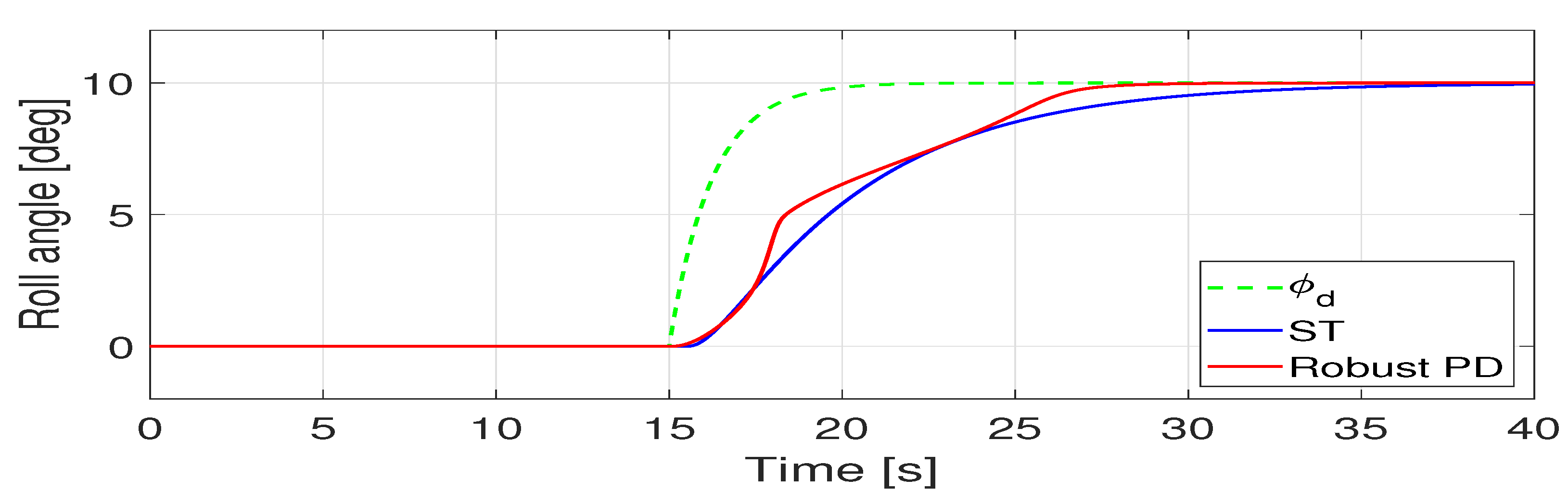
• Experiments A. In these experiments, the vehicle starts in zero as initial condition for the three dynamics (roll, pitch and depth) and the vehicle tracks a desired reference. For the roll and pitch angles, a reference signal of 10 degrees was requested at time 15 s. For the depth dynamics, a reference signal of 20 cm is requested from time instant zero. The objective in these experiments is to show the vehicle’s performance from rest.
• Experiments B. This set of experiments was conducted for roll and pitch angles only. For both dynamics, the signal reference is a square trajectory with a first order low-pass filter. In these experiments the vehicle moves from rest to a reference of −5 degrees and after that it returns back to rest. The objective is to observe the vehicle’s performance when it is stabilized at zero, starting from a non-zero initial condition.
• Experiments C. In this test the vehicle was stabilized at a reference of 10 degrees in roll angle, during the test in two time instants a extra load of 200 g is placed in the vehicle (at one edge of the vehicle) and removed in approximately fifty seconds. This virtual change in system parameters generates a moment of $0.51N$ in the center of gravity, opposite to the $roll$ angle. The objective of this experiment is to show the robustness of the control strategy when an extra load is added to the vehicle. In this experiment the robust PD controller was tested only.

It is worth mentioning that only the conditions of Experiments A were simulated. This simulation enables us to conduct a comparison between the mathematical model and the real-time platform. Experiments A, B and C were conducted in real-time to observe the underwater vehicle’s performance under different operating environments.

The control parameters for simulation and experimentation of the ST controller are shown in

Table 8. Parameters ST Controller.

Simulation Gains				Experimental Gains
Dynamic	${\beta }_i$	$k_{s_{i1}}$	$k_{s_{i2}}$	${\beta }_i$	$k_{s_{i1}}$	$k_{s_{i2}}$
z	0.8	1.8	0.1	0.4	4	0.6
$roll$	0.4	0.1	0.01	0.6	1.5	0.4
$pitch$	0.4	0.15	0.02	0.5	3.5	0.8

. In addition,

Table 9. Parameters Robust PD Controller.

Simulation Gains				Experimental Gains
Dynamic	$K_{i1}$	$K_{i2}$	$p_i$	$K_{i1}$	$K_{i2}$	$p_i$
z	3	1.5	0.7	1.5	0.5	0.3
$roll$	0.9	0.35	0.5	8	1.4	1
$pitch$	0.5	0.25	0.5	2.5	0.5	1

shows the parameters of the Robust PD controller for the simulation and experimentation cases.

4.2.1. Simulation Results

Below, the description of the first set of experiments is described for roll, pitch angle as well as depth dynamic.

Experiments A

In this first set of experiments, a reference signal of 10 degrees was requested at a time of 15 s for $roll$ and $pitch$ dynamics. A similar behavior is observed in the response of both controllers for $roll$ in Figure 14, but the Robust PD control reaches the reference in less time.

Now in Figure 15 we can observe the behavior of the ST and Robust PD controllers for a $pitch$ reference, we can see that the ST controller response is faster than the Robust PD controller, however, the Robust PD controller converges more quickly to the requested reference.

The last simulation test is shown in Figure 16, it is observed an overshoot for the ST controller in the z dynamic, if this overshoot is reduced, the time to reach the reference becomes too large compared to the Robust PD controller.

4.2.2. Experimental Results

In order to observe the vehicle’s performance in closed-loop, three sets of experiments were conducted for the $roll$ and $pitch$ angles, as well as the for the depth dynamic, where two control strategies were applied; a super twisting and a robust PD controllers.

Experiments A

The experimental results for the first set of experiments are presented in Figure 17 and Figure 18. We can observe that when the super twisting controller is applied, the convergence time is slow. When the experiment is conducted with the robust PD controller, we can note that the controller exhibits a better performance and the angles are close to the reference signal.

The control input signal for both previous experiments are presented, in Figure 19 and Figure 20 we can appreciate the thrust force signal for $roll$ and $pitch$ respectively, the range of signal values are expressed in $Nm$ and is calculated using a relationship in the performance charts for T200 thrusters provided by Bluerobotics and the distance from the centre of gravity and the location of the thrusters.

In Figure 21 an overshot can be observed when the super twisting controller is applied to the depth dynamics for an immersion task. In this case, the reference signal was 20 cm. In contrast, when the robust PD is applied, the vehicle tracks the desired reference successfully.

Finally, in Figure 22 we can observe the forces produced by input signals for the z dynamics, both controllers maintain a similar control signal, however, the $ST$ controller shows an overshoot during its reaching time.

Experiments B

A second set of experiments were conducted only for roll and pitch angles, as is shown in Figure 23 and Figure 24. In these experiments, the robust PD and ST controllers were used. The reference signal was a square trajectory with a first order low pass filter. It can be observed that the references includes negative angles in contrast to previous experiments. A satisfactory response for Robust PD was obtained, and a slightly more oscillating response. However, the amplitude of the oscillations is about 1 degree.

In this case, conventional strategies were chosen to be applied.

Experiments C

In Figure 25 we can see the robustness behavior of the Robust PD controller. In this test, the vehicle was stabilized at a reference of 10 degrees on $roll$, during the test time, a load of 200 g was applied and removed at the edge of the vehicle, generating a disturbance of approximately 1.5 degrees in roll angle. The moment opposing to the control signal is $0.51N$, the negative peaks indicate when the load was placed while positive peaks indicate when the load was removed.

4.2.3. Guidelines for Control Parameters Tuning

The following items show how the parameters of both controllers are determined.

Super Twisting Controller

• First, a not so large ${\beta }_i$ is chosen keeping $k_{s_{i1}}=1$ and $k_{s_{i2}}=0$, since it was observed that a too large ${\beta }_i$ generates oscillations in the vehicle’s dynamics. The parameter ${\beta }_i$ affects the convergence velocity of the system.
• The next step is to select a $k_{s_{i1}}$ with $k_{s_{i2}}=0$, since the behavior is similar to the proportional gain of a classical Proportional Integral Derivative (PID) controller, this was chosen to ensure that the convergence to the reference should be in a time no longer than 20 s.
• Finally, the gain $k_{s_{i2}}$ is chosen, helping us to reduce the error in steady state.

Robust PD Controller

• First, a gain adjustment was made for the classic PD controller, the proportional gain $K_{i1}$ is selected, large enough to make the system respond with $K_{i2}=0$.
• With proportional gain $K_{i1}$ selected, a proportional gain $K_{i2}$ was chosen to reduce overshoot in the dynamics response.
• Finally, a gain $p_i$ was selected for the robust term, which helps to compensate the equivalent disturbances ${\Gamma }_i$. The parameter $p_i$ can be increased monotonically until a successfully performance is observed [51].

4.3. 3D Reconstruction

The final 3D reconstruction result is presented in Figure 26. In this experiment, we obtain a 3D model of a plastic cover located on the edge of a circular swimming pool. The result was obtained using the ZEDfu which is a 3D scanning application of StereoLabs that captures 3D models of a scene in real-time. This result enables us to conduct quick analysis of the environment.

A zoom in the 3D model is presented in Figure 27. The model obtained has a considerable quality and details such as letters and logos can be appreciated. With this quality of reconstruction, relevant information can be obtained and because it is an online process, inspections of structures and environments can be carried out quickly. The behavior during 3D reconstruction using the ZED-CAM can be appreciated in the following video: https://youtu.be/yHETmH6ThYk (accessed on 25 August 2023).

5. Conclusions

This research work presents the development, design and construction of an unmanned underwater vehicle. This vehicle has a vectorized thruster location that will allow addressing control allocation issues with overactuated settings in terms of control inputs, resulting in greater vehicle maneuverability. The mechanical design, construction, hydrodynamic analysis, integration of control and vision systems were presented. Implementing controllers known in the literature, favorable results were obtained in the trajectory tracking task. Experiments were presented adding an external weight to the vehicle and it was observed that the controller was capable of adjusting to this parameter change in the vehicle. A methodology was presented to tune the parameters of the controllers applied during the experimental tests. We have presented the comparison of two existing controllers in the literature applied to the underwater vehicle. The built vehicle represents a mechatronic platform for testing the effectiveness of different strategies in the navigation and automatic control field, as well as performing 3D reconstruction of the environment in real time. The vehicle has a mechanical design in which each element was selected based on the thruster distribution necessary to obtain greater thrust in each direction, which allows to compensate small disturbances. The experimental results show that the vehicle is able to follow a trajectory in the presence of small perturbations when super twisting and robust PD strategies were applied. In addition, the vision system of the vehicle was tested by reconstructing the surface of a plastic cover located in the internal wall of the circular pool, with a successful performance in the reconstruction and a satisfactory definition. As future work we foresee the conception of controllers and optimal allocation algorithms that give more importance to certain dynamics or degrees of freedom of the vehicle. Furthermore we envisage the performance of experiments that control all the degrees of freedom.

References

1. Caccia, M.; Ferretti, R.; Odetti, A.; Ranieri, A.; Bruzzone, G.; Spirandelli, E.; Bruzzone, G. Marine robotics for sampling air-sea-ice interface in the Arctic region. In Proceedings of the EGU General Assembly Conference Abstracts, Vienna, Austria, 7–12 April 2019; EGU General Assembly Conference Abstracts. p. 9429. [Google Scholar]
2. Ignacio, L.C.; Victor, R.R.; Francisco, D.R.R.; Pascoal, A. Optimized design of an autonomous underwater vehicle, for exploration in the Caribbean Sea. Ocean Eng. 2019, 187, 106184. [Google Scholar] [CrossRef]
3. He, Y.; Wang, D.B.; Ali, Z.A. A review of different designs and control models of remotely operated underwater vehicle. Meas. Control 2020, 53, 1561–1570. [Google Scholar] [CrossRef]
4. Neira, J.; Sequeiros, C.; Huamanu, R.; Machaca, E.; Fonseca, P.; Nina, W. Review on Unmanned Underwater Robotics, Structure Designs, Materials, Sensors, Actuators, and Navigation Control. J. Robot. 2021, 2021, 5542920. [Google Scholar] [CrossRef]
5. Capocci, R.; Dooly, G.; Omerdić, E.; Coleman, J.; Newe, T.; Toal, D. Inspection-Class Remotely Operated Vehicles—A Review. J. Mar. Sci. Eng. 2017, 5, 13. [Google Scholar] [CrossRef]
6. Sahoo, A.; Dwivedy, S.K.; Robi, P. Advancements in the field of autonomous underwater vehicle. Ocean Eng. 2019, 181, 145–160. [Google Scholar] [CrossRef]
7. Frost, A.; McMaster, A.; Saunders, K.; Lee, S. The development of a remotely operated vehicle (ROV) for aquaculture. Aquac. Eng. 1996, 15, 461–483. [Google Scholar] [CrossRef]
8. Lygouras, J.; Lalakos, K.; Tsalides, P. THETIS: An underwater remotely operated vehicle for water pollution measurements. Microprocess. Microsyst. 1998, 22, 227–237. [Google Scholar] [CrossRef]
9. Choi, H.; Hanai, A.; Choi, S.; Yuh, J. Development of an underwater robot, ODIN-III. In Proceedings of the 2003 IEEE/RSJ International Conference on Intelligent Robots and Systems (IROS 2003) (Cat. No.03CH37453), Las Vegas, NV, USA, 27 October–1 November 2003; Volume 1, pp. 836–841. [Google Scholar]
10. Yuh, J. Design and Control of Autonomous Underwater Robots: A Survey. Auton. Robot. 2000, 8, 7–24. [Google Scholar] [CrossRef]
11. Yuh, J.; West, M. Underwater robotics. Adv. Robot. 2001, 15, 609–639. [Google Scholar] [CrossRef]
12. Gomes, R.; Martins, A.; Sousa, A.; Sousa, J.; Fraga, S.; Pereira, F. A new ROV design: Issues on low drag and mechanical symmetry. In Proceedings of the Europe Oceans 2005, Brest, France, 20–23 June 2005; Volume 2, pp. 957–962. [Google Scholar]
13. Vaganay, J.; Elkins, M.; Esposito, D.; O’Halloran, W.; Hover, F.; Kokko, M. Ship Hull Inspection with the HAUV: US Navy and NATO Demonstrations Results. In Proceedings of the OCEANS 2006, Singapore, 16–19 May 2006; pp. 1–6. [Google Scholar]
14. Brundage, H.M.; Cooney, L.; Huo, E.; Lichter, H.; Oyebode, O.; Sinha, P.; Stanway, M.J.; Stefanov-Wagner, T.; Stiehl, K.; Walker, D. Design of an ROV to Compete in the 5th Annual MATE ROV Competition and Beyond. In Proceedings of the OCEANS 2006, Singapore, 16–19 May 2006; pp. 1–5. [Google Scholar]
15. Vasilescu, I.; Kotay, K.; Rus, D.; Dunbabin, M.; Corke, P. Data Collection, Storage, and Retrieval with an Underwater Sensor Network. In Proceedings of the 3rd International Conference on Embedded Networked Sensor Systems, San Diego, CA, USA, 2–4 November 2005; SenSys ’05. pp. 154–165. [Google Scholar]
16. Vasilescu, I.; Detweiler, C.; Doniec, M.; Gurdan, D.; Sosnowski, S.; Stumpf, J.; Rus, D. AMOUR V: A Hovering Energy Efficient Underwater Robot Capable of Dynamic Payloads. Int. J. Robot. Res. 2010, 29, 547–570. [Google Scholar] [CrossRef]
17. Wang, S.; Chen, Z. Modeling of Two-Dimensionally Maneuverable Jellyfish-Inspired Robot Enabled by Multiple Soft Actuators. IEEE/ASME Trans. Mechatron. 2022, 27, 1998–2006. [Google Scholar] [CrossRef]
18. Tong, R.; Wu, Z.; Chen, D.; Wang, J.; Du, S.; Tan, M.; Yu, J. Design and Optimization of an Untethered High-Performance Robotic Tuna. IEEE/ASME Trans. Mechatron. 2022, 27, 4132–4142. [Google Scholar] [CrossRef]
19. Zhang, P.; Wu, Z.; Meng, Y.; Dong, H.; Tan, M.; Yu, J. Development and Control of a Bioinspired Robotic Remora for Hitchhiking. IEEE/ASME Trans. Mechatron. 2022, 27, 2852–2862. [Google Scholar] [CrossRef]
20. Vu, M.T.; Le, T.H.; Thanh, H.L.N.N.; Huynh, T.T.; Van, M.; Hoang, Q.D.; Do, T.D. Robust Position Control of an Over-actuated Underwater Vehicle under Model Uncertainties and Ocean Current Effects Using Dynamic Sliding Mode Surface and Optimal Allocation Control. Sensors 2021, 21, 747. [Google Scholar] [CrossRef]
21. Zhang, W.; Wu, W.; Li, Z.; Du, X.; Yan, Z. Three-Dimensional Trajectory Tracking of AUV Based on Nonsingular Terminal Sliding Mode and Active Disturbance Rejection Decoupling Control. J. Mar. Sci. Eng. 2023, 11, 959. [Google Scholar] [CrossRef]
22. Gambhire, S.J.; Kishore, D.R.; Londhe, P.S.; Pawar, S.N. Review of sliding mode based control techniques for control system applications. Int. J. Dyn. Control 2021, 9, 363–378. [Google Scholar] [CrossRef]
23. Yu, X.; Feng, Y.; Man, Z. Terminal Sliding Mode Control—An Overview. IEEE Open J. Ind. Electron. Soc. 2021, 2, 36–52. [Google Scholar] [CrossRef]
24. Herrera, M.; Camacho, O.; Leiva, H.; Smith, C. An approach of dynamic sliding mode control for chemical processes. J. Process Control 2020, 85, 112–120. [Google Scholar] [CrossRef]
25. Feng, Y.; Yu, X.; Man, Z. Non-singular terminal sliding mode control of rigid manipulators. Automatica 2002, 38, 2159–2167. [Google Scholar] [CrossRef]
26. Muñoz, F.; Espinoza, E.S.; González-Hernández, I.; Salazar, S.; Lozano, R. Robust Trajectory Tracking for Unmanned Aircraft Systems using a Nonsingular Terminal Modified Super-Twisting Sliding Mode Controller. J. Intell. Robot. Syst. 2019, 93, 55–72. [Google Scholar] [CrossRef]
27. Levant, A. Higher-order sliding modes, differentiation and output-feedback control. Int. J. Control 2003, 76, 924–941. [Google Scholar] [CrossRef]
28. Zribi, M.; Sira, H.; Ngai, A. Static and dynamic sliding mode control schemes for a permanent magnet stepper motor. Int. J. Control 2001, 74, 103–117. [Google Scholar] [CrossRef]
29. Moreno, J.A.; Osorio, M. A Lyapunov approach to second-order sliding mode controllers and observers. In Proceedings of the 2008 47th IEEE Conference on Decision and Control, Cancun, Mexico, 9–11 December 2008; pp. 2856–2861. [Google Scholar]
30. Muñoz, F.; González-Hernández, I.; Salazar, S.; Espinoza, E.S.; Lozano, R. Second order sliding mode controllers for altitude control of a quadrotor UAS: Real-time implementation in outdoor environments. Neurocomputing 2017, 233, 61–71. [Google Scholar] [CrossRef]
31. Vu, M.T.; Le Thanh, H.N.N.; Huynh, T.T.; Thang, Q.; Duc, T.; Hoang, Q.D.; Le, T.H. Station-Keeping Control of a Hovering Over-Actuated Autonomous Underwater Vehicle Under Ocean Current Effects and Model Uncertainties in Horizontal Plane. IEEE Access 2021, 9, 6855–6867. [Google Scholar] [CrossRef]
32. Ángel García, M.; Manzanilla, A.; Suarez, A.E.Z.; Muñoz, F.; Salazar, S.; Lozano, R. Adaptive Non-singular Terminal Sliding Mode Control for an Unmanned Underwater Vehicle: Real-Time Experiments. Int. J. Control. Autom. Syst. 2020, 18, 615–628. [Google Scholar]
33. Borlaug, I.L.G.; Gravdahl, J.T.; Sverdrup-Thygeson, J.; Pettersen, K.Y.; Loria, A. Trajectory Tracking for Underwater Swimming Manipulators using a Super Twisting Algorithm. Asian J. Control 2019, 21, 208–223. [Google Scholar] [CrossRef]
34. Borlaug, I.L.G.; Pettersen, K.Y.; Gravdahl, J.T. Tracking Control of an Articulated Intervention Autonomous Underwater Vehicle in 6DOF Using Generalized Super-twisting: Theory and Experiments. IEEE Trans. Control Syst. Technol. 2021, 29, 353–369. [Google Scholar] [CrossRef]
35. Manzanilla, A.; Ibarra, E.; Salazar, S.; Zamora, A.E.; Lozano, R.; Muñoz, F. Super-twisting integral sliding mode control for trajectory tracking of an Unmanned Underwater Vehicle. Ocean Eng. 2021, 234, 109164. [Google Scholar] [CrossRef]
36. Nerkar, S.S.; Londhe, P.S.; Patre, B.M. Design of super twisting disturbance observer based control for autonomous underwater vehicle. Int. J. Dyn. Control 2021, 10, 306–322. [Google Scholar] [CrossRef]
37. Odetti, A.; Bibuli, M.; Bruzzone, G.; Caccia, M.; Spirandelli, E.; Bruzzone, G. e-URoPe: A reconfgurable AUV/ROV for man-robot underwater cooperation. IFAC-PapersOnLine 2017, 50, 11203–11208. [Google Scholar] [CrossRef]
38. Blond, M.; Simon, D.; Creuze, V.; Tempier, O. Optimal thrusters steering for dynamically reconfigurable underwater vehicles. Int. J. Syst. Sci. 2019, 50, 2348–2361. [Google Scholar] [CrossRef]
39. Gu, S.; Guo, S.; Zheng, L. A highly stable and efficient spherical underwater robot with hybrid propulsion devices. Auton. Robot. 2020, 44, 759–771. [Google Scholar] [CrossRef]
40. Muzammal, H.; Mehdi, S.A.; Ahmed Hanif, M.; Maurelli, F. Design and Fabrication of a Low-Cost 6 DoF Underwater Vehicle. In Proceedings of the 2021 European Conference on Mobile Robots (ECMR), Bonn, Germany, 31 August–3 September 2021; pp. 1–5. [Google Scholar]
41. Kabanov, A.; Kramar, V.; Ermakov, I. Design and Modeling of an Experimental ROV with Six Degrees of Freedom. Drones 2021, 5, 113. [Google Scholar] [CrossRef]
42. Elaff, I. Design and development of Spaiser remotely operated vehicle. J. Eng. Appl. Sci. 2022, 69, 14. [Google Scholar] [CrossRef]
43. Marzbanrad, A.; Sharafi, J.; Eghtesad, M.; Kamali, R. Design, Construction and Control of a Remotely Operated Vehicle (ROV). In Proceedings of the ASME 2011 International Mechanical Engineering Congress & Exposition IMECE2011, Denver, CO, USA, 11–17 November 2011; pp. 1295–1304. [Google Scholar]
44. Chin, L. Modeling and testing of hydrodynamic damping model for a complex-shaped remotely-operated vehicle for control. J. Mar. Sci. Appl. 2012, 11, 150–163. [Google Scholar] [CrossRef]
45. Vedachalam, N.; Ramesh, S.; Subramanian, A.; Sathianarayanan, D.; Ramesh, R.; Harikrishnan, G.; Pranesh, S.B.; Doss Prakash, V.; Bala Naga Jyothi, V.; Chowdhury, T.; et al. Design and development of Remotely Operated Vehicle for shallow waters and polar research. In Proceedings of the 2015 IEEE Underwater Technology (UT), Chennai, India, 23–25 February 2015; pp. 1–5. [Google Scholar]
46. Hanff, H.; Kloss, P.; Wehbe, B.; Kampmann, P.; Kroffke, S.; Sander, A.; Firvida, M.B.; von Einem, M.; Bode, J.F.; Kirchner, F. AUVx—A novel miniaturized autonomous underwater vehicle. In Proceedings of the OCEANS 2017-Aberdeen, New York, NY, USA, 5–9 June 2017; pp. 1–10. [Google Scholar]
47. Gelli, J.; Meschini, A.; Monni, N.; Pagliai, M.; Ridolfi, A.; Marini, L.; Allotta, B. Development and Design of a Compact Autonomous Underwater Vehicle: Zeno AUV. IFAC-PapersOnLine 2018, 51, 20–25. [Google Scholar] [CrossRef]
48. Eidsvik, O.; Schjølberg, I. Determination of Hydrodynamic Parameters for Remotely Operated Vehicles. In Proceedings of the ASME 2016 35th International Conference on Ocean, Offshore and Arctic Engineering, Busan, Republic of Korea, 19–24 June 2016; p. V007T06A025. [Google Scholar] [CrossRef]
49. DNV-RP-H103: Modelling and Analysis of Marine Operations. DNV GL. 2010. Available online: https://rules.dnv.com/docs/pdf/dnvpm/codes/docs/2010-04/RP-H103.pdf (accessed on 17 August 2023).
50. Fossen, T.I. Handbook of Marine Craft Hydrodynamics and Motion Control; John Wiley & Sons: Hoboken, NJ, USA, 2011. [Google Scholar]
51. Liu, H.; Li, D.; Xi, J.; Zhong, Y. Robust attitude controller design for miniature quadrotors. Int. J. Robust Nonlinear Control 2016, 26, 681–696. [Google Scholar] [CrossRef]
52. Morfin-Santana, A.; Palacios, F.M.; González-Hernández, I.; Espinoza Quesada, E.S.; Salazar Cruz, S. Robust control for octorotor Unmanned Aerial Vehicle in H-Configuration. In Proceedings of the 2018 15th International Conference on Electrical Engineering, Computing Science and Automatic Control (CCE), Mexico City, Mexico, 5–7 September 2018; pp. 1–6. [Google Scholar] [CrossRef]
53. Herman, P. Decoupled PD set-point controller for underwater vehicles. Ocean Eng. 2009, 36, 529–534. [Google Scholar] [CrossRef]
54. Campos, E.; Chemori, A.; Creuze, V.; Torres, J.; Lozano, R. Saturation based nonlinear depth and yaw control of underwater vehicles with stability analysis and real-time experiments. Mechatronics 2017, 45, 49–59. [Google Scholar] [CrossRef]
55. Guerrero, J.; Torres, J.; Zúñiga, M. Improvement of the PD controller Based on the Disturbance Observer for Trajectory Tracking in Underwater Vehicles. In Proceedings of the 2022 19th International Conference on Electrical Engineering, Computing Science and Automatic Control (CCE), Mexico City, Mexico, 9–11 November 2022; pp. 1–7. [Google Scholar]
56. Zhong, Y.S. Robust output tracking control of SISO plants with multiple operating points and with parametric and unstructured uncertainties. Int. J. Control 2002, 75, 219–241. [Google Scholar] [CrossRef]
57. Liu, H.; Peng, F.; Lewis, F.L.; Wan, Y. Robust Tracking Control for Tail-Sitters in Flight Mode Transitions. IEEE Trans. Aerosp. Electron. Syst. 2019, 55, 2023–2035. [Google Scholar] [CrossRef]
58. Liu, H.; Lyu, Y.; Lewis, F.L.; Wan, Y. Robust time-varying formation control for multiple underwater vehicles subject to nonlinearities and uncertainties. Int. J. Robust Nonlinear Control 2019, 29, 2712–2724. [Google Scholar] [CrossRef]
Figure 1. CAD design of the vehicle.
Jmse 11 01744 g001
Figure 2. Main structure of the vehicle frame.
Jmse 11 01744 g002
Figure 3. Drag coefficient calculation in ANSYS CFX.
Jmse 11 01744 g003
Figure 4. Thrusters distribution in the vehicle.
Jmse 11 01744 g004
Figure 5. Front view of the vehicle.
Jmse 11 01744 g005
Figure 6. Lateral view of the vehicle.
Jmse 11 01744 g006
Figure 7. Top view of the vehicle.
Jmse 11 01744 g007
Figure 8. Vehicle electronic systems.
Jmse 11 01744 g008
Figure 9. Vehicle reference frame.
Jmse 11 01744 g009
Figure 10. Main tube with the electronic components.
Jmse 11 01744 g010
Figure 11. Fully assembled underwater vehicle.
Jmse 11 01744 g011
Figure 12. Bouyancy compensation, with small positive buoyant.
Jmse 11 01744 g012
Figure 13. Underwater vehicle in a swimming pool operated in manual mode.
Jmse 11 01744 g013
Figure 14. Simulation for Roll angle with ST and Robust PD controllers.
Jmse 11 01744 g014
Figure 15. Simulation for Pitch angle with ST and Robust PD controller.
Jmse 11 01744 g015
Figure 16. Simulation for Z distance with ST and Robust PD controller.
Jmse 11 01744 g016
Figure 17. Experimental test results for Roll angle with ST and Robust PD controller.
Jmse 11 01744 g017
Figure 18. Experimental test results for Pitch angle with ST and Robust PD controller.
Jmse 11 01744 g018
Figure 19. Control inputs for Roll angle using ST and Robust PD controllers.
Jmse 11 01744 g019
Figure 20. Control inputs for Pitch angle using ST and Robust PD controllers.
Jmse 11 01744 g020
Figure 21. Experimental test results for Z distance with ST and Robust PD controller.
Jmse 11 01744 g021
Figure 22. Control inputs for Z distance using ST and Robust PD controllers.
Jmse 11 01744 g022
Figure 23. Trajectory tracking experiment for pitch angle, Super Twisting and Robust controller.
Jmse 11 01744 g023
Figure 24. Trajectory tracking experiment for roll angle, Super Twisting and Robust controller.
Jmse 11 01744 g024
Figure 25. Robust controller response for roll angle with an extra load added.
Jmse 11 01744 g025
Figure 26. 3D model obtained with ZED cam of the swimming pool wall.
Jmse 11 01744 g026
Figure 27. Zoom of the 3D reconstruction.
Jmse 11 01744 g027