Article

Geochemical Characterization of Sediments from the Bibione Coastal Area (Northeast Italy): Details on Bulk Composition and Particle Size Distribution

by
Antonello Aquilano
1,
Elena Marrocchino
2,*,
Maria Grazia Paletta
2,
Umberto Tessari
3 and
Carmela Vaccaro
2,*
1
Department of Architecture, University of Ferrara, 44122 Ferrara, Italy
2
Department of Environmental and Prevention Sciences, University of Ferrara, 44122 Ferrara, Italy
3
Department of Physics and Earth Sciences, University of Ferrara, 44122 Ferrara, Italy
*
Authors to whom correspondence should be addressed.
J. Mar. Sci. Eng. 2023, 11(9), 1650; https://doi.org/10.3390/jmse11091650
Submission received: 20 June 2023 / Revised: 7 August 2023 / Accepted: 21 August 2023 / Published: 24 August 2023
(This article belongs to the Special Issue Natural and Human Impacts in Coastal Areas)

Abstract

:
The aim of this study is to characterize the sediments of the coastal area of Bibione and the Baseleghe Lagoon (Province of Venice, Italy). The characterization includes the assessment of particle size distribution, carbonate content, composition of major oxides, and heavy metal concentrations. The results indicated that the sediments primarily consisted of carbonate but showed significant heterogeneity in both composition and grain size within the different environments of the Bibione coastal area. Carbonate content decreased from the beach to the seabed, which does not appear to be solely influenced by variations in sediment grain size. This finding has potential implications for the Bibione area’s coastal erosion processes and sediment quality. Significant differences in grain size and composition were observed between the mouth and the inner region in the lagoon area. The textural characteristics of the sediments in the inner part of the lagoon make it particularly vulnerable to pollution, with potential environmental and economic consequences. Different pollution indices have indicated the presence of heavy metal contamination in both the coastal and, especially, the lagoon area. The source of these metals appears to be predominantly natural, although there may be some contribution from anthropogenic sources for certain metals. However, the comparison of the metal concentrations in the samples with the limits set by the Italian legislation showed that the sediments were still of good quality.

1. Introduction

Coastal areas are highly vulnerable environments as they exist at the interface between land and sea. Furthermore, these environments represent a significant economic factor for countries, as they host activities such as fishing, aquaculture, and tourism.
Furthermore, human presence around coastal lands has increased considerably in recent years and will continue to increase in the coming years [1]. This makes them particularly vulnerable to a wide diversity of anthropogenic activities and to the impact of climate change. Although this latter is the most broadly occurring threat to coastal ecosystems, these areas have also been undergoing intense local human impacts for centuries [2]. Very often, these areas receive excessive nutrient input, heavy metals, and other pollutants derived from the hinterland, are reclaimed or blocked from the sea for urban/industrial development, are harvested for natural resources, and are extracted for groundwater. All these activities, combined with the effects of climate change, can lead to the degradation of the coastal ecosystem [3,4].
Coastal areas are sometimes characterized by the occurrence of lagoon areas: transitional ecosystems between land and sea, characterized by their shallow nature, more or less isolated from the sea, and exhibiting strong physicochemical gradients within a relatively small space [5,6]. Occasionally, due to their geomorphological features, lagoon areas may also host small port activities. As semi-enclosed basins, lagoons should be potentially more exposed to pollution phenomena than the coastal areas, with repercussions both from environmental and economic points of view [7]. Furthermore, considering lagoons as low energy environments, where silting phenomena can make navigation impossible, dredging works are most of the time inevitable to restore hydraulic functionality. Therefore, if the sediments of these areas are polluted, they cannot be reused as they are and must be adequately disposed of (or subjected to reclaiming operations for possible reuse), with very high management costs [7]. The quality of the sediments of a lagoon depends both on anthropic and natural factors, such as in the Nador lagoon area (Northeast Morocco), where human activities have contributed significantly to the heavy pollution of the sediments that characterize it [8]; other lagoons have similar issues [9,10,11].
For these reasons, the impacts on these environments have become a matter of concern. In this regard, in 2008, the European Union issued the Marine Strategy Framework Directive (MSFD), a comprehensive legislative measure with the main goal of establishing a strategic framework for the protection and sustainable management of the marine environment within EU member states [12]. The directive aimed to achieve and maintain a good environmental status (GES) of the EU’s marine waters by 2020, and it provided a framework for long-term environmental planning and management. The first assessment of the achieved objectives until 2020 has shown that this directive has significantly influenced the introduction of national policies to protect the marine environment [13]. However, some issues have emerged that need to be addressed, particularly in relation to harmonizing data and coordinating regional, national, and European policies [13]. The protection of the marine environment is also essential for the implementation of the European Green Deal [14]. This strategy aims to achieve zero greenhouse gas emissions by 2050, accompanied by ambitious goals in terms of environmental protection. Among these objectives are the “zero pollution” goal and the preservation and restoration of ecosystems and biodiversity.
In this light, the framework of the international European project ECOMAP (ECOsustainable management of MArine and tourist Ports) has the main objective to improve the environmental quality conditions of Italian (Bibione and Ancona) and Croatian (Split and Podstrana) coastal areas connected to tourist ports in the Adriatic Sea. This is accomplished through the design of environmental improvement strategies for the management of tourist ports, investing in cutting-edge equipment and infrastructure, and conducting informative activities for tourists and citizens. The partners of this project are small ports that, despite their size, have important economic, social, and environmental links with their surroundings and a large cumulative impact.
In this context, the aim of this study is to characterize the sediments of the coastal area of Bibione (Province of Venice, Italy) from a textural and geochemical perspective, including carbonate content, major oxide composition, and heavy metal concentrations. Given the lack of focused studies on the area under investigation, this work aims to establish a comprehensive framework in terms of both texture and geochemistry in order to identify potential vulnerabilities and/or critical aspects.

2. Study Area

The Bibione area (Figure 1) is located in the Veneto-Friuli plain, which is part of the Neogene–Quaternary foreland of the eastern South Alpine chain. Starting from the Pliocene, this foreland is shared with the northern Apennine chain [15]. The current appearance of this area is fundamentally due to the evolution of the rivers that characterized it during the glacial period, defined as the “Last Glacial Maximum (LGM)”. These led to the establishment of depositional systems called “alluvial megafans” in the shape of large fans, which originated at the end of the mountainous area [16,17,18]. The Bibione area constitutes the western distal portion of the megafan of the Tagliamento River. Here, the ancient alluvial plain was buried or remodeled following the formation of the lagoons and delta systems [19].
The settlement of Bibione is located at the mouth area of the Tagliamento River (Figure 1) and extends along approximately 9 km of the western wing of the cuspidate bi-wings delta, which was formed around 2000 years ago [20,21]. The far western part of Bibione is characterized by the presence of a lagoon area named the Baseleghe Lagoon, where there is an important tourist port (Porto Baseleghe). This lagoon area was formed by the Tagliamento River sediments with the typical shape of the bar-built estuaries [22]. The Baseleghe lagoon is affected by high fluctuations in the level of the Adriatic Sea and by currents at tidal frequencies (80–100 cm), which are among the largest in the entire Mediterranean Sea [23]. The high tidal magnitude influences the fluctuations of the freshwater/saltwater interface with repercussions on the sedimentation rates and on the geomorphological configuration of the lagoons. The evolutionary trend of the Bibione coast is represented by a marked erosion phase in the sector near the mouth of the Tagliamento River, whose material, following the main drift current, undergoes transport towards the west. A part of this material is deposited on the western side of the lobe, while another part of the material contributes to the growth of the lagoon’s mouth system [24].
Since the 1960s, the Bibione area has been subjected to intense urbanization for urban, residential, and tourist purposes. Urban development has led to the creation of nautical centers both in the lagoon area (Porto Baseleghe) and in the terminal part of the Tagliamento River. Currently, Bibione represents an important tourist destination in the Veneto region. Between 2010 and 2019, tourism recorded an average of 743,557 visits per year (number of guests accommodated in accommodation facilities), corresponding to an average of 5,680,018 overnight stays. Given that it is a seaside destination, the tourist pressure is concentrated almost exclusively in the summer season. During the period from June to August, in fact, the number of visitors was, on average, three times higher (504,540 arrivals) than visitors in all other months of the year (168,321 arrivals) [25].

3. Materials and Methods

Sampling was conducted in July 2019 concerning the most surficial sediments of the coastal area of Bibione, and it regarded the backshore, the shoreline, the nearshore seabed (about 500 m from the shoreline), and the navigable section of the Baseleghe lagoon (Figure 1). The sediment sampling was performed differently according to the geomorphological setting: on the beaches, sampling was carried out using a plastic trowel, collecting a volume of approximately 1.5 L. In the seabed and lagoon areas, sampling was conducted using a boat and a Van Veen grab sampler, also collecting a volume of 1.5 L. After each sample was taken, it was placed in a labeled plastic bag and stored in a refrigerator at 4 °C to preserve its chemical properties. At the end of the sampling campaign, a total of 43 samples were obtained. During the sampling, the chemical–physical parameters of the water were measured using a Hanna HI 929828 multiparameter probe (Hanna Instruments, Smithfield, VA, USA). The measured parameters that were measured were dissolved oxygen, pH, temperature, pressure, conductivity, and salinity (Table 1).
Each sample was quartered and divided into two subsamples, one for texture analysis and one for geochemical analysis. Each subsample for geochemical analysis was promptly dried in an oven at 105 °C until completely dry.
Texture analyses were performed using a settling tube for the sandy fractions and the Micromeritics X-ray Sedigraph 5100 (Micromeritics, Norcross, GA, USA) for the fine fractions (silt and clay). The results of these analyses, expressed using the logarithmic phi (Φ) notation proposed by Krumbein [26], were used to calculate the statistical parameters of mean particle size (Mz), sorting (σ), skewness (Sk), and kurtosis (K) using the formulas proposed by Folk and Ward [27]. Regarding the Mz, the division into granulometric classes was carried out following the classification proposed by Wentworth [28]. As for the other statistical parameters, the subdivision into classes was performed according to Folk and Ward [27], obtaining the following classes:
-
Sorting (σ): σ < 0.35 Φ—very well sorted; 0.35 Φ ≤ σ < 0.50 Φ—well sorted; 0.50 Φ ≤ σ < 1.00 Φ—moderately sorted; 1.00 Φ ≤ σ < 2.00 Φ—poorly sorted; 2.00 Φ ≤ σ < 4.00 Φ—very poorly sorted; and σ ≥ 4.00 Φ—extremely poorly sorted.
-
Skewness (Sk): −1.00 ≤ Sk < −0.30—very negative skewed; −0.30 ≤ Sk < 0.10—negative skewed; −0.10 ≤ Sk < 0.10—nearly symmetrical; 0.10 ≤ Sk < 0.30—positive skewed; and 0.30 ≤ Sk ≤ 1.00—very positive skewed.
-
Kurtosis (K): K < 0.67—very platykurtic; 0.67 ≤ K < 0.90 platykurtic; 0.90 ≤ K < 1.11—mesokurtic; 1.11 ≤ K < 1.50—leptokurtic; 1.50 ≤ K < 3.00—very leptokurtic; and K ≥ 3.00—extremely leptokurtic.
For the geochemical analyses, the samples were ground through a Laarmann LMMG-100 electronic mortar equipped with a pestle and agate jar (Laarmann Group B.V, Roermond, The Netherlands) until an impalpable powder was obtained.
The Loss On Ignition (L.O.I.) technique was used to determine the volatile content: about 0.5 g of each powdered sample was weighed in ceramic crucibles. These were then placed in a muffle furnace at 1000 °C for 8 h. In the end, the crucibles were weighed, and the L.O.I. was calculated. The carbonate content was obtained by calcimetry analysis using an electronic calcimeter: 0.5 g of each powdered sample was reacted with 5 mL of hydrochloric acid (10% v/v). The carbon dioxide developed was measured by the calcimeter, which directly returned the percentage content of carbonate. Each test lasted 15 min, and the carbonate contents were recorded at intervals of 90 s (calcite content), 180 s, and 900 s (content in other carbonates that, in this case, was assumed as dolomite)
The composition of the major oxides was determined through Wavelength Dispersive X-ray Fluorescence Spectrometry (WD-XRF): about 4 g of each powdered sample, previously dried at 105 °C, were pressed together with boric acid using a hydraulic press to obtain pressed powder tablets. Subsequently, the pressed powder tablets were analyzed through a Thermo ARL AdvantXP+ Wavelength Dispersive X-ray Fluorescence Spectrometer (Waltham, MA, USA).
Based on the results of the WD-XRF analysis, heavy metal concentrations were analyzed in a specific set of sediment samples consisting of 34 individual samples. The elements considered for these analyses were Be, V, Cr, Co, Ni, Cu, Zn, As, Se, Sb, and Pb. The selection of the analytes was based, on the one hand, on the possibility of comparing the concentrations determined with the limit values prescribed by the Italian legislation, Legislative Decree 152/06 [29], and, on the other hand, on the possibility of comparing them with the background values available for the study area, on the basis of a study carried out by the Regional Agency for Environmental Prevention of the Veneto Region [30]. The concentration of these elements was quantified by employing Inductively Coupled Plasma Mass Spectrometry (ICP-MS) methodology, following a process of acid digestion. Specifically, 0.2 g of sediment powder from each sample was subjected to acid digestion using a mixture of 6 mL of ultrapure hydrofluoric acid and 3 mL of ultrapure nitric acid, contained within PTFE beakers, and left to rest for a duration of 24 h. Following this, the samples were heated on a hot plate at a temperature of 195 °C until incipient dryness. Then, 3 mL of hydrofluoric acid and 3 mL of nitric acid were added, followed by another round of evaporation on the hot plate. Next, 4 mL of nitric acid was added and evaporated once more. Finally, the samples were re-dissolved in 2 mL of nitric acid and brought up to a total volume of 100 mL using ultrapure water, which was obtained from a Milli-Q purifier system (Direct-Q UV, Millipore, Burlington, MA, USA). The solutions thus obtained, containing the dissolved samples, were analyzed for the concentrations of heavy metals using an X series Thermo-Scientific spectrometer (Thermo Fischer Scientific, Waltham, MA, USA).
The obtained concentration values were used to calculate the following pollution indexes in order to assess sediment quality:
-
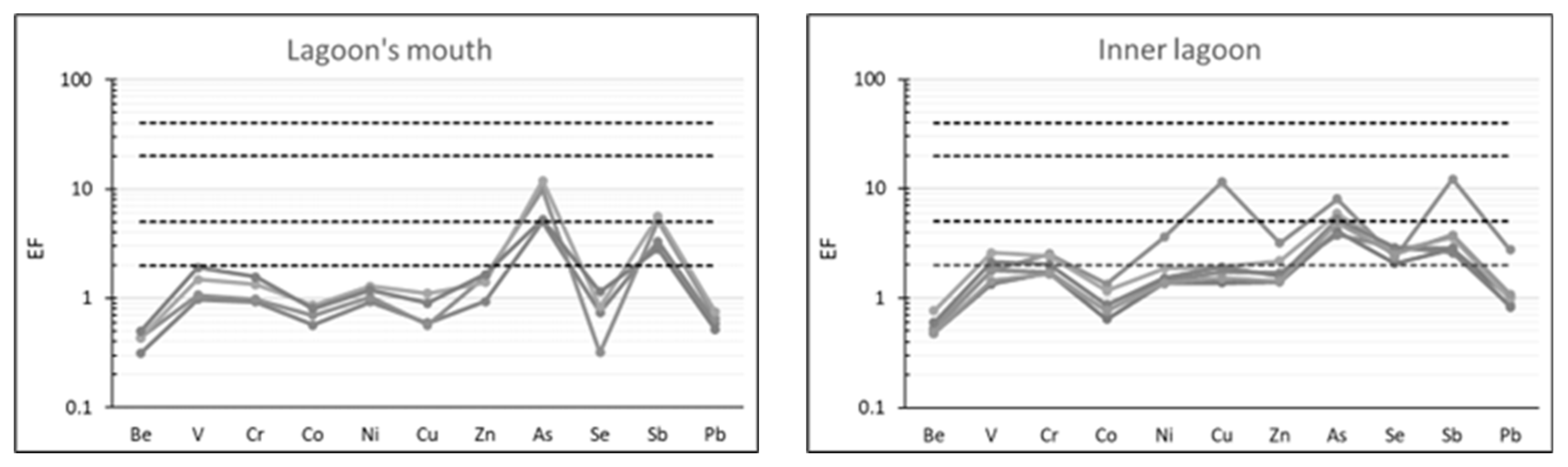
Enrichment Factor (EF): This index is commonly used to speculate on the origin of elements in soils, lake sediments, peat, tailings, and other environmental materials [31]. EF is calculated using the following formula:
EF = (Ci/Cie)s/(Ci/Cie)rs
where Ci represents the concentration of element i in the sample of interest and Cie is the concentration of the immobile element in the sample of interest or in the reference sample. Thus, (Ci/Cie)s is the ratio of the heavy metal to the immobile element in the sample of interest, while the ratio (Ci/Cie)rs is relative to the reference sample [32]. Typically, immobile elements such as Al, Li, Sc, Zr, Ti, Fe, or Mn are considered as reference elements [31]. In this study, Al was used as it is suitable for grain size in most sediment/soil types [31]. As reference values, the upper continental values proposed by Wedepohl (1995) [33,34] were used. Generally, five contamination categories are recognized based on EF: EF < 2—depletion to mineral enrichment; 2 ≤ EF < 5—moderate enrichment; 5 ≤ EF < 20—significant enrichment; 20 ≤ EF < 40—very high enrichment; and EF > 40—extremely high enrichment [35].
-
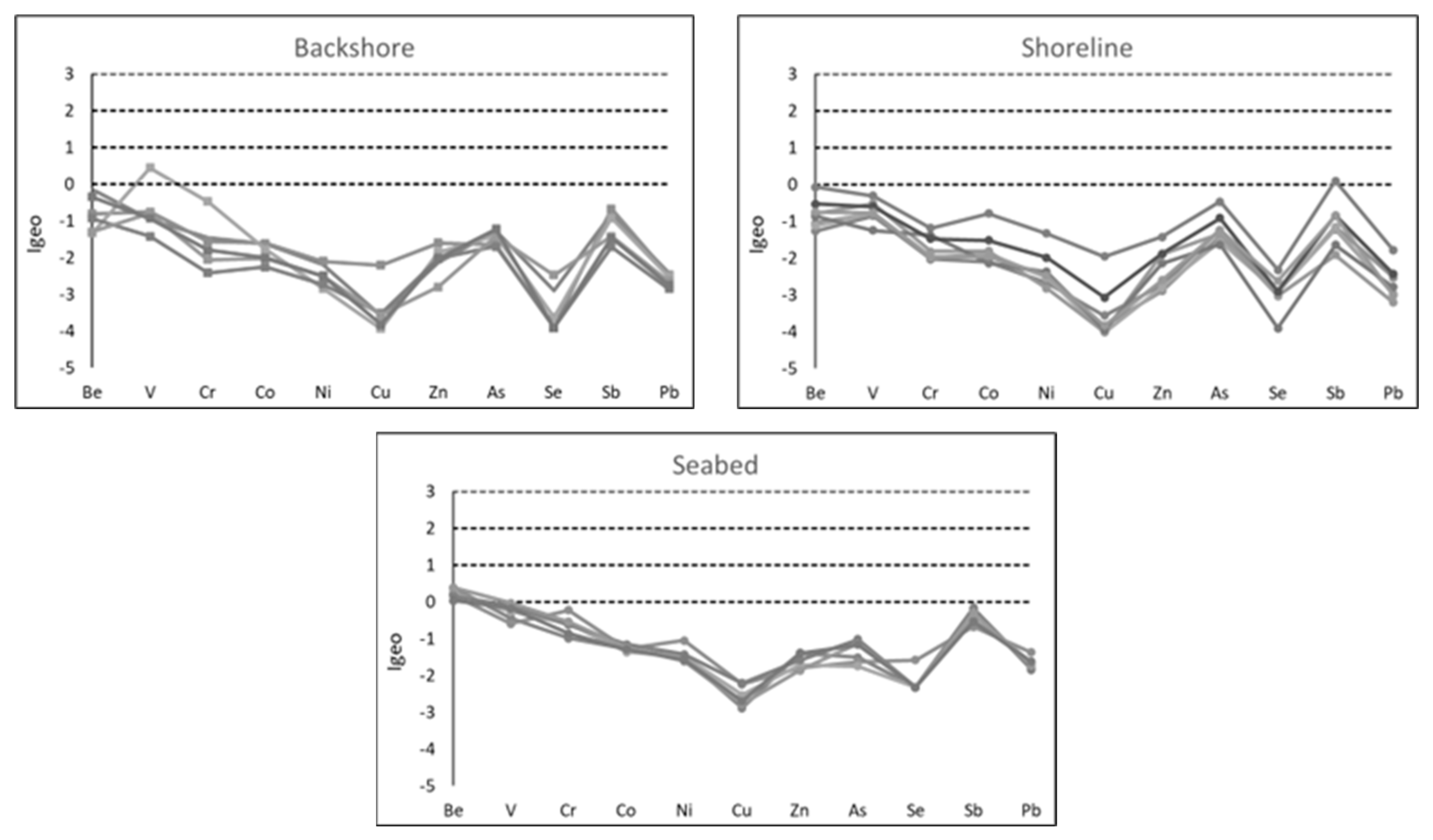
Geoaccumulation Index (Igeo): This index is used to determine and quantify metal contamination in sediments by comparing current concentrations with pre-industrial levels [36]. Igeo is calculated using the following formula:
Igeo = log2[Ci/(1.5Cri)]
where Ci is the concentration of metal i in the sediment, Cri is the background concentration or reference value of metal i, and 1.5 is a correction factor. For this study, the background values used were those of Be, V, Cr, Co, Ni, Cu, Zn, As, Se, Sb, and Pb in deep soils of the northeastern coastal depositional unit in the Veneto region, as defined by the Regional Agency for Environmental Prevention of the Veneto Region [30]. Igeo is generally classified into seven classes: Igeo ≤ 0—unpolluted; 0 < Igeo ≤ 1—unpolluted to moderately polluted; 1 < Igeo ≤ 2—moderately polluted; 2 < Igeo ≤ 3—moderately polluted to strongly polluted; 3 < Igeo ≤ 4—strongly polluted; 4 < Igeo ≤ 5—strongly polluted to extremely polluted; Igeo > 5—extremely polluted [37].
-
Contamination Factor (CF): This index is quantified by the ratio between the concentration of the chemical element under investigation and its pre-industrial concentration in the region under study [38]. This index is calculated by the following equation:
CF = Ci/Cri
where Ci is the concentration of the examined element, and Cri is the pre-industrial concentration of the element. Ideally, Ci should be an average value from at least five sampling sites [39]. For this study, the background values used were those of Be, V, Cr, Co, Ni, Cu, Zn, As, Se, Sb, and Pb in deep soils of the northeastern coastal depositional unit in the Veneto region, as defined by the Regional Agency for Environmental Prevention of the Veneto Region [30]. The CF is generally classified into the following classes: CF < 1—low contamination; 1 ≤ CF ≤ 3—moderate contamination; 3 ≤ CF ≤ 6—considerable contamination; and CF > 6—very high contamination [38,39].
-
Pollution Load Index (PLI): This index is a tool used to evaluate the quality of sediments [40]. This index is calculated by the following equation:
PLI = (CF1 × CF2 × CFn)1/n
where CF1, CF2, and CFn are the Contamination Factors of elements 1, 2, and n, respectively. This index is divided into three categories: PLI > 1—polluted; PLI = 1—baseline levels of pollution; and PLI < 1—not polluted [41,42].

4. Results

4.1. Coastal Samples

4.1.1. Texture Analysis

In the sediment samples collected from the backshore areas, the mean particle size (Mz) ranged between 2.03 Φ and 2.43 Φ, with an average value of 2.26 Φ (fine sands). The percentage abundance of different granulometric fractions within these sediments was, on average, as follows: 20.4% medium sands, 75.8% fine sands, 2.5% very fine sands, and 1.4% mud. These sediments exhibited a well-sorted nature (σ = 0.34 Φ), with values ranging between 0.28 Φ (very well sorted) and 0.58 Φ (moderately sorted). Based on skewness, these sediments demonstrated, on average, a positive asymmetry (Sk = 0.20) with values ranging from 0.13 (positive skewness) to 0.42 (very positive skewness). In terms of kurtosis, the samples ranged between 0.93 (mesokurtic) and 2.15 (very leptokurtic). They showed, on average, a leptokurtic distribution with a K = 1.12 (Table 2).
The samples from the shoreline areas were characterized by a mean particle size (Mz) ranging between 1.92 Φ (medium sands) and 2.34 Φ (fine sands), with an average value of 2.14 Φ. The proportional distribution of distinct granulometric fractions within these sediments was, on average, ascertained as fine sands (60.9%), medium sands (36.9%), very fine sands (1.8%), and a minor fraction of mud (0.3%). The samples were, on average, well sorted (σ = 0.34), with values falling in the range of 0.30–0.38 Φ. These sediments displayed a prevalent positive asymmetry (Sk = 0.13) with values ranging between 0.06 (nearly symmetrical) and 0.17 (positively skewed). Regarding kurtosis, they showed, on average, a mesokurtic distribution (K = 0.98), with values ranging between 0.91 and 1.09 (mesokurtic) (Table 2).
The samples from the seabed areas showed, on average, an Mz of 3.65 Φ (very fine sands), with values ranging from 2.51 Φ (fine sands) to 7.25 Φ (medium-fine silt). The proportional distribution of various granulometric fractions within these sediments included medium sands (4.0%), fine sands (18.8%), very fine sands (51.2%), fine sands (18.8%), silt (17.3%), and clay (8.7%). Regarding sorting, samples showed values that varied between 0.34 Φ (well sorted) and 2.57 Φ (poorly sorted), with an average value of 0.90 Φ (moderately sorted). The skewness values indicated a positive asymmetrical pattern (Sk = 0.30) on average, with values falling in the range of 0.00 (nearly symmetrical) and 0.78 (very positive skewness). In terms of kurtosis, the sediments exhibited a tendency towards leptokurtic distribution on average (K = 1.43), with values that varied between 0.84 (platykurtic) and 3.32 (extremely leptokurtic) (Table 2).

4.1.2. Geochemical Analysis

The calcimetry analyses performed on the backshore samples unveiled notable carbonate contents (Table 3), with a predominance of dolomite (49%) over calcite (40%), resulting in an overall high carbonate content of 89%. A congruous carbonate value of 87.73 wt. % was attained by combining the CaO (33.35 wt. %) and MgO (14.58 wt. %) derived from WD-XRF analysis, along with the volatile content determined through L.O.I. analysis (39.80 wt. %). The remaining oxides exhibited minor proportions, with SiO2 accounting for 9.66 wt. % and Al2O3 for 1.27 wt. %, while the other oxides (Fe2O3, TiO2, MnO, Na2O, K2O, and P2O5) constituted less than 1 wt. % each (Table 4). In terms of heavy metal concentrations, Zn, Cr, and V manifested values falling within the 10–25 ppm range, while Co, Ni, Cu, As, and Pb exhibited concentrations between 1 ppm and 9 ppm. Lastly, Be, Se, Sb, and Tl were present at concentrations below 1 ppm (Table 5).
The samples collected from the shoreline areas exhibited lower carbonate contents (83%) compared to those from the backshore (Table 3), with a calcite content slightly higher (42%) than that of dolomite (40%). The summation of CaO (34.01 wt. %), MgO (13.19 wt. %), and L.O.I. (37.83 wt. %) was also aligned (85.03 wt. %) with the calcimetry results. Regarding other oxides, the SiO2 content was 12.07 wt. %, Al2O3 was 1.48 wt. %, and similarly, the remaining oxides were below 1 wt. % (Table 4). As for heavy metal concentrations, Zn and V exhibited concentrations falling in the range of 10–20 ppm, while Cr, Co, Ni, Cu, As, and Pb displayed concentrations ranging from 1 ppm to 10 ppm. Furthermore, Be, Se, Sb, and Tl showed concentrations below 1 ppm (Table 5).
The samples collected from the seabed areas exhibited the lowest carbonate content (Table 2) in the Bibione coast (74%), wherein the average calcite content (36%) was slightly lower than that of dolomite (37%). The summation of CaO (28.34 wt. %), MgO (12.44 wt. %), and L.O.I. (34.52 wt. %) concurred (75.30 wt. %) with the carbonate content determined through calcimetry. Regarding other oxides, the SiO2 content was the highest in the coastal area (18.61 wt. %), followed by Al2O3 (3.20 wt. %) and Fe2O3 (1.30 wt. %), while the remaining oxides were below 1 wt. % (Table 4). As for heavy metal concentrations, Zn, Cr, and V exhibited concentrations ranging from 19 ppm to 30 ppm; Co, Ni, Cu, As, and Pb displayed concentrations ranging from 3 ppm to 10 ppm. Finally, Be, Se, and Sb showed concentrations below 1 ppm (Table 5).

4.1.3. Pollution Indexes

Regarding the EF, in the backshore samples, the highest values were observed for As and Sb: As was found to be significantly enriched to highly enriched, while Sb was moderately enriched to significantly enriched. The other heavy metals, on the other hand, had EF values below 2 (depletion to mineral enrichment), except for one sample where V and Cr were significantly enriched, and Zn was moderately enriched (Figure 2).
In the shoreline samples, the highest enrichment levels were also observed for As and Sb: As ranged from significantly enriched to highly enriched, while Sb ranged from moderately enriched to significantly enriched. Some cases showed moderate enrichment for V and Zn, while the other metals were not enriched, except for one sample where Ni and Cu showed moderate enrichment (Figure 2).
In the seabed samples, all investigated metals, except for As and Sb, were found to be non-enriched. As ranged from moderately enriched to significantly enriched, while Sb showed moderate enrichment (Figure 2).
Regarding the Igeo values, in the backshore samples, almost all the investigated samples were found to be “unpolluted.” Only one exception was identified in a sample, which was classified as “unpolluted to moderately polluted” for V (Figure 3). Similarly, the shoreline samples were also classified as “unpolluted,” except for a single sample classified as “unpolluted to moderately polluted” for Sb (Figure 3).
As for the seabed samples, they were all classified as “unpolluted to moderately polluted” in terms of Be. For all other investigated metals, these samples were classified as “unpolluted” (Figure 3).
Regarding the CF, the backshore and shoreline samples were found to be non-contaminated for all the investigated heavy metals. However, the seabed samples showed moderate contamination levels for Be, V, and Sb (Figure 4). In terms of PLI, all three environments considered were classified as non-polluted (Figure 4).

4.2. Lagoon Samples

4.2.1. Texture Analysis

In the sediment samples obtained from the lagoon’s mouth, the Mz ranged between 2.21 Φ (fine sands) and 6.07 Φ (medium-fine silt), with an average Mz of 3.41 Φ (very fine sands). The percentage distribution of different granulometric fractions was, on average, as follows: medium sands 16.6%, fine sands 44.7%, very fine sands 8.9%, silt 19.4%, and clay 10.4%. These sediments exhibited an overall poor sorting (σ = 1.61 Φ), with values falling in the range of 0.39 Φ (well sorted) to 3.07 (very poorly sorted). They showed a positive skewness (Sk = 0.39) on average, with values ranging between −0.10 (nearly symmetrical) and 0.74 (very positive skewness). Regarding kurtosis, the samples exhibited a leptokurtic tendency on average (K = 1.12), with values falling in the range of 0.71–2.61 (Table 6).
In the samples from the inner lagoon, the Mz ranged between 5.87 Φ (medium-fine silt) and 8.06 Φ (clay), with an average of 7.13 Φ. The abundance of different grain size fractions, on average, was as follows: medium sand (0.1%), fine sand (3.0%), very fine sand (8.1%), silt (53.9%), and clay (35.0%). In terms of sorting, these sediments exhibited, on average, a very poor sorting (2.53 Φ) with values ranging between 2.25 Φ and 3.07 Φ. Based on the skewness, they displayed a positive asymmetry on average (Sk = 0.23), with values ranging between −0.04 (nearly symmetrical) and 0.36 (very positive skewness). Regarding kurtosis, these samples showed values falling in the range of 0.85–1.03 with an average value of K = 0.91 (platykurtic) (Table 6).

4.2.2. Geochemical Analysis

The results of calcimetry analysis carried out on the samples from the lagoon’s mouth (Table 7) revealed an average carbonate content of 69%, with a higher proportion of calcite (38%) compared to dolomite (31%). The sum of CaO (29.86 wt. %), MgO (10.00 wt. %), and L.O.I. (31.33 wt. %) aligned with the results of the calcimetry (71.19%). In terms of other oxides, the SiO2 content was 23.09 wt. %, Al2O3 was 3.20 wt. %, Fe2O3 was 1.25 wt. %, while the remaining oxides (TiO2, MnO, Na2O, K2O, and P2O5) were below 1 wt. % (Table 8). As for the heavy metal concentrations, Zn, Cr, and V exhibited concentrations within the range of 15–30 ppm. Co, Ni, Cu, As, and Pb displayed concentrations ranging from 3 ppm to 9 ppm. Lastly, Be, Se, Sb, and Tl showed concentrations below 1 ppm (Table 9).
The samples from the inner lagoon, on the other hand, exhibited a lower carbonate content (63%) compared to those from the lagoon’s mouth, with a slight prevalence of dolomite (32%) over calcite (31%). The sum of CaO (24.56 wt. %), MgO (10.50 wt. %), and L.O.I. (31.92 wt. %) agreed (66.98 wt. %) with the results of calcimetry (Table 7). As for the other oxides, the content of SiO2 was 23.51 wt. %, Al2O3 5.44 wt. %, Fe2O3 2.13%, K2O 1.00 wt. %, while the other oxides (TiO2, MnO, Na2O, and P2O5) were below 1 wt. % (Table 8). With respect to the concentration of heavy metals, these samples exhibited the highest levels compared to both the coastal area samples and the lagoon’s mouth samples: the concentrations of V and Zn ranged from 60 ppm to 70 ppm, Cr, Ni, and Cu were in the range of 20–50 ppm; Pb, As, and Co were in the range of 6–14 ppm, while Be and Se were below 1.15 ppm (Table 9).

4.2.3. Pollution Indexes

Regarding the EF, the samples from the lagoon’s mouth showed non-enrichment for almost all the heavy metals considered. The only exceptions were As and Sb, where both showed moderate to significant enrichment (Figure 5).
In the Inner lagoon samples, enrichments were observed for several investigated metals: again, As and Sb showed moderate to significant enrichment; Se showed moderate enrichment in all the samples; and V and Cr exhibited moderate enrichment in two of the investigated samples. It was also evident that one sample had moderate enrichments in V, Cr, Ni, Zn, and Pb and significant enrichments in Cu, As, and Sb (Figure 5).
Regarding the Igeo, the samples from the lagoon’s mouth were found to be “unpolluted” for almost all the investigated heavy metals. The only exceptions were one sample classified as “unpolluted to moderately polluted” for Be and V and two samples classified as “unpolluted to moderately polluted” for Be (Figure 6).
In the samples from the inner lagoon, several samples showed pollution for different heavy metals: all samples were classified as “moderately polluted” for Be; in terms of V, the samples ranged from “unpolluted to moderately polluted” to “moderately polluted”; all samples were classified as “unpolluted to moderately polluted” for Cr; and some samples were classified as “unpolluted to moderately polluted” for Co, Ni, Cu, Zn, Se, and Sb. Additionally, there was one sample classified as “moderately polluted to highly polluted” for Cu, “moderately polluted” for Be, V, and Sb, and “unpolluted to moderately polluted” for Cr, Co, Ni, Zn, and Pb (Figure 6).
Regarding the CF, the sediment samples from the lagoon’s mouth were found to be “moderately contaminated” for Be and V, while they were non-contaminated for all other investigated heavy metals (Figure 7). As for the Inner lagoon, contamination was observed for all the investigated heavy metals except for As; this environment was classified as “considerably contaminated” for Be and V and “moderately contaminated” for Cr, Co, Ni, Cu, Zn, Se, Sb, and Pb (Figure 7). In terms of PLI, the lagoon’s mouth environment was classified as “unpolluted,” while the Inner lagoon environment was classified as “polluted” (Figure 7).

5. Discussion

5.1. Coastal Samples

Regarding the backshore and shoreline samples, it has been observed that, on average, they exhibited a mean grain size (Mz) that characterized them as fine sands, with a certain homogeneity in both environments. However, it was noticeable that, on average, the shoreline samples were slightly coarser than those of the backshore. This could be attributed to the action of incoming and outgoing waves in the shoreline environment, which can remove finer sediments through winnowing processes [18], resulting in a lower Mz in this environment compared to the backshore. This was also reflected in terms of sorting, as the higher energy in the shoreline environment allows for better sediment selection. In fact, although both backshore and shoreline samples were generally well to very well sorted, the range of variability was much narrower in the shoreline samples compared to the others. However, it is important to note that in addition to wave action, other factors, such as currents, tides, winds, and storm events, can influence sediment sorting in the shoreline environment, interacting with each other and creating complex dynamics that shape sediment sorting patterns along the shoreline.
Skewness provides useful information for sediment characterization, measuring the symmetry in the frequency distribution of grain size. Positive skewness values can indicate the dominance of fine sediments or deposition areas, while negative values can indicate the dominance of coarse sediments or erosion areas due to high-energy environments [43]. The comparison between the normal curve and the grain size distribution curve of winnowed sands suggests that the “tail” at the fine end of the sand distribution curve has been “cut”, resulting in a negative skewness [42]. In the case of this study, although negative skewness values were not observed in the shoreline environment, they were generally lower than those in the backshore, which could be attributed to the selective action of waves. The positive skewness values in both the backshore and shoreline environments were in contrast to previous studies in which negative skewness values were observed in modern sandy beaches [44,45,46]. In the context of this work, it was difficult to identify the reasons for this contrast, but several factors that may have influenced this parameter can be considered:
  • The coastal area of Bibione is heavily urbanized and used for tourism purposes, resulting in the presence of several beach resorts and motorized beach cleaning activities, among others. Sampling was carried out in July during the peak of the tourist summer season, and the results of a single campaign do not allow for a qualitative and quantitative assessment of the impact of anthropogenic activities;
  • Over the years, the beaches of Bibione have undergone beach nourishment interventions, especially in the northeastern area;
  • Friedman (1961) [44] demonstrated that river sands generally exhibit positive skewness, and Bibione is located on one of the lobes of the bicuspidate delta formed at the mouth of the Tagliamento River. However, it is difficult to consider the sands of the beaches of Bibione as river sands, as they are exposed to wind and waves, and there is no hydrodynamic influence from the Tagliamento River;
  • Storm events can lead to sediment redistribution, which is also reflected in the skewness parameter. Generally, storm events result in an increase in grain size on the beach due to higher wave energy. However, in extreme cases, the water level can reach the dune system, causing erosion and redistribution of fine sediments that constitute the dunes onto the beach. This leads to a reduction in grain size, which is associated with a shift towards positive skewness values [47]. The Bibione area was impacted approximately nine months before the sampling date, between 27 and 30 October 2018, by an intense extreme storm event. This event, named “Vaia,” brought winds reaching 200 km/h in the Veneto, Friuli, and Trentino inland regions [48], and it caused significant damage along the Venetian coast as well. Weather data from stations in the city of Lignano Sabbiadoro (northeast wing of the Tagliamento River delta) indicated gusts of wind reaching 93 km/h [49]. According to authorities, the effects of the storm resulted in the removal of approximately 100 thousand cubic meters of sand from the beach. However, it remains challenging to attribute the high skewness values observed in all samples from Bibione beaches solely to the effects of the Vaia storm, even though it did impact the dune system. Indeed, dunes are only present in the areas near the mouth of the Baseleghe lagoon and close to the mouth of the Tagliamento River. In the rest of the coast, they were largely depleted during the intensive urbanization period of the 1960s.
The seabed samples exhibited significantly different textural characteristics compared to the beach samples, due to the distinct hydrodynamic conditions characterizing this environment. On average, these samples showed an Mz value classifying them as very fine sands, with some samples falling within the fine sand range and others within the silt range, indicating a lower energy prevailing in this environment. The wide range of Mz values is probably related even to the presence of submerged sand bars close to the shoreline. The sorting of these samples ranged from moderate to very poorly sorted. This is consistent with the findings of previous studies [50,51,52,53], which suggested that medium to fine sands have better sorting, which tends to deteriorate as sediments become finer or coarser. At the mouth area of the Tagliamento River (NE zone), significant differences were observed compared to all other samples (Figure 8): the sediments located right at the river outlet were classified as poorly to very poorly sorted, with a highly positive skewness and a kurtosis ranging from highly leptokurtic to extremely leptokurtic. The highly positive skewness indicates excessive fluvial input [54], while extremely high or low kurtosis values indicate that the sediment has achieved that level of sorting in other environments with higher energy [55].
Regarding the compositional aspects of the investigated samples, it was observed that they were mainly composed of carbonates, with a slight prevalence of dolomite over calcite, in accordance with previous studies [56]. An additional observation was made regarding the carbonate content of samples in the coastal area of Bibione. Despite the high percentage of carbonate in these sediments, a systematic decrease was identified from samples obtained in the backshore environment to those obtained in the seabed environment. Specifically, shoreline sediments showed a carbonate content (83%) that was lower than that of backshore sediments (89%). On the other hand, seabed sediments exhibited an even lower carbonate content (74%). It was observed that the carbonate content showed a high negative correlation with the abundance of very fine sand (Table 10). At the same time, it was noticed that both SiO2 and Al2O3 (Table 10) were positively correlated with the abundance of very fine sand. This suggests that the lower carbonate content in seabed sediments may be due to a higher content of siliciclastic sediments concentrated in the grain size fraction of very fine sands, which dominates this environment (51.2%). However, the aforementioned explanation would not appear applicable to the observed decrease in carbonate content of the shoreline sediments, where the abundance of very fine sands was very low (1.4%).
So, another factor that could be considered for the observed variations is the dissolution processes undergone by the carbonate sediments of the shoreline and seabed due to contact with seawater. For example, the contribution of carbonate chemical dissolution to coastal erosion has been observed in the coastal area of Alicante (Southeast of the Iberian Peninsula) [57]. In the context of this work, there are no data to support this, so a better understanding of whether and to what extent the dissolution affects the observed variations is needed through leaching tests under different temperature, pH, and salinity conditions. If this phenomenon is indeed occurring, it could contribute to the existing problems of coastal erosion in the Bibione coastal area [24]. This becomes particularly relevant considering the acidification processes that could affect the seas due to the increasing atmospheric CO2 concentration [58,59,60] and taking into account the decrease in pH between 1983 and 2008 observed in the northern Adriatic Sea by Lucchetta et al. [61]. The dissolution of carbonates could also contribute to a reduction in sand grain size [57], which could lead to a worsened sediment quality and, consequently, environmental quality in general. In fact, an increase in the content of fine fractions could lead to an increase in the concentration of heavy metals in the sediments, resulting in a deterioration in quality. It is well known in the scientific literature that pollutants such as heavy metals tend to be adsorbed on the surface of finer sediments, particularly in clayey sediments [62,63,64,65]. Furthermore, it has been observed that calcareous clays have a good adsorption capacity for metals such as copper and zinc [66,67].
Regarding the heavy metal concentrations, the calculated EF values on these samples indicated that the coastal environment was enriched in As and Sb, suggesting a possible anthropogenic origin [35,68]. On the other hand, the Igeo and CF indices did not highlight contamination or pollution from As, while contaminations from Sb, along with Be and V, emerged in the seabed environment.
In this regard, the concentrations of heavy metals in the examined samples were compared to the threshold contamination concentrations for sediments in sites used for public, private, and residential green areas, as defined by Italian law [29]. This comparison, as shown in Figure 9 revealed that the concentrations of heavy metals in the coastal sediments were far below the legal limits, indicating the good quality of the sediments in this area at the time of sampling.
To identify similar behaviors associated with possible common sources, the correlation matrix of the investigated heavy metal concentrations was calculated (Table 11). This matrix showed that most of the heavy metals were strongly correlated with each other, indicating a possible common source [68]. The only two metals that showed very few correlations were V (correlated only with Cr) and As (correlated only with Co), indicating a potentially different source [68]. The correlations V-Cr, Be-Cr, Be-Co, Ni-Cr, and Ni-Co were identified by the Regional Agency for Environmental Prevention of the Veneto Region in the soil and subsurface of the northeastern coastal area of Veneto. These relationships were found to be very similar to those observed in units related to the Tagliamento River, from which the material originates [30]. However, there is a lack of correlation between V and Be, as well as between V and Ni, compared to what was observed in the soil and subsurface of the northeastern coastal area of Veneto. So, this could indicate an external source of V. Similarly, even As appears to originate from an external source. Considering that these sediments derive from the Tagliamento River, which, in its course from the source to the mouth, crosses cities and cultivated fields, it is possible to hypothesize that the sources of As and V are of anthropogenic origin. Indeed, these two elements are associated with anthropogenic activities such as the use of pesticides, fertilizers, and the combustion of fossil fuels [69,70,71,72].

5.2. Lagoon Samples

Regarding the textural aspects (Figure 8) of these samples, noticeable differences in grain size were immediately observed between the samples taken from the lagoon’s mouth area and those from the inner area of the lagoon. Specifically, the samples from the lagoon’s mouth area exhibited, on average, a mean grain size (Mz) characteristic of very fine sands, while the samples from the inner area had, on average, an Mz indicative of medium-fine silt. These differences reflected the expected variations in the depositional environments where the sediments were sampled, suggesting that the lagoon’s mouth area represents a higher-energy environment compared to the inner part. These differences were also evident in terms of sorting. Although the entire lagoon area exhibited a low sorting degree, the samples from the innermost part of the lagoon stood out by displaying very poor sorting. This situation was likely due to an excess of fine material in these samples, resulting in a limited degree of sediment sorting, as extensively reported by different authors [50,51,52,53]. This observed pattern can be attributed to the landward decrease in flow velocity, reducing the ability of the current to transport sand from the sea [41]. Conversely, the grain size and compositional characteristics of the samples from the lagoon’s mouth indicated a strong influence of the sea in this area, leading to the transportation of sands to this part of the lagoon. It is well known that coarser sediments have a higher settling velocity, and tidal currents do not possess sufficient strength to transport sands over long distances, resulting in the deposition of sandy sediments closer to the mouth [73,74].
The observed textural differences were also reflected in the compositional characteristics, as the samples from the inner part of the lagoon exhibited a lower carbonate content and higher amounts of SiO2, Al2O3, and K2O. In this context, it was observed that Al2O3 and K2O exhibited a high positive correlation with clay abundance (Table 12). Furthermore, it has also been noted that there is a strong positive correlation between these two oxides (Table 12), suggesting the presence of a higher quantity of clay minerals in these sediments [75,76].
The textural characteristics of the inner part of the lagoon make this environment particularly vulnerable to heavy metal pollution. As previously discussed, heavy metals tend to adsorb onto the surface of finer sediments, especially in clayey fractions [62,63,64,65]. This vulnerability could be further exacerbated if there is indeed a contribution from the dissolution of carbonates, as mentioned earlier, which could lead to an increase in the finer fraction in this area.
Pollution phenomena in the sediments of this part of the lagoon could be potentially problematic from both an environmental and economic standpoint, considering the presence of the tourist port “Porto Baseleghe”. The phenomenon of bottom silting, which can reach levels that inhibit navigation and require dredging interventions, is one of the main issues in port management. The dredged sediments must have high chemical and ecotoxicological quality to be reused in other contexts. If the sediments are of poor quality, they must be treated or disposed of in landfills, resulting in significant increases in management costs for port activities [7].
The calculated EF values on these samples indicated that even the lagoon environment was enriched in As and Sb. In addition to these, in the inner lagoon portion, there were some samples moderately enriched in V and Cr, suggesting a possible anthropogenic origin [35,68]. The Igeo and CF indices highlighted that some samples from the lagoon’s mouth exhibited pollution from V and Cr. On the other hand, the inner part of the lagoon showed pollution from all the investigated heavy metals, particularly from Be, V, and Cr.
The concentrations of heavy metals in the examined samples were compared to the threshold contamination concentrations for sediments in sites used for public, private, and residential green areas, as defined by Italian law [29]. This comparison (Figure 10) revealed that the concentrations of heavy metals in the coastal sediments were far below the legal limits, indicating the good quality of the sediments in this area at the time of sampling. It also showed that, although the samples from the inner part of the lagoon exhibited the highest concentration values in the entire area, there were no critical situations at the time of sampling, neither in the lagoon’s mouth area nor in the more vulnerable inner part.
The correlation matrix of heavy metal concentrations was also calculated for the samples from the lagoon area, and it showed that most of the investigated heavy metals were correlated with each other (Table 13). This result is consistent with the previous findings regarding the correlations between heavy metals in the soil and subsoil of the northeastern coastal area of Veneto [30]: the strong correlations between V-Cr, V-Be, V-Cr, Be-Cr, Be-Co, Ni-Cr, and Ni-Co can be mainly associated with the material originating from the sediment (transported by the Tagliamento River). This could suggest that the observed situation in terms of heavy metal enrichment is likely due to the geomorphological, sedimentological, and hydrodynamical characteristics of the lagoon. The correlations between Sb, Cu, Zn, As, and Pb could be related to an anthropogenic source, such as the presence of the tourist port in the lagoon, since they are typical contaminants associated with port activities [77,78].
In light of what has been observed, the lagoon area seems to confirm its vulnerability to heavy metal pollution, as seen in other contexts [8,9,10,11]. In terms of port management, monitoring the quality of sediments would allow for the timely detection of critical pollution situations. This would enable proactive measures to be taken to mitigate potential environmental impacts. Such monitoring would be deemed necessary to ensure the continued protection of the ecosystem and to prevent any potential risks to human health and the environment, which would also have potentially impacting consequences on the economies of the tourist port.

6. Conclusions

The findings of this study highlighted significant differences in sediment characteristics between the backshore, shoreline, and seabed environments due to the complex interplay between hydrodynamics, depositional processes, and anthropogenic influences.
The shoreline samples exhibited slightly coarser sediments compared to those of the backshore, indicating the selective removal of finer sediments by incoming and outgoing waves. The higher energy in the shoreline environment allows for more effective sediment selection, resulting in a more homogeneous and well-sorted sediment composition.
In contrast to previous studies, positive skewness values were observed in both the backshore and shoreline environments. This departure from the expected negative skewness may be connected to the influence of other factors: the coastal area of Bibione, characterized by heavy urbanization and tourism, may experience disturbances from beach resorts and motorized beach cleaning activities, together with beach nourishment activities, potentially impacting sediment characteristics. Through this study, based on a single sampling campaign, it was not possible to quantify the impact of human activities on the characteristics of the sediments. Furthermore, the observed skewness values could also be associated with the severe storm “Vaia,” which occurred in October 2018.
The seabed samples displayed distinct textural characteristics, with a mean grain size classifying them as very fine sands. The low energy prevailing in this environment allows for the deposition of finer sediments, resulting in moderate to very poorly sorted samples. Also evident were the differences, especially in terms of sorting, skewness, and kurtosis, of the samples taken at the mouth of the Tagliamento River. Overall, it can be hypothesized that the role of hydrodynamic conditions, geomorphological features, grain size, and fluvial input influenced the textural characteristics and sorting patterns of seabed samples.
Regarding the compositional aspects, carbonates were found to be the dominant component in all investigated samples, with dolomite slightly prevailing over calcite. However, a systematic decrease in carbonate content was observed from the backshore to the seabed samples. This could be partially explained by the increase in very fine sand in the seabed sediments, resulting in a higher content of siliciclastic material. However, this explanation cannot be applied to the shoreline environment, where there is a very low content of very fine sand. So, another factor that could be considered for the observed variations is the dissolution processes undergone by the carbonate sediments of the shoreline and seabed due to contact with seawater. Further investigations, including leaching tests under various conditions, are necessary to understand the extent and implications of carbonate dissolution on coastal erosion and sediment quality, especially considering the acidification processes of the seas connected to climate change. In conclusion, one can emphasize the importance of the need to investigate dissolution processes, coastal erosion, changes in ocean chemistry, sediment quality, and pollutant adsorption capacity as co-factors involved in the observed changes and consider their potential impacts on coastal environments. The differences in grain size and composition observed in the lagoon samples reflected the contrasting depositional environments within the lagoon system. The lagoon’s mouth area, influenced by the proximity to the sea, exhibited coarser sediments, likely due to higher-energy conditions, which was also associated with a slightly better degree of sorting than the internal part. In contrast, the inner part of the lagoon displayed a lower sorting degree and a greater presence of finer sediments, indicative of reduced flow velocity and limited sediment transport. These variations highlight the importance of local hydrodynamic conditions in shaping sediment characteristics and make the inner part of the lagoon particularly vulnerable to heavy metal pollution, as fine sediments have a greater propensity for adsorbing pollutants. In this context, although the different pollution indexes indicated the presence of pollution in both the coastal area (Sb, Be, and V) and the lagoon area (V, Cr, and Be), the concentrations were below the limits set by Italian law. These observations underscore the need to monitor and manage heavy metal pollution in the lagoon system, especially in the context of environmental protection and the management of the tourist port located within the lagoon. It would seem, however, that the concentrations of some elements (V and As in the coastal area; Pb, Zn, Cu, Sb, and As in the lagoon) could be connected to anthropogenic sources. This highlights the importance of identifying and addressing anthropogenic activities that contribute to heavy metal pollution in the lagoon system. Understanding the sources of pollution is crucial for effective management and mitigation strategies.
In conclusion, the monitoring of the sediment quality in the Bibione coastal area, particularly in the Baseleghe Lagoon, is essential for environmental protection and for the management of the tourist port located within the lagoon; maintaining good sediment quality would reduce the costs associated with dredging interventions. This emphasizes the economic and environmental benefits of preserving sediment quality and its implications for sustainable management practices. Understanding these factors is crucial for effective environmental management, pollution mitigation, and the preservation of the lagoon ecosystem.
To conclude, maintaining good sediment quality can help bring about several economic and environmental benefits: (i) Coastal protection: Sediments play a crucial role in coastal protection by acting as a natural buffer against erosion and storm surge. Sediment deposits, such as beaches and dunes, provide a protective barrier that helps absorb wave energy and mitigate the impacts of coastal storms. By maintaining good sediment quality, the stability and resilience of coastlines can be preserved, reducing the need for costly artificial interventions like seawalls or beach replenishment projects. (ii) Navigation and shipping: Sediment quality impacts navigation in harbors, ports, and shipping channels. Accumulation of excessive sediments, such as silt or fine grains, can impede vessel movement, causing navigational hazards and reducing the efficiency of shipping operations. Regular monitoring and management of sediment quality can help ensure safe and efficient navigation, reducing the need for costly dredging operations and potential disruptions to maritime trade. (iii) Tourism and recreation: Sediment quality plays a significant role in attracting tourists and supporting recreational activities in coastal areas. Pristine sandy beaches, clear waters, and healthy coastal ecosystems are major attractions for tourists seeking beach holidays, water sports, and other recreational activities. Maintaining good sediment quality contributes to the aesthetic appeal and ecological health of coastal destinations, bolstering tourism revenues and supporting local economies. (iv) Ecosystem health and biodiversity: Sediments are essential components of coastal ecosystems, supporting a diverse array of flora and fauna. Healthy sediment quality provides suitable habitats for various species, including important marine organisms, shellfish beds, and seagrass meadows. By maintaining good sediment quality, the ecological balance and biodiversity of coastal ecosystems can be preserved, ensuring the sustainability of fisheries, supporting recreational fishing activities, and protecting sensitive habitats. (v) Water quality and nutrient cycling: sediments play a vital role in nutrient cycling and water quality regulation. They act as sinks and sources of nutrients, helping to maintain the balance and availability of essential elements for aquatic life. Good sediment quality can enhance water clarity, reduce the risks of harmful algal blooms, and improve overall water quality conditions. This is particularly important for sustaining healthy aquatic ecosystems, supporting fisheries, and preserving the recreational value of coastal waters.
Ultimately, by recognizing the economic and environmental benefits associated with maintaining good sediment quality, coastal managers can implement appropriate monitoring programs, conservation measures, and sustainable management strategies. These efforts will contribute to the long-term well-being of coastal communities, promote ecosystem resilience, and ensure the sustainable use of coastal resources.

Author Contributions

Conceptualization, A.A., E.M. and C.V.; methodology, A.A., E.M., U.T. and C.V.; validation, A.A., E.M., M.G.P. and U.T.; formal analysis, A.A., E.M., M.G.P. and U.T.; investigation, A.A., E.M., U.T. and C.V.; resources, U.T. and C.V.; data curation, A.A., E.M. and M.G.P.; writing—original draft preparation, A.A., E.M. and U.T.; writing—review and editing, A.A., E.M., M.G.P., U.T. and C.V.; visualization, A.A., E.M. and U.T.; supervision, E.M. and C.V.; project administration, E.M. and C.V.; funding acquisition, C.V. All authors have read and agreed to the published version of the manuscript.

Funding

The data presented in this manuscript have been collected in the framework of the EU INTERREG ITALY-CROATIA CBC PROGRAMME 2014–2020 ECOMAP (ECOsustainable Management of MArine and tourist Ports)—CUP F76C18000630005.

Data Availability Statement

Raw data that support the findings of this study are made available on request.

Acknowledgments

The authors thank Renzo Tassinari of the Department of Physics and Earth Sciences of the University of Ferrara for his important help in carrying out the WD-XRF and ICP-MS analysis of sediments.

Conflicts of Interest

The authors declare no conflict of interest.

References

  1. Neumann, B.; Vafeidis, A.T.; Zimmermann, J.; Nicholls, R.J. Future Coastal Population Growth and Exposure to Sea-Level Rise and Coastal Flooding—A Global Assessment. PLoS ONE 2015, 10, e0131375. [Google Scholar] [CrossRef]
  2. Lotze, H.K.; Lenihan, H.S.; Bourque, B.J.; Bradbury, R.H.; Cooke, R.G.; Kay, M.C.; Kidwell, S.M.; Kirby, M.X.; Peterson, C.H.; Jackson, J.B.C.; et al. Depletion, Degradation, and Recovery Potential of Estuaries and Coastal Seas. Science 2006, 312, 1806–1809. [Google Scholar] [CrossRef] [PubMed]
  3. He, Q.; Silliman, B.R. Climate Change, Human Impacts, and Coastal Ecosystems in the Anthropocene. Curr. Biol. 2019, 29, R1021–R1035. [Google Scholar] [CrossRef]
  4. He, Q.; Bertness, M.D.; Bruno, J.F.; Li, B.; Chen, G.; Coverdale, T.C.; Altieri, A.H.; Bai, J.; Sun, T.; Pennings, S.C.; et al. Economic Development and Coastal Ecosystem Change in China. Sci. Rep. 2014, 4, 5995. [Google Scholar] [CrossRef] [PubMed]
  5. Pérez-Ruzafa, A.; Marcos, C.; Pérez-Ruzafa, I.M. Mediterranean Coastal Lagoons in an Ecosystem and Aquatic Resources Management Context. Phys. Chem. Earth Parts A/B/C 2011, 36, 160–166. [Google Scholar] [CrossRef]
  6. Tagliapietra, D.; Sigovini, M.; Ghirardini, A.V. A Review of Terms and Definitions to Categorise Estuaries, Lagoons and Associated Environments. Mar. Freshw. Res. 2009, 60, 497. [Google Scholar] [CrossRef]
  7. Bosa, S.; Petti, M.; Pascolo, S. Improvement in the Sediment Management of a Lagoon Harbor: The Case of Marano Lagunare, Italy. Water 2021, 13, 3074. [Google Scholar] [CrossRef]
  8. El Ouaty, O.; El M’rini, A.; Nachite, D.; Marrocchino, E.; Marin, E.; Rodella, I. Assessment of the Heavy Metal Sources and Concentrations in the Nador Lagoon Sediment, Northeast-Morocco. Ocean Coast. Manag. 2022, 216, 105900. [Google Scholar] [CrossRef]
  9. Glasby, G.; Szefer, P.; Geldon, J.; Warzocha, J. Heavy-Metal Pollution of Sediments from Szczecin Lagoon and the Gdansk Basin, Poland. Sci. Total Environ. 2004, 330, 249–269. [Google Scholar] [CrossRef]
  10. Youssef, M.; El-Sorogy, A. Environmental Assessment of Heavy Metal Contamination in Bottom Sediments of Al-Kharrar Lagoon, Rabigh, Red Sea, Saudi Arabia. Arab. J. Geosci. 2016, 9, 474. [Google Scholar] [CrossRef]
  11. Shetaia, S.A.; Abu Khatita, A.M.; Abdelhafez, N.A.; Shaker, I.M.; El Kafrawy, S.B. Human-Induced Sediment Degradation of Burullus Lagoon, Nile Delta, Egypt: Heavy Metals Pollution Status and Potential Ecological Risk. Mar. Pollut. Bull. 2022, 178, 113566. [Google Scholar] [CrossRef]
  12. European Parliament. Directive 2008/56/EC of the European Parliament and of the Council—Establishing a Framework for Community Action in the Field of Marine Environmental Policy (Marine Strategy Framework Directive). Off. J. Eur. Parliament. 2008, 26, 136–157. [Google Scholar]
  13. European Commission. Report from the Commission to the European Parliament and to the Council on the Implementation of the Marine Strategy Framework Directive (Directive 2008/56/EC); COM(2020) 259 Final; European Commission: Brussels, Belgium, 2020; p. 34. [Google Scholar]
  14. European Commission. Communication from the Commission—The European Green Deal; COM(2019) 640 final; European Commission: Brussels, Belgium, 2019; p. 24. [Google Scholar]
  15. Castellarin, A.; Nicolich, R.; Fantoni, R.; Cantelli, L.; Sella, M.; Selli, L. Structure of the Lithosphere beneath the Eastern Alps (Southern Sector of the TRANSALP Transect). Tectonophysics 2006, 414, 259–282. [Google Scholar] [CrossRef]
  16. Fontana, A. L’evoluzione Geomorfologica Della Bassa Pianura Friulana e Le Sue Relazioni Con Le Dinamiche Insediative Antiche. In Monografie del Museo Friulano di Storia Naturale; Museo Friulano di Storia Naturale: Udine, Italy, 2006; Volume 46. [Google Scholar]
  17. Fontana, A.; Mozzi, P.; Bondesan, A. Late Pleistocene Evolution of the Venetian–Friulian Plain. Rend. Fis. Acc. Lincei 2010, 21, 181–196. [Google Scholar] [CrossRef]
  18. Bondesan, A.; Meneghel, M. Geomorfologia Della Provincia Di Venezia; Bondesan, A., Meneghel, M., Eds.; ESEDRA: Padova, Italy, 2004; p. 195.217. [Google Scholar]
  19. Marocco, R. Evoluzione Quaternaria Della Laguna Di Marano (Friuli Venezia Giulia). Il Quat. 1989, 2, 125–137. [Google Scholar]
  20. Marocco, R. Evoluzione Tardopleistocenica-Olocenica Del Delta Del F. Tagliamento E Delle Lagune Di Marano E Grado (Golf. Di Trieste). Il Quat. 1989, 4, 223–232. [Google Scholar]
  21. Rosato, P.; Stellin, G. A Multi-Criteria Approach to Territorial Management: The Case of the Caorle and Bibione Lagoon Nature Park. Agric. Syst. 1993, 41, 399–417. [Google Scholar] [CrossRef]
  22. Poulain, P.M. Tidal Currents in the Adriatic as Measured by Surface Drifters: ADRIATIC TIDAL CURRENTS. J. Geophys. Res. Ocean. 2013, 118, 1434–1444. [Google Scholar] [CrossRef]
  23. Fontolan, G.; Bezzi, A.; Pillon, S. Rischio Di Mareggiata. In Atlante Geologico della Provincia di Venezia. Cartografie e Note illustrative; Vitturi, A., Ed.; Provincia di Venezia: Venice, Italy, 2011; pp. 581–600. [Google Scholar]
  24. Regione del Veneto—Ufficio di Statistica Regione del Veneto. Tourist Movement in the Veneto Region (Consultation by Resort-Annual and Monthly Data). Available online: https://statistica.regione.veneto.it/banche_dati_economia_turismo_turismo1.jsp (accessed on 7 July 2023).
  25. Krumbein, W.C. Size Frequency Distributions of Sediments. SEPM JSR 1934, 4, 65–77. [Google Scholar] [CrossRef]
  26. Folk, R.L.; Ward, W.C. Brazos River Bar [Texas]; a Study in the Significance of Grain Size Parameters. J. Sediment. Res. 1957, 27, 3–26. [Google Scholar] [CrossRef]
  27. Wentworth, C.K. A Scale of Grade and Class Terms for Clastic Sediments. J. Geol. 1922, 30, 377–392. [Google Scholar] [CrossRef]
  28. Legislative Decree 152/06 Annex 5, Part VI, Table 1. Soil and Subsoil Contamination Thresholds. In Sites for Public, Private and Residential Green Use; Government of the Italian Republic: Rome, Italy, 2006.
  29. AA.VV. Technical Directorate—Veneto Soil and Reclamation Center Service. In Metals and Metalloids in the Veneto Soils—Definition of Background Values, 2019th ed.; Regional Agency for Environmental Prevention of the Veneto Region (ARPAV): Veneto, Italy, 2019; p. 190. [Google Scholar]
  30. Reimann, C.; De Caritat, P. Distinguishing between Natural and Anthropogenic Sources for Elements in the Environment: Regional Geochemical Surveys versus Enrichment Factors. Sci. Total Environ. 2005, 337, 91–107. [Google Scholar] [CrossRef] [PubMed]
  31. Zhang, L.; Ye, X.; Feng, H.; Jing, Y.; Ouyang, T.; Yu, X.; Liang, R.; Gao, C.; Chen, W. Heavy Metal Contamination in Western Xiamen Bay Sediments and Its Vicinity, China. Mar. Pollut. Bull. 2007, 54, 974–982. [Google Scholar] [CrossRef] [PubMed]
  32. Dung, T.T.T.; Cappuyns, V.; Swennen, R.; Phung, N.K. From Geochemical Background Determination to Pollution Assessment of Heavy Metals in Sediments and Soils. Rev. Environ. Sci. Biotechnol. 2013, 12, 335–353. [Google Scholar] [CrossRef]
  33. Hans Wedepohl, K. The Composition of the Continental Crust. Geochim. Cosmochim. Acta 1995, 59, 1217–1232. [Google Scholar] [CrossRef]
  34. Sutherland, R.A. Bed Sediment-Associated Trace Metals in an Urban Stream, Oahu, Hawaii. Environ. Geol. 2000, 39, 611–627. [Google Scholar] [CrossRef]
  35. Banat, K.M.; Howari, F.M.; Al-Hamad, A.A. Heavy Metals in Urban Soils of Central Jordan: Should We Worry about Their Environmental Risks? Environ. Res. 2005, 97, 258–273. [Google Scholar] [CrossRef]
  36. Buccolieri, A.; Buccolieri, G.; Cardellicchio, N.; Dell’Atti, A.; Di Leo, A.; Maci, A. Heavy Metals in Marine Sediments of Taranto Gulf (Ionian Sea, Southern Italy). Mar. Chem. 2006, 99, 227–235. [Google Scholar] [CrossRef]
  37. Hakanson, L. An Ecological Risk Index for Aquatic Pollution Control. A Sedimentol. Approach. Water Res. 1980, 14, 975–1001. [Google Scholar] [CrossRef]
  38. Loska, K.; Wiechuła, D.; Korus, I. Metal Contamination of Farming Soils Affected by Industry. Environ. Int. 2004, 30, 159–165. [Google Scholar] [CrossRef]
  39. Tomlinson, D.L.; Wilson, J.G.; Harris, C.R.; Jeffrey, D.W. Problems in the Assessment of Heavy-Metal Levels in Estuaries and the Formation of a Pollution Index. Helgol. Meeresunters 1980, 33, 566–575. [Google Scholar] [CrossRef]
  40. Ferreira, S.L.C.; Da Silva, J.B.; Dos Santos, I.F.; De Oliveira, O.M.C.; Cerda, V.; Queiroz, A.F.S. Use of Pollution Indices and Ecological Risk in the Assessment of Contamination from Chemical Elements in Soils and Sediments—Practical Aspects. Trends Environ. Anal. Chem. 2022, 35, e00169. [Google Scholar] [CrossRef]
  41. Friedman, G.M. Distinction Between Dune, Beach, and River Sands from Their Textural Characteristics. SEPM JSR 1961, 31, 514–529. [Google Scholar] [CrossRef]
  42. Duane, D.B. Significance of Skewness in Recent Sediments, Ester Pamlico Sound, North Carolina. J. Sediment. Petrol. 1964, 34, 864–874. [Google Scholar] [CrossRef]
  43. Friedman, G.M. Dynamic Processes and Statistical Parameters Compared for Size Frequency Distribution of Beach and River Sands. SEPM JSR 1967, 37, 327–354. [Google Scholar] [CrossRef]
  44. Friedman, G.M. Address of the Retiring President of the International Association of Sedimentologists: Differences in Size Distributions of Populations of Particles among Sands of Various Origins. Sedimentology 1979, 26, 3–32. [Google Scholar] [CrossRef]
  45. Chappel, J. Recognizing Fossil Strand Lines From Grain-Size Analysis. SEPM JSR 1967, 37. [Google Scholar] [CrossRef]
  46. Siegle, E.; Calliari, L.J. High-Energy Events and Short-Terms Changes in Superficial Beach Sediments. Braz. J. Ocanography 2009, 56, 149–152. [Google Scholar] [CrossRef]
  47. Rizzolo, R.; Giudice, L.D.; Jahdi, R.; Salis, M. Assessing the Potential Impacts of the Vaia Storm on Wildfire Spread and Behavior in the Veneto Region. In ICFBR 2022; MDPI: Basel, Switzerland, 2022; p. 1. [Google Scholar] [CrossRef]
  48. Regional Agency for Environmental Prevention of Friuli Venezia-Giulia Region. Archivio-dati. meteo.fvg. Available online: https://www.meteo.fvg.it/archivio.php?ln=&p=dati (accessed on 21 July 2023).
  49. Hough, J.L. Sediments of Cape Cod Bay, Massachusetts. SEPM JSR 1942, 12. [Google Scholar] [CrossRef]
  50. Inman, D.L. Sorting of Sediments in the Light of Fluid Mechanics. SEPM JSR 1949, 19. [Google Scholar] [CrossRef]
  51. Griffiths, J.C. Size versus Sorting in Some Caribbean Sediments. J. Geol. 1951, 59, 211–243. [Google Scholar] [CrossRef]
  52. Inman, D.L.; Chamberlain, T.K. Particle-Size Distribution in Nearshore Sediments. In Finding Ancient Shorelines; SEPM Society for Sedimentary Geology: Claremore, OK, USA, 1955. [Google Scholar] [CrossRef]
  53. Angusamy, N.; Rajamanickam, G.V. Depositional Environment of Sediments along the Southern Coast of Tamil Nadu, India. Oceanologia 2006, 48, 87–102. [Google Scholar]
  54. Ramanathan, A.L.; Rajkunar, K.; Majumdar, J.; Singh, G.; Behera, P.N.; Santra, S.C.; Chidambaran, S. Textural Characteristics of the Surface Sediments of a Tropical Mangrove Sunbardan Ecosystem India. Indian J. Mar. Sci. 2009, 38, 297–403. [Google Scholar]
  55. Gazzi, P.; Zuffa, G.G.; Paganelli, L.; Gandolfi, G. Provenienza e Dispersione Litoranea Delle Sabbie Delle Spiagge Adriatiche Fra Le Foci Dell’Isonzo e Del Foglia: Inquadramento Regionale. In Memorie della Società Geologica Italiana; Springer: Berlin/Heidelberg, Germany, 1973; No. 12; pp. 1–37. [Google Scholar]
  56. López, I.; López, M.; Aragonés, L.; García-Barba, J.; López, M.P.; Sánchez, I. The Erosion of the Beaches on the Coast of Alicante: Study of the Mechanisms of Weathering by Accelerated Laboratory Tests. Sci. Total Environ. 2016, 566–567, 191–204. [Google Scholar] [CrossRef]
  57. Doney, S.C.; Fabry, V.J.; Feely, R.A.; Kleypas, J.A. Ocean Acidification: The Other CO2 Problem. Annu. Rev. Mar. Sci. 2009, 1, 169–192. [Google Scholar] [CrossRef] [PubMed]
  58. Turley, C.; Findlay, H.S. Ocean Acidification. In Climate Change; Elsevier: Amsterdam, The Netherlands, 2016; pp. 271–293. [Google Scholar] [CrossRef]
  59. Naviaux, J.D.; Subhas, A.V.; Rollins, N.E.; Dong, S.; Berelson, W.M.; Adkins, J.F. Temperature Dependence of Calcite Dissolution Kinetics in Seawater. Geochim. Cosmochim. Acta 2019, 246, 363–384. [Google Scholar] [CrossRef]
  60. Luchetta, A.; Cantoni, C.; Catalano, G. New Observations of CO2-Induced Acidification in the Northern Adriatic Sea over the Last Quarter Century. Chem. Ecol. 2010, 26, 1–17. [Google Scholar] [CrossRef]
  61. Thorne, L.T.; Nickless, G. The Relation between Heavy Metals and Particle Size Fractions within the Severn Estuary (U.K.) Inter-tidal Sediments. Sci. Total Environ. 1981, 19, 207–213. [Google Scholar] [CrossRef]
  62. Sakai, H.; Kojima, Y.; Saito, K. Distribution of Heavy Metals in Water and Sieved Sediments in the Toyohira River. Water Res. 1986, 20, 559–567. [Google Scholar] [CrossRef]
  63. Davies, C.A.L.; Tomlinson, K.; Stephenson, T. Heavy Metals in River Tees Estuary Sediments. Environ. Technol. 1991, 12, 961–972. [Google Scholar] [CrossRef]
  64. Wakida, F.T.; Lara-Ruiz, D.; Temores-Peña, J.; Rodriguez-Ventura, J.G.; Diaz, C.; Garcia-Flores, E. Heavy Metals in Sediments of the Tecate River, Mexico. Environ. Geol 2008, 54, 637–642. [Google Scholar] [CrossRef]
  65. Musso, T.B.; Parolo, M.E.; Pettinari, G.; Francisca, F.M. Cu (II) and Zn (II) Adsorption Capacity of Three Different Clay Liner Materials. J. Environ. Manag. 2014, 146, 50–58. [Google Scholar] [CrossRef] [PubMed]
  66. Sdiri, A.T.; Higashi, T.; Jamoussi, F. Adsorption of Copper and Zinc onto Natural Clay in Single and Binary Systems. Int. J. Environ. Sci. Technol. 2014, 11, 1081–1092. [Google Scholar] [CrossRef]
  67. Zhuang, Q.; Li, G.; Liu, Z. Distribution, Source and Pollution Level of Heavy Metals in River Sediments from South China. CATENA 2018, 170, 386–396. [Google Scholar] [CrossRef]
  68. Imtiaz, M.; Rizwan, M.S.; Xiong, S.; Li, H.; Ashraf, M.; Shahzad, S.M.; Shahzad, M.; Rizwan, M.; Tu, S. Vanadium, Recent Advancements and Research Prospects: A Review. Environ. Int. 2015, 80, 79–88. [Google Scholar] [CrossRef]
  69. Matschullat, J. Arsenic in the Geosphere—A Review. Sci. Total Environ. 2000, 249, 297–312. [Google Scholar] [CrossRef]
  70. Cheng, Q.; Zhou, W.; Zhang, J.; Shi, L.; Xie, Y.; Li, X. Spatial Variations of Arsenic and Heavy Metal Pollutants before and after the Water-Sediment Regulation in the Wetland Sediments of the Yellow River Estuary, China. Mar. Pollut. Bull. 2019, 145, 138–147. [Google Scholar] [CrossRef]
  71. Liaghati, T.; Preda, M.; Cox, M. Heavy Metal Distribution and Controlling Factors within Coastal Plain Sediments, Bells Creek Catchment, Southeast Queensland, Australia. Environ. Int. 2004, 29, 935–948. [Google Scholar] [CrossRef]
  72. Wang, Y.; Gao, S.; Hebbeln, D.; Winter, C. Modeling Grain Size Distribution Patterns in the Backbarrier Tidal Basins, East Frisian Wadden Sea (Southern North Sea). J. Coast. Res. 2011, 64, 850–854. [Google Scholar]
  73. Rouse, H. Engineering Hydraulics Proceedeings of Fourth Hydraulics Conference, Iowa Institute of Hydraulic Research, 12–15 June 1949; Wiley: New York, NY, USA, 1950. [Google Scholar]
  74. Carniello, L.; Defina, A.; D’Alpaos, L. Modeling Sand-Mud Transport Induced by Tidal Currents and Wind Waves in Shallow Microtidal Basins: Application to the Venice Lagoon (Italy). Estuar. Coast. Shelf Sci. 2012, 102, 105–115. [Google Scholar] [CrossRef]
  75. Nair, V.; Achyuthan, H. Geochemistry of Vellayani Lake Sediments: Indicators of Weathering and Provenance. J. Geol. Soc. India 2017, 89, 21–26. [Google Scholar] [CrossRef]
  76. Sinha, S.; Ghosh, S.K.; Kumar, R.; Sangode, S.J. Geochemistry of Neogene Siwalik Mudstones along Punjab Re-Entrant, India: Implications for Source-Area Weathering, Provenance and Tectonic Setting. Curr. Sci. 2007, 92, 1103–1113. [Google Scholar]
  77. Araújo, D.F.; Ponzevera, E.; Briant, N.; Knoery, J.; Bruzac, S.; Sireau, T.; Brach-Papa, C. Copper, Zinc and Lead Isotope Signatures of Sediments from a Mediterranean Coastal Bay Impacted by Naval Activities and Urban Sources. Appl. Geochem. 2019, 111, 104440. [Google Scholar] [CrossRef]
  78. Filella, M.; Belzile, N.; Chen, Y.-W. Antimony in the Environment: A Review Focused on Natural Waters. Earth-Sci. Rev. 2002, 57, 125–176. [Google Scholar] [CrossRef]
Figure 1. Sampling sites in the Bibione coastal area. Coordinates WGS 84/ UTM 32 N; EPSG: 32632.
Jmse 11 01650 g001
Figure 2. EF values in the coastal sediment samples. The dashed black lines represent the various classes for dividing EF values.
Jmse 11 01650 g002
Figure 3. Igeo values in the coastal sediment samples. The dashed black lines represent the various classes for dividing Igeo values.
Jmse 11 01650 g003
Figure 4. In the left graph, the CF values in the backshore, shoreline, and seabed environments are depicted. The dashed lines represent the different classes for dividing CF values. In the right graph, the PLI values in the same environments are presented.
Jmse 11 01650 g004
Figure 5. EF values in the lagoon samples. The dashed black lines represent the various classes for dividing EF values.
Jmse 11 01650 g005
Figure 6. Igeo values in the coastal sediment samples. The dashed black lines represent the various classes for dividing Igeo values.
Jmse 11 01650 g006
Figure 7. In the left graph, the CF values in the backshore, shoreline, and seabed environments are depicted. The dashed lines represent the different classes for dividing CF values. In the right graph, the PLI values in the same environments are presented.
Jmse 11 01650 g007
Figure 8. Distribution of texture statistical parameters (mean grain size, sorting, skewness, and kurtosis) in the analyzed samples.
Jmse 11 01650 g008aJmse 11 01650 g008b
Figure 9. Normalized values of heavy metal concentrations determined in samples from the Bibione coast, with respect to heavy metal contamination threshold concentrations required by Italian law [29].
Jmse 11 01650 g009
Figure 10. Normalized values of heavy metal concentrations determined in samples from the Bibione coast, with respect to heavy metal contamination threshold concentrations required by Italian law [29].
Jmse 11 01650 g010
Table 1. Average (±SD) chemical–physical parameters of the water measured during the sampling campaign.
Measure
Depth (m)
Dissolved Oxygen (mg/L)pHTemperature (°C)Pressure (mbar)Specific
Conductivity (mS/cm)
Absolute
Conductivity (mS/cmA)
Salinity
(ppt)
Seabed37.6 ± 1.28.4 ± 0.024.4 ± 0.51023 ± 138.9 ± 1.338.5 ± 1.624.7 ± 0.9
Max 8.68.424.9102441.741.626.7
Min 4.88.323.2102137.236.623.6
Lagoon’s mouth23.1 ± 1.78.2 ± 0.024.5 ± 0.21005 ± 137.8 ± 8.436.4 ± 7.221.3 ± 4.7
Max 4.58.224.7100647.842.827.5
Min 0.88.224.1100425.425.015.5
Inner Lagoon24.7 ± 3.88.4 ± 0.124.3 ± 0.71015 ±1235.3 ± 5.234.8 ± 4.622.3 ± 3.6
Max 7.48.424.8102439.038.124.8
Min 2.08.323.8100631.731.519.7
Table 2. Average (±SD) values of mean particle size (Mz), sorting (σ), skewness (Sk), and kurtosis (K) in the backshore, shoreline, and seabed samples.
Statistics
Parameter
BackshoreShorelineSeabed
Mz (Φ)2.26 ± 0.122.14 ± 0.113.65 ± 1.05
Max2.432.347.25
Min2.031.922.51
σ (Φ)0.34 ± 0.080.34 ± 0.030.90 ± 0.74
Max0.580.382.57
Min0.280.300.34
Sk0.20 ± 0.070.13 ± 0.030.30 ± 0.25
Max0.410.170.78
Min0.130.060.00
K1.12 ± 0.330.98 ± 0.051.43 ± 0.72
Max2.151.093.32
Min0.930.910.84
Table 3. Mean (±SD) carbonate content (total carbonate, calcite, and dolomite) in coastal samples.
Carbonate Content
(%)
BackshoreShorelineSeabed
Total Carbonate89 ± 583 ± 474 ± 7
Max979090
Min817266
Calcite40 ± 542 ± 336 ± 5
Max484747
Min323728
Dolomite49 ± 640 ± 637 ± 4
Max654746
Min402531
Table 4. Mean (±SD) major oxide composition in coastal samples.
Oxide Composition
(wt. %)
BackshoreShorelineSeabed
SiO29.66 ± 3.5612.07 ± 2.7018.61 ± 1.77
TiO20.11 ± 0.060.07 ± 0.010.22 ± 0.03
Al2O1.27 ± 0.431.48 ± 0.333.44 ± 0.54
Fe2O30.83 ± 0.100.84 ± 0.091.30 ± 0.14
MnO0.02 ± 0.000.02 ± 0.000.03 ± 0.00
MgO14.58 ± 1.6813.19 ± 1.0212.44 ± 0.93
CaO33.35 ± 0.5934.01 ± 0.6128.34 ± 1.50
Na2O0.18 ± 0.070.23 ± 0.060.45 ± 0.04
K2O0.17 ± 0.080.21 ± 0.070.60 ± 0.10
P2O50.04 ± 0.010.04 ± 0.000.06 ± 0.01
L.O.I.39.80 ± 2.2837.83 ± 2.0134.52 ± 0.72
Table 5. Mean (±SD) heavy metal concentrations in coastal sediments.
Heavy Metal Concentration
(ppm)
BackshoreShorelineSeabed
Be0.25 ± 0.080.25 ± 0.070.50 ± 0.04
Max
Min
0.38
0.17
0.40
0.17
0.55
0.43
V22 ± 1120 ± 428 ± 4
Max
Min
45
12
27
14
32
22
Cr10.7 ± 5.29.3 ± 2.119.5 ± 3.3
Max
Min
21.6
5.6
13.1
7.3
25.6
15.1
Co2.1 ± 0.32.3 ± 0.83.1 ± 0.1
Max
Min
2.45
1.57
4.3
1.7
3.4
2.9
Ni4.1 ± 0.84.7 ± 1.78.3 ± 1.2
Max
Min
5.25
3.14
8.9
3.2
10.8
7.4
Cu2.3 ± 1.22.2 ± 1.43.9 ± 0.7
Max
Min
4.86
1.47
5.8
1.4
4.9
3.0
Zn16.9 ± 3.914.9 ± 5.423 ± 3
Max
Min
22.7
9.9
25.6
9.3
26
19
As5.2 ± 0.66.2 ± 1.75.5 ± 1.0
Max
Min
5.97
4.32
10.0
4.5
6.9
4.1
Se0.01 ± 0.010.02 ± 0.010.03 ± 0.01
Max
Min
0.03
0.01
0.03
0.01
0.05
0.03
Sb0.33 ± 0.090.37 ± 0.170.56 ± 0.07
Max
Min
0.45
0.22
0.77
0.19
0.64
0.45
Pb2.7 ± 0.32.6 ± 0.95.2 ± 0.4
Max
Min
3.1
2.3
4.7
1.8
6.3
4.6
Table 6. Average (±SD) values of mean particle size (Mz), sorting (σ), skewness (Sk), and kurtosis (K) in the samples from lagoon’s mouth and inner lagoon.
Statistics
Parameters
Lagoon’s MouthInner Lagoon
Mz (Φ)3.41 ± 1.377.13 ± 0.68
Max6.078.06
Min2.215.87
σ (Φ)1.52 ± 0.962.53 ± 0.23
Max3.073.07
Min0.392.25
Sk0.39 ± 0.320.23 ± 0.10
Max0.740.36
Min−0.10−0.04
K1.61 ± 0.790.91 ± 0.05
Max2.611.03
Min0.710.85
Table 7. Mean (±SD) carbonate content (total carbonate, calcite, and dolomite) in lagoon samples.
Mean Carbonate Content
(%)
Lagoon’s MouthInner Lagoon
Total Carbonate69 ± 963 ± 9
Max8480
Min6055
Calcite38 ± 431 ± 5
Max4441
Min3223
Dolomite31 ± 632 ± 5
Max4039
Min2324
Table 8. Mean (±SD) major oxide composition in lagoon samples.
Oxide Composition
(wt. %)
Lagoon’s MouthInner Lagoon
SiO223.09 ± 3.8523.51 ± 2.68
TiO20.15 ± 0.030.27 ± 0.03
Al2O3.20 ± 0.665.44 ± 1.11
Fe2O31.25 ± 0.132.13 ± 0.54
MnO0.02 ± 0.000.03 ± 0.00
MgO10.00 ± 0.8210.50 ± 1.02
CaO29.86 ± 2.0424.56 ± 2.98
Na2O0.49 ± 0.080.53 ± 0.12
K2O0.56 ± 0.121.00 ± 0.23
P2O50.07 ± 0.010.12 ± 0.03
L.O.I.31.33 ± 2.4031.92 ± 0.81
Table 9. Mean (±SD) heavy metal concentrations in lagoon samples.
Heavy Metal Concentration
(ppm)
Lagoon’s MouthInner Lagoon
Be0.50 ± 0.141.13 ± 0.18
Max
Min
0.77
0.37
1.45
0.91
V29 ± 1167 ± 11
Max
Min
50
22
85
47
Cr16.0 ± 647 ± 6
Max
Min
27.1
10.7
55
37
Co3.3 ± 0.76.7 ± 1.3
Max
Min
4.6
2.5
9.6
5.5
Ni7.8 ± 221.6 ± 7.4
Max
Min
11.0
5.5
41.2
15.9
Cu4.0 ± 126 ± 27
Max
Min
6.4
2.1
101
16
Zn26 ± 1063 ± 17
Max
Min
42
14
101
46
As6.1 ± 1.27.5 ± 1.0
Max
Min
7.5
4.98
9.9
5.4
Se0.03 ± 0.010.16 ± 0.04
Max
Min
0.05
0.01
0.22
0.10
Sb0.49 ± 0.070.91 ± 0.51
Max
Min
0.60
0.4
2.33
0.51
Pb4.0 ± 0.613.5 ± 5.8
Max
Min
4.9
3.1
28.9
7.7
Table 10. Correlation indices of total carbonate content, SiO2 content, and Al2O3 content versus different granulometric fractions’ abundance. Bold values represent correlation coefficients with a p-value < 0.05.
Total CarbonateSiO2Al2O3
SiO2−0.96
Al2O3−0.920.93
Medium Sand0.32−0.35−0.53
Fine Sand0.68−0.80−0.85
Very Fine Sand−0.770.760.89
Mud−0.040.670.79
Table 11. Correlation matrix between heavy metal concentrations in the coastal sediments. Bold values represent correlation coefficients with a p-value < 0.05.
BeVCrCoNiCuZnAsSeSb
Be
V0.24
Cr0.610.70
Co0.720.460.55
Ni0.830.230.690.84
Cu0.550.210.450.830.83
Zn0.580.410.420.740.620.67
As0.170.26−0.010.650.280.390.33
Se0.680.210.600.650.840.570.280.16
Sb0.750.490.560.940.800.800.750.520.54
Pb0.850.390.790.790.950.730.610.170.840.77
Table 12. Correlation indices between SiO2, Al2O3, and K2O versus different granulometric classes’ abundance. Bold values represent correlation coefficients with a p-value < 0.05.
Medium SandFine SandVery Fine SandSiltClaySiO2Al2O3
SiO2−0.30−0.40−0.470.440.58
Al2O3−0.68−0.71−0.360.790.890.85
K2O−0.64−0.71−0.390.780.890.861.00
Table 13. Correlation matrix between heavy metal concentrations in the coastal sediments. Bold values represent correlation coefficients with a p-value < 0.05.
BeVCrCoNiCuZnAsSeSb
Be
V0.97
Cr0.950.92
Co0.840.840.95
Ni0.650.630.850.95
Cu0.300.320.580.770.92
Zn0.760.750.900.980.970.83
As0.270.240.470.590.720.780.66
Se0.960.930.930.830.660.330.750.29
Sb0.200.200.490.690.870.990.770.800.24
Pb0.520.480.760.860.980.940.910.750.550.92
Disclaimer/Publisher’s Note: The statements, opinions and data contained in all publications are solely those of the individual author(s) and contributor(s) and not of MDPI and/or the editor(s). MDPI and/or the editor(s) disclaim responsibility for any injury to people or property resulting from any ideas, methods, instructions or products referred to in the content.

