Port Call Optimization at a Ferry Terminal with Stochastic Servicing Time and Additional Visits

Abstract

Ferry shipping is an indispensable method of public transportation, especially in areas with well-developed river systems or coastal areas. The increasing demand for transport requires additional visits and introduces the problem of ship visit schedule engineering at ferry terminals with stochastic servicing time. In this paper, we propose a ferry visit planning problem to maximize the total profit, in which the berthing time, berthing location, and servicing time for each ferry visit are optimized. Then, a mixed-integer nonlinear programming model is proposed to formulate the focal problem. We propose a tailored solution method to convert the mixed-integer nonlinear programming model to a mixed-integer linear programming model. We further devise an inserting algorithm to test the performance of our model. A comparison between the results of the basic instance yielded by our model and those of the inserting algorithm validates our model and solution method. We then conduct sensitivity analyses of the impacts of different numbers of existing ferry visits and added ferry visits, different expectations of the real time taken by all the ferry visits, and different distribution patterns of existing ferry visits, to further validate the performance of our model.

1. Introduction

Ferry shipping is an important component of public transportation servicing and plays an essential role in providing mobility for passengers in cities with coastal areas and river systems, such as Hong Kong [1] and Sydney [2]. In the management of ferry transportation, arranging ferry visits at the ferry terminal is a critical issue that potentially influences the service level and total profit of the ferry operation company. In practice, ferry servicing companies generally arrange ferry visits to provide the servicing for the ferry passengers at the ferry terminal. Specifically, a ferry visit denotes the process of a ferry arriving at the terminal, mooring at a berth, and servicing the disembarking and boarding passengers. The arrangement for ferry visits, including berthing time (ferry arrival times at the port), berthing locations (the berths that ferries moor at), and servicing time (time taken for disembarking and boarding), are generally stipulated in advance by the ferry visit plan, which is designed at the planning stage.

The servicing time of ferry visits is mainly affected by the numbers of boarding and disembarking passengers on each ferry visit. In practice, the number of passengers on each ferry visit is uncertain, which will result in the stochastic servicing time of ferry visits. This is due to the exact value of the passenger demand being unknown at the planning stage, and the servicing time of ferry visits is, thus, stochastic. The ferry servicing company allocates the servicing time for each ferry visit based on the historical passenger demand, which is referred to as allocated servicing time in this paper. The number of passengers taking the ferry will be revealed when the servicing is finished. Then, the actual servicing time of ferry visits will also be acquired. Figure 1 illustrates the ferry visit plan of three ferry visits at two berths, which is designed at the planning stage. Additionally, the actual servicing time of three ferry visits at the operational stage is also revealed in Figure 1. The x-axis and y-axis represent the time and berth, respectively. The actual servicing time and allocated servicing time are denoted by the solid red arrow line and the black one. For ferry visit 1, its actual servicing time (i.e., 25 min) far exceeds the allocated servicing time (i.e., 15 min). Then, ferry visit 2 cannot moor at berth 1 at its designed berthing time and serve passengers on time, thereby affecting the implementation of the ferry visit plan and reducing the servicing quality. For ferry visit 3, its actual servicing time (i.e., 20 min) is less than the allocated servicing time (i.e., 25 min), which will not affect the performance of the ferry servicing system. Therefore, the uncertain servicing time is an essential factor to consider at the planning stage since considering the servicing time uncertainty can make the ferry visit plan more applicable in practical operations.

In addition, the ferry passenger demand varies throughout the day. The ferry passenger demand during the peak hours tends to be higher than that during the flat hours. Correspondingly, the ferry visits operating during the peak hour typically serve more passengers and therefore bring higher revenue to the ferry servicing company. This varying revenue incurred by the time-dependent passenger demand is referred to as the time-dependent revenue in this study.

However, the existing literature does not cover the visit plan optimization problem at ferry terminals with stochastic servicing time and additional visits. To fill the research gap, this paper designs the ferry visit plan from the perspective of the ferry servicing company. Specifically, based on the current plan, we consider redesigning the ferry visit plan to accommodate the newly added ferry visits. The deviation of the redesigned ferry visit plan from the current one is constrained to reduce the impacts on the travel plans of passengers. In addition, this paper also introduces the uncertain servicing time and the time-dependent revenue caused by the characteristics of passenger demand. The berthing time, berthing location, and servicing time for each ferry visit are jointly optimized to maximize the profit of the ferry servicing company. The model originally proposed in this paper will yield the visit plan that maximizes the total profit. Hopefully, this study can provide help ferry companies in optimizing ferry visits at the terminal while facing the increasing transport demand. The main contributions of this paper are as follows:

(1)

This paper studies a ferry visit planning problem to optimize the berthing time, berthing locations, and servicing time for ferry visits simultaneously. In particular, deviation from the current plan, uncertain servicing time, and time-dependent revenue are taken into account. To the best of our knowledge, this is the first time the proposed problem has been studied.

(2)

A mixed-integer nonlinear programming (MINLP) model is proposed to formulate the investigated problem. To solve the model, we apply a linearization method to reformulate the MINLP model to a solvable mixed-integer linear programming (MILP) model. An inserting algorithm is developed to demonstrate the superiority of our model.

(3)

Numerical experiments are conducted using the Hong Kong ferry terminal as an example to validate the applicability of the proposed model. The experimental results demonstrate that our model is effective under various scenarios.

The remainder of this study is organized as follows. Section 2 presents a review of the literature related to this paper. Section 3 provides a description of the investigated problem and the nonlinear mixed-integer programming model. Section 4 shows the solution method, in which we convert the mixed-integer nonlinear programming model to a mixed-integer linear programming model. In Section 5, we summarize the computational experiments, including the basic instance and sensitivity analysis. Finally, Section 6 concludes the paper.

2. Literature Review

Currently, there is only a fraction of papers focusing on the management problems regarding the ferry servicing. Among these works, the ferry network design problem (FNDP), which optimizes the ferry servicing network and passenger flow, is extensively studied. The FNDP was first proposed by [3]. They focused on a multiple origin–destination network flow problem with ferry capacity constraint. In [4], they extended [3] by introducing different ferry servicing types and passenger preferences with arrival time windows. Later, Ref. [5] studied a stochastic FNDP under uncertain demand and formulated a two-stage stochastic model. As an extension of the earlier works, Ref. [6] involved user equilibrium flows and hard capacity constraints. In [7], they proposed two robust optimization models for their FNDP. Recently, Ref. [8] utilized the maximum passenger utility spanning tree approach to optimize the connection between all pairs of ferry stations and the locations of hubs. In [9], they considered FNDP by introducing autonomous ferries. A two-step optimization approach was proposed to identify the optimal autonomous ferry servicing schedules. In their later study, Ref. [10], they focused on planning the ferry servicing schedule, which combined the dial-a-ride on-demand servicing and fixed schedule servicings simultaneously.

Although there has been some ferry-servicing-related research, the ferry visit planning problem that determines the berthing time, berthing location, and servicing time has rarely been studied. Our ferry visit planning problem relates closely to the berth allocation problem (BAP), which allocates the berthing time and locations to the arriving vessels. In the past two decades, many researchers and practitioners have made great efforts to solve the BAP arising in the container port terminal. An early study was proposed by [11], and they focused on the objective of minimizing the overall staying time of vessels and dissatisfaction with vessel berthing order in the BAP. Later, some researchers studied the deterministic BAP by incorporating practical characteristics. For example, Ref. [12] investigated the integration of BAP, quay crane assignment problem, and yard allocation problem. In [13], they also studied an integrated problem that combined BAP with the quay crane allocation and scheduling problems. In practice, it is generally impossible for all the parameters to be fixed and known in advance. Uncertainties often arise in practical operations due to weather conditions and mechanical failures. A comprehensive review of the BAP under uncertainties was given by [14]. According to the review, uncertain factors regarding the arrival time [15,16,17,18], handling time [19,20,21,22], quay crane breakdown [23,24,25], and unscheduled vessel calling [26,27] were commonly considered in BAP problems. Arrival time and handling time are the most common uncertain parameters to be considered in the BAP. For the uncertain arrival time, Ref. [28] introduced a time buffer to handle the uncertain arrival time in the robust BAP. In [29], they proposed a robust model to optimize the berth allocation and quay crane assignment considering arrival time uncertainty. In [30], they addressed a berth allocation and assignment problem under uncertain vessel arrival time and port servicing time, where the cooperation among the liner carriers and that between port operator and liner shipping carriers were involved. For the uncertain handling time, Refs. [31,32] used the robust optimization method and distributionally robust optimization method to solve BAP, respectively. There are also many scholars who considered the uncertainties of arrival time and handling time simultaneously. In [22], they focused on the weekly berth and quay crane planning, where the berth position, berthing time, and quay crane assignment were optimized. In [33], they integrated BAP with yard space allocation, where the uncertain handling time was incurred by the uncertain number of loading and unloading containers. In [34], they optimized the berth allocation, assignment of tugboats, and the vessel sequence at the seaport.

To sum up, most of the existing literature has focused on either FNDP regarding the ferry servicing or BAP targeting the vessels transferring cargoes in the container port terminal. There is no paper studying the ferry visit planning problem that considers the deviation between the redesigned ferry visit plan and the current one, uncertain servicing time, and time-dependent revenue simultaneously. Firstly, the ferry passengers typically prefer the current ferry visit plan. If the redesigned ferry visit plan deviates from the current one, passengers’ travel plans will be affected. Hence, the deviation between the redesigned ferry visit plan and the current one should be considered. Secondly, the passenger demand is uncertain, resulting in an uncertain servicing time. Considering the servicing time uncertainty will make the ferry visit plan more applicable in practical operations. Thirdly, the passenger demand varies throughout the day, which introduces time-dependent revenue. With the consideration of these three practical aspects, our paper can provide the ferry operation company with a more reasonable ferry visits plan, helping it realize the maximum profit.

3. Model Formulation

3.1. Problem Description

At a ferry terminal with multiple identical berths, denoted by $\mathcal{P}$, a group of ferry visits, denoted by ${\mathcal{V}}^{\mathrm{E}}$, is scheduled according to a daily ferry visit plan, which gives the berthing time, berth location, and servicing time for each visit. With the increasing passenger demand, the ferry servicing company plans to add more voyages. The new set of visits $\mathcal{V}$ includes ${\mathcal{V}}^{\mathrm{E}}$ and the visits brought by the added voyages that are denoted by ${\mathcal{V}}^{\mathrm{A}}$. Consequently, the ferry visit plan needs to be redesigned. For management convenience, the operating hours of the ferry terminal are evenly divided into a set of time slots, denoted by $\mathcal{S}$, by time points uniformly distributed, denoted by $\mathcal{T}$. Each time slot $s\in \mathcal{S}$ starts with the time point $t=s$ and ends with time point $t=s+1$. The berth allocation decisions are mainly represented by a series of binary decision variables, namely, ${\pi }_{ij}$ indicating whether visit i is allocated to berth j, ${\xi }_{it}^{\mathrm{B}}$/${\xi }_{it}^{\mathrm{E}}$ indicating whether the allocated berthing time of visit i starts/ends at time point t, and ${\xi }_{is}^{\mathrm{O}}$ indicating whether time slot s is occupied by visit i, $i\in \mathcal{V},j\in \mathcal{P},t\in \mathcal{T},s\in \mathcal{S}$. In light of the traveling time preference of ferry passengers, the benefit of a visit is related to the start berthing time point, denoted by $r_t,t\in \mathcal{T}$. Due to the stochastic number of passengers, the real berthing time of visit $i\in \mathcal{V}$ is uncertain, denoted by ${\tilde{d}}_i$, and we assume that it obeys the normal distribution with the expectation ${\mu }_i$ and the standard deviation ${\sigma }_i$. To handle the servicing time uncertainty, we set the upper limit of the probability that the actual servicing time of a visit exceeds the time slots allocated to it, denoted by $Pro$. Meanwhile, a penalty of $Pe{n}^{\mathrm{EX}}$ will be incurred when such a case happens (EX means time required for the disembarking and boarding of a visit exceeds the allocated time slot). In addition, given that the customers are used to the original visit plan, changes in the berth plan of existing visits $i\in \mathcal{V}$, including the berthing time and berth location, lead to penalties, denoted by $Pe{n}^{\mathrm{ST}}$ (ST means changing the berthing start time of a ferry visit) and $Pe{n}^{\mathrm{BA}}$ (BA means changing the berth allocation of a ferry visit), respectively.

3.2. Mathematical Model

Given the above notations, the ferry visit plan optimization problem can be formulated as follows.

$$\begin{array}{cc}\hfill \left[\mathbf{M}\mathbf{1}\right]& max\sum _{i\in \mathcal{V}}\sum _{t\in \mathcal{T}}{r}_t{\xi }_{it}^{\mathrm{B}}-\sum _{i=1,\dots ,V^{\mathrm{E}}}\sum _{j\in \mathcal{P}}Pe{n}^{\mathrm{BA}}{\overline{\pi }}_{ij}({\overline{\pi }}_{ij}-{\pi }_{ij})-\sum _{i=1,\dots ,V^{\mathrm{E}}}\sum _{t\in \mathcal{T}}Pe{n}^{\mathrm{ST}}{\overline{\xi }}_{it}^{\mathrm{B}}({\overline{\xi }}_{it}^{\mathrm{B}}-{\xi }_{it}^{\mathrm{B}})\hfill \\ \hfill & -\sum _{i\in \mathcal{V}}Pe{n}^{\mathrm{EX}}\mathbb{P}({\tilde{d}}_i\ge \sum _{s\in \mathcal{S}}c{\xi }_{is}^{\mathrm{O}})\hfill \end{array}$$

(1)

subject to

$$\begin{array}{c}\sum _{j\in \mathcal{P}}{\pi }_{ij}=1,\forall i\in \mathcal{V}\end{array}$$

(2)

$$\begin{array}{c}\sum _{t\in \mathcal{T}}{\xi }_{it}^{\mathrm{B}}=1,\forall i\in \mathcal{V}\end{array}$$

(3)

$$\begin{array}{c}\sum _{t\in \mathcal{T}}{\xi }_{it}^{\mathrm{E}}=1,\forall i\in \mathcal{V}\end{array}$$

(4)

$$\begin{array}{c}\sum _{i\in \mathcal{V}}{\pi }_{ij}{\xi }_{is}^{\mathrm{O}}\le 1,\forall j\in \mathcal{P},\forall s\in \mathcal{S}\end{array}$$

(5)

$$\begin{array}{c}{\xi }_{is}^{\mathrm{O}}=\sum _{t=1,\dots ,s}{\xi }_{it}^{\mathrm{B}}-\sum _{t=1,\dots ,s+1}{\xi }_{it}^{\mathrm{E}},\forall s\in \mathcal{S},\forall i\in \mathcal{V}\end{array}$$

(6)

$$\begin{array}{c}\mathbb{P}({\tilde{d}}_i\ge \sum _{s\in \mathcal{S}}c{\xi }_{is}^{\mathrm{O}})\le Pro,\forall i\in \mathcal{V}\end{array}$$

(7)

$$\begin{array}{c}{\pi }_{ij},{\xi }_{it}^{\mathrm{B}},{\xi }_{it}^{\mathrm{E}},{\xi }_{is}^{\mathrm{O}}=0,1,\forall i\in \mathcal{V},\forall j\in \mathcal{P},\forall t\in \mathcal{T},\forall s\in \mathcal{S}.\end{array}$$

(8)

The objective function (1) maximizes the total profit, which equals the benefit of all visits, minus the penalty incurred for changing berth allocation and berthing time, minus the penalty incurred for exceeding the allocated time slots. Constraints (2) ensure that each visit can be assigned to exactly one berth. Constraints (3) and (4) indicate the uniqueness of each visit’s start and end time points. Combined together, constraints (2)–(4) ensure that all visits will be accepted and avoid the waste of berth space by preventing allocating more than one berth to a single visit. Constraints (5) guarantee that each berth can be occupied by at most one visit at any time slot. Constraints (6) indicate that the corresponding visit occupies all time slots between the start and end time points. Constraints (5) and (6) ensure that all visits can stay at the allocated berth from the start of berthing time to the end of berthing time. Constraints (7) restrict that, for each visit, the probability that the real servicing time required exceeds the allocated time slots is no higher than the predetermined upper bound, which guarantees the lower bound of the service level. Constraints (8) are the domains of decision variables.

4. Solution Algorithm

The original model [M1] contains multiple nonlinear elements, including the stochastic parameter and products of decision variables. In this section, we show how to handle them. First, we linearize the products of binary decision variables in (5). To perform this, we introduce a new auxiliary variable.

Then, constraints (5) can be replaced by the following constraints:

$$\begin{array}{c}\sum _{i\in \mathcal{V}}{\varphi }_{ijs}\le 1,\forall j\in \mathcal{P},\forall s\in \mathcal{S}\end{array}$$

(9)

$$\begin{array}{c}{\varphi }_{ijs}\le {\pi }_{ij},\forall i\in \mathcal{V},\forall j\in \mathcal{P},\forall s\in \mathcal{S}\end{array}$$

(10)

$$\begin{array}{c}{\varphi }_{ijs}\le {\xi }_{is}^{\mathrm{O}},\forall i\in \mathcal{V},\forall j\in \mathcal{P},\forall s\in \mathcal{S}\end{array}$$

(11)

$$\begin{array}{c}{\varphi }_{ijs}\ge {\pi }_{ij}+{\xi }_{is}^{\mathrm{O}}-1,\forall i\in \mathcal{V},\forall j\in \mathcal{P},\forall s\in \mathcal{S}.\end{array}$$

(12)

Constraints (9) are the rewritten constraints (5), and constraints (10)–(12) guarantee that the relationship between the variables ${\pi }_{ij}$ and ${\xi }_{is}^{\mathrm{O}}$ remains unchanged.

Next, we tackle the nonlinear element due to the stochastic servicing time ${\tilde{d}}_i$. Since the operating hours are discretized into time slots, and the cumulative distribution functions of ${\tilde{d}}_i\sim \mathcal{N}({\mu }_i,{\sigma }_i^2)$ can be easily obtained, denoted as $F_i\left(x\right)$, we can enumerate all the possible values of ${\sum }_{s\in \mathcal{S}}c{\xi }_{is}^{\mathrm{O}}$ that satisfy $\mathbb{P}({\tilde{d}}_i\ge {\sum }_{s\in \mathcal{S}}c{\xi }_{is}^{\mathrm{O}})\le Pro$, $i\in \mathcal{V}$ and rewrite the objective function (1). Therefore, the stochastic elements in [M1] can be handled with new parameters and variables.

The parameters $Pr{o}_{iu}$ and ${\underline{q}}_i$ are obtained on the characteristics of the cumulative distribution functions $F_i\left(x\right)$ of ${\tilde{d}}_i\sim \mathcal{N}({\mu }_i,{\sigma }_i^2)$, and the time slot length c.

Then, constraints (7) can be replaced by

$$\sum _{s\in \mathcal{S}}{\xi }_{is}^{\mathrm{O}}\ge {\underline{q}}_i,\forall i\in \mathcal{V},$$

(13)

which is a linear constraint that can be directly programmed in a commercial solver.

Meanwhile, the objective function (1) can be rewritten as

$$\begin{array}{cc}\hfill \left[\mathbf{M}\mathbf{2}\right]& max\sum _{i\in \mathcal{V}}\sum _{t\in \mathcal{T}}{r}_t{\xi }_{it}^{\mathrm{B}}-\sum _{i=1,\dots ,V^{\mathrm{E}}}\sum _{j\in \mathcal{P}}Pe{n}^{\mathrm{BA}}{\overline{\pi }}_{ij}({\overline{\pi }}_{ij}-{\pi }_{ij})-\sum _{i=1,\dots ,V^{\mathrm{E}}}\sum _{t\in \mathcal{T}}Pe{n}^{\mathrm{ST}}{\overline{\xi }}_{it}^{\mathrm{B}}({\overline{\xi }}_{it}^{\mathrm{B}}-{\xi }_{it}^{\mathrm{B}})\hfill \\ \hfill & -\sum _{i\in \mathcal{V}}Pe{n}^{\mathrm{EX}}\sum _{u=1,\dots ,\left|\mathcal{S}\right|}Pr{o}_{iu}{\tau }_{iu}\hfill \end{array}$$

(14)

with constraints (2)–(4), constraint (6), constraint (8), constraints (9)–(13), and the following constraints added:

$$\begin{array}{c}\sum _{u=1,\dots ,\left|\mathcal{S}\right|}u{\tau }_{iu}=\sum _{s\in \mathcal{S}}{\xi }_{is}^{\mathrm{O}},\forall i\in \mathcal{V}\end{array}$$

(15)

$$\begin{array}{c}\sum _{u=1,\dots ,\left|\mathcal{S}\right|}{\tau }_{iu}=1,\forall i\in \mathcal{V}.\end{array}$$

(16)

The probability of the real servicing time exceeding the allocated time slot, $\mathbb{P}({\tilde{d}}_i\ge {\sum }_{s\in \mathcal{S}}c{\xi }_{is}^{\mathrm{O}})$ can be rewritten as the probability of real servicing time exceeding the total length of the allocated time slots. Constraints (15) and (16) calculate the total number of time slots allocated to each visit. As a result, the original model [M1] is linearized as [M2], which can be solved by an off-the-shelf commercial solver Gurobi 10.0 by Gurobi Optimization, Beaverton, OR, USA.

5. Numerical Examples

The solution method was programmed in Pycharm with Python interpreter 3.9 by JetBrains, Prague, Czech Republic, and Gurobi 10.0 by Gurobi Optimization, Beaverton, OR, USA was used to solve the linearized model [M2].

5.1. Basic Instance

In this study, we conducted numerical experiments based on practical data. Ferry visit information at the Hong Kong Macau Ferry Terminal in Hong Kong is adopted to generate the details of existing visits and visits to be added. Specifically, the terminal has three identical berths that open from 7:00 to 17:00 on a working day. The 10 h planning period is evenly divided into 60 time slots with a length of 10 min; namely, we have $c=10$. The number of time points is 61. The revenue from different berthing times is generated based on the price of the ferry tickets and the number of passengers. According to the official website of TurboJET, the price of the ferry ticket is approximately HKD 160 (approximately USD 20.47) [35]. The capacity of the ferry ships is 243 passengers [36]. Therefore, the revenues at different berthing time points are randomly generated based on the number of passengers and ticket price, with a unimodal pattern reaching the peak value at $t=31$. On the basis of the revenue, the penalty for berthing location deviation $Pe{n}^{\mathrm{BA}}$, the penalty for berthing time deviation $Pe{n}^{\mathrm{ST}}$, and the penalty for required real servicing time exceeding the allocated time slots $Pe{n}^{\mathrm{EX}}$, are set at HKD 5000 (approximately USD 639.72), HKD 7500 (approximately USD 959.58), and HKD 15,000 (approximately USD 1919.16), respectively. For the detailed revenue for each time point, please see

Table A1. Revenue at different time points.

Time Point No.	Revenue	Time Point No.	Revenue	Time Point No.	Revenue
1	3130.99	22	4481.62	43	4379.30
2	3192.38	23	4543.01	44	4317.90
3	3212.85	24	4604.40	45	4256.51
4	3315.17	25	4665.79	46	4215.58
5	3376.56	26	4727.18	47	4113.26
6	3397.02	27	4747.65	48	4092.80
7	3519.81	28	4809.04	49	4010.94
8	3519.81	29	4890.90	50	3949.55
9	3642.59	30	4931.82	51	3949.55
10	3683.52	31	4972.75	52	3867.70
11	3765.38	32	4931.82	53	3826.77
12	3826.77	33	4931.82	54	3765.38
13	3867.70	34	4849.97	55	3703.98
14	3970.02	35	4788.58	56	3622.13
15	3990.48	36	4727.18	57	3560.74
16	4051.87	37	4665.79	58	3540.27
17	4092.80	38	4665.79	59	3458.42
18	4174.66	39	4583.94	60	3417.49
19	4215.58	40	4502.08	61	3376.56
20	4276.98	41	4461.15
21	4379.30	42	4399.76

and Figure A1 in Appendix A.

In the current ferry visit plan, 15 existing ferry visits are handled throughout a working day. The service times of the 15 existing ferry visits are randomly generated from 30 min to 90 min (i.e., three to nine time slots). The berths for 15 existing ferry visits are allocated based on their service time. The current ferry visit plan, including the berth location and berth time, is illustrated by

Table 1. Details of the current ferry visit plan.

Ferry Visit No.	Berth No.	Berthing Start Time	Berthing End Time	Servicing Time
1	1	2	8	6
2	1	13	20	7
3	1	23	27	4
4	1	27	33	6
5	1	53	59	6
6	2	7	14	7
7	2	20	24	4
8	2	25	29	4
9	2	29	35	6
10	2	36	41	5
11	2	47	53	6
12	3	2	8	6
13	3	14	20	6
14	3	27	33	6
15	3	48	55	7

and Figure 2. In Table 1, “Ferry Visit No.” and “Berth No.” represent the serial number of 15 existing ferry visits and their corresponding serial number of berth to dwell. The “Berthing Start Time” and “Berthing End Time” represent when the ferry visits arrive at the berth and when they depart, which are measured in time point number. The “Servicing Time” represents the number of time slots that ferry visits dwell at the berth, which is equal to the value of berthing end time minus berthing start time. For example, ferry visit 1 dwells at berth 1 from time point 2 to time point 8, with a servicing time of six time slots. In Figure 2, the red and blue are just used to distinguish different ferries that arrive in adjacent order and moor at the same berth. As shown in Figure 2, there are five ferry visits dwelling at berth 1, berth 2, and berth 3, respectively. With the current ferry visit plan, the total profit obtained by operating the 15 existing ferry visits during the planning horizon is USD 62,374.27, which is calculated by ${\sum }_{i=1,\dots ,V^{\mathrm{E}}}{\sum }_{t\in \mathcal{T}}{r}_t{\overline{\xi }}_{it}^{\mathrm{B}}$. In Section 5.2.1, we also perform the sensitivity analysis on the different distribution patterns of 15 existing ferry visits.

To fulfill the increasing traveling demand, five ferry visits are going to be added. The expectations of the real servicing time of all ferry visits range from 30 to 60 min and the standard deviations of all ferry visits ${\sigma }_i$ are all set as 10. The probability that the real servicing time of visit i exceeds u slots, i.e., $Pr{o}_{iu}$, and the lower bound of allocated slots assigned to each ferry visit, i.e., ${\underline{q}}_i$, are then calculated based on the values of expectation and standard deviation. The detailed values about the lower bound of allocated slots assigned to each ferry visit are listed in

Table A2. Lower bound of allocated time slot number.

Ferry Visit No.	${\underline{\mathit{q}}}_{\mathit{i}}$	Ferry Visit No.	${\underline{\mathit{q}}}_{\mathit{i}}$
1	6	11	6
2	7	12	6
3	4	13	6
4	6	14	6
5	6	15	7
6	7	16	4
7	4	17	7
8	4	18	7
9	6	19	7
10	5	20	6

in Appendix A.

With the above parameter setting, we conducted the numerical experiment based on our model. Then, we obtained a total profit of USD 84,336.14, which equals a total revenue of USD 85,519.06 minus a penalty for berthing time deviation of USD 0, a penalty for berthing location deviation of USD 0, and a penalty for the realized servicing time exceeding the allocated time slots of USD 1182.90. The redesigned ferry visit plan is displayed in

Table 2. Ferry visit plan of basic instance.

Ferry Visit No.	Berth No.	Berthing Start Time	Berthing End Time	Servicing Time
1	1	2	13	11
2	1	13	23	10
3	1	23	27	4
4	1	27	34	7
5	1	53	61	8
6	2	7	20	13
7	2	20	25	5
8	2	25	29	4
9	2	29	36	7
10	2	36	47	11
11	2	47	59	12
12	3	2	14	12
13	3	14	22	8
14	3	27	33	6
15	3	48	61	13
16	3	22	27	5
17	1	43	53	10
18	3	40	48	8
19	1	34	43	9
20	3	33	40	7

and Figure 3. In Table 2, the columns “Ferry Visit No.”, “Berth No.”, “Berthing Start Time”, “Berthing End Time”, and “Servicing Time” have the same meanings as those in Table 1. As shown in Table 2, the berth number and the berthing start time of the 15 existing ferry visits are the same as those in the current ferry visit plan, shown in Table 1. However, the berthing end times of the 15 existing ferry visits change, which leads to different servicing times. in addition, for the five added ferry visits, three of them dwell at berth 3, and the others dwell at berth 1. Figure 2 shows the distribution of the total of 20 ferry visits in detail. Similar to Figure 2, the red and blue in Figure 3 are used to distinguish different ferry visits that arrive in adjacent order and moor at the same berth.

For comparison, we proposed an inserting method to add the visits one by one into the current visit plan. For the detailed steps of the inserting method, please see Appendix B. With the inserting algorithm, a total profit of USD 76,136.74 was obtained, which equals a total revenue of USD 82,224.35 and a total penalty for realized servicing time exceeding the allocated time slots of USD 6087.60. Detailed results yielded by the inserting method are listed in

Table 3. Ferry visit plan generated by the inserting algorithm.

Ferry Visit No.	Berth No.	Berthing Start Time	Berthing End Time	Servicing Time
1	1	2	8	6
2	1	13	20	7
3	1	23	27	4
4	1	27	33	6
5	1	53	59	6
6	2	7	14	7
7	2	20	24	4
8	2	25	29	4
9	2	29	35	6
10	2	36	41	5
11	2	47	53	6
12	3	2	8	6
13	3	14	20	6
14	3	27	33	6
15	3	48	55	7
16	1	9	13	4
17	1	34	41	7
18	1	41	48	7
19	2	54	61	7
20	2	1	7	6

and Figure 4. In Table 3, the berth number, berthing start time, berthing ending time, and servicing time of the 15 existing ferry visits are the same as those in the current ferry visit plan, shown in Table 1. The berth numbers of the five added ferry visits are different from those obtained by our model (shown in Table 2). Figure 4 illustrates the distribution of the redesigned ferry visits generated by the inserting algorithm. Similar to Figure 2, the red and blue in Figure 4 are used to distinguish different ferry visits that arrive in adjacent order and moor at the same berth. By comparing the total profit obtained by our model (USD 84,336.15) and that obtained by the inserting algorithm (USD 76,152.41), it can be easily found that our model can find a better solution with a larger profit. In detail, the total profit yielded by our model is USD 8183.74 higher than that obtained by the inserting algorithm.

5.2. Sensitivity Analysis

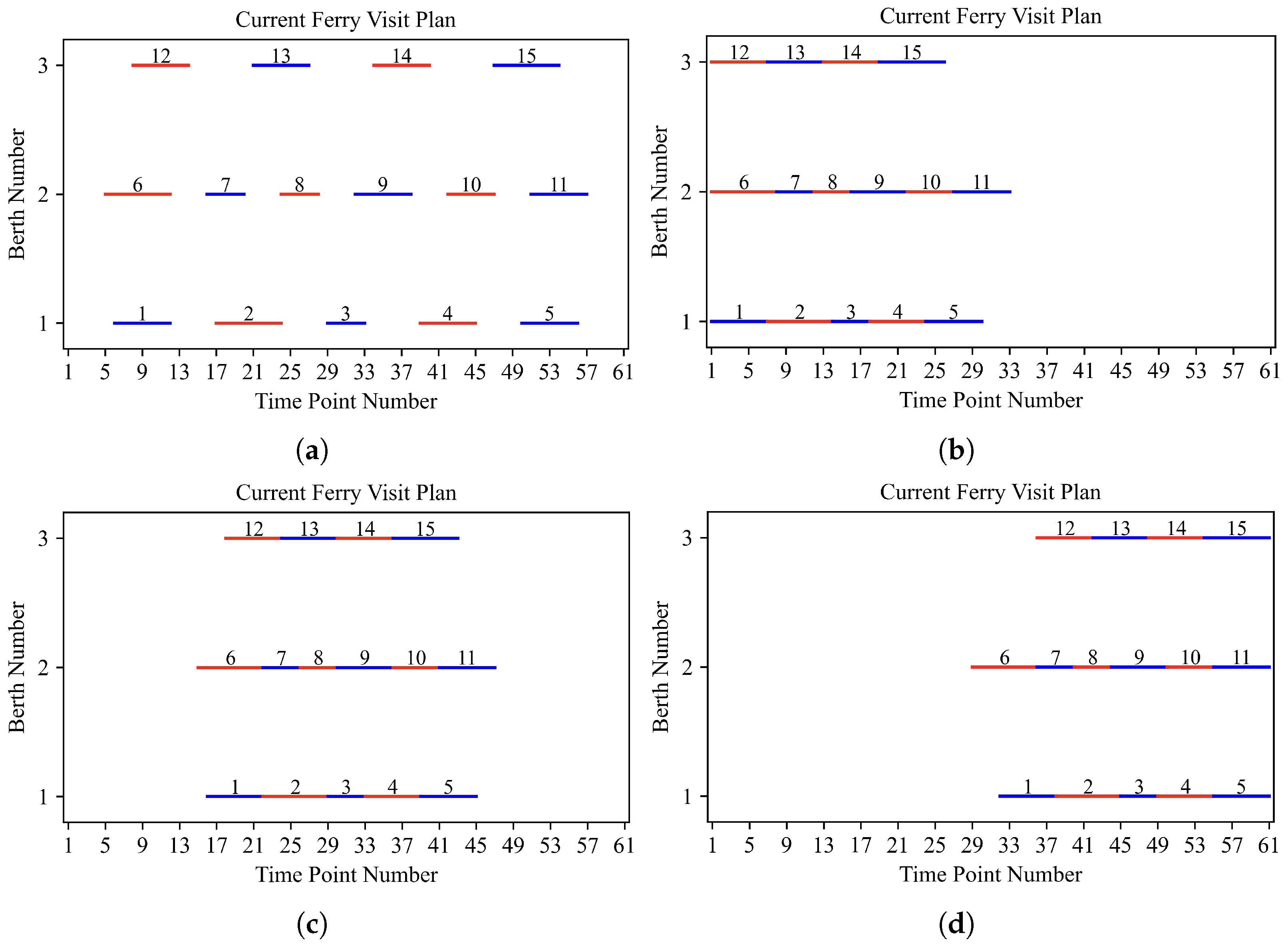
5.2.1. Different Distribution Patterns of Existing Ferry Visits

Numerical experiments with different distribution patterns of the existing ferry visits are conducted in this subsection. In this paper, we consider five different distribution patterns. In detail, distribution pattern 1 is our current ferry visit plan in Figure 2. The remaining four distribution patterns are shown in Figure 5. In distribution pattern 2, shown in Figure 5a, all the 15 existing ferry visits are equally distributed during the operational period. In distribution pattern 3, shown in Figure 5b, all the 15 existing ferry visits are arranged to serve the ferry passengers during the early time periods of the operational period. In distribution pattern 4, shown in Figure 5c, 15 existing ferry visits serve the ferry passengers in the middle time periods of the operational period. In distribution pattern 4, shown in Figure 5d, 15 existing ferry visits serve the ferry passengers at the late time periods of the operational period. Similar to Figure 2, the red and blue in Figure 5a–d are used to distinguish different ferry visits that arrive in adjacent order and moor at the same berth.

Detailed results of our model and the inserting algorithm under different distribution patterns of existing ferry visits are listed in

Table 4. Detailed results of our model under different distribution patterns of existing ferry visits.

Distribution	TP	TR	TPBL	TPBT	TPST	CPU (s)
1	84,336.15	85,519.06	0.00	0.00	−1182.91	374.71
2	89,363.13	92,006.14	−639.50	0.00	−2003.52	7201.69
3	86,259.97	92,497.28	0.00	−3837.00	−2400.31	7201.86
4	91,118.18	94,912.04	0.00	0.00	−3793.86	361.77
5	88,977.05	94,073.01	0.00	−959.25	−4136.71	143.41

and

Table 5. Detailed results of the inserting algorithm under different distribution patterns of existing ferry visits.

Distribution	TP	TR	TPBL	TPBT	TPST	CPU (s)
1	76,136.75	82,224.35	0.00	0.00	−6087.60	0.64
2	82,009.92	88,097.52	0.00	0.00	−6087.60	0.63
3	81,129.97	87,217.57	0.00	0.00	−6087.60	0.65
4	85,754.83	91,842.43	0.00	0.00	−6087.60	0.66
5	84,281.42	90,369.02	0.00	0.00	−6087.60	0.66

. In Table 4 and Table 5, TP, TR, TPBL, TPBT, TPST, and CPU represent the total profit, the total revenue, the total penalty for berthing location deviation, the total penalty for berthing time deviation, the total penalty for servicing time deviation, and computational time. From Table 4 and Table 5, we can find that distribution pattern 4 has the largest total profit (i.e., USD 91,118.18 using our model and USD 85,754.83 using the inserting algorithm). This is mainly because the revenue at the middle time points is generally much higher than that at the early or late time points.

Table 6. The comparison between our model and the inserting algorithm under different distribution patterns of existing ferry visits.

Distribution	TP		D (%)	CPU (s)
	A1	A2		A1	A2
1	84,336.15	76,136.75	9.72	374.71	0.64
2	89,363.13	82,009.92	8.23	7201.69	0.63
3	86,259.97	81,129.97	5.95	7201.86	0.65
4	91,118.18	85,754.83	5.89	361.77	0.66
5	88,977.05	84,281.42	5.28	143.41	0.66

shows the comparison between our model and the inserting algorithm. In Table 6, A1 represents our model and A2 represents the inserting algorithm. D represents the difference of the total profit obtained by our mode and that obtained by the inserting algorithm, which is calculated by (A1 − A2) × 100%/A1. From Table 6, we can find that the total profits obtained by our model are always higher than those obtained by the inserting algorithm. In addition, under distribution patterns 1 and 2, the differences (D(%)) between the total profit obtained by our model and that obtained by the inserting algorithm are much larger. This is mainly because our model is more flexible in adjusting the current visit plan to obtain the optimal solution when the existing ferry visits are scatteredly distributed.

5.2.2. Different Numbers of Existing Ferry Visits and Added Ferry Visits

The numbers of existing visits and added visits are crucial parameters that influence the visit plan optimization. Therefore, a series of instances with different numbers of existing visits and added visits were conducted to show the superiority of the proposed model and solution method. The detailed numbers of existing ferry visits and added ferry visits of each instance are listed as follows.

In Instance 1, there are 10 existing ferry visits and 5 added ferry visits. In Instance 2, the number of the existing ferry visits and added ferry visits are both 10. In Instance 3, the numbers of existing ferry visits and added ferry visits are 10 and 15, respectively. In Instance 4, i.e., basic instance in Section 5.1, there are 15 existing ferry visits and 5 added ferry visits. In Instance 5, the numbers of existing ferry visits and added ferry visits are 15 and 10, respectively. In Instance 6, there are 20 existing ferry visits and 5 added ferry visits. In Instance 7, the numbers of the existing ferry visits and added ferry visits are 20 and 10, respectively. In particular, the occupancy rate of the berth among the seven instances during the operational period ranges from 48.33% to 91.67%.

Detailed results of our model under different numbers of existing and added ferry visits are listed in

Table 7. Detailed results of our model under different numbers of existing and added ferry visits.

Instance	TP	TR	TPBL	TPBT	TPST	CPU (s)
1	64,775.23	67,572.13	0.00	−1918.50	−878.41	649.12
2	85,445.62	86,542.26	0.00	0.00	−1096.64	7202.06
3	103,752.34	105,717.03	0.00	0.00	−1964.68	7201.80
4	84,336.15	85,519.06	0.00	0.00	−1182.91	374.71
5	102,497.43	106,023.99	0.00	0.00	−3526.56	7201.53
6	101,366.75	104,243.62	0.00	0.00	−2876.86	665.04
7	111,475.01	124,359.73	−1918.50	−2877.75	−8088.47	7201.64

, in which TP represents the total profit, TR denotes the total revenue, TPBL means the total penalty for berthing location deviation, TPBT represents the total penalty for berthing time deviation, and TPST denotes the total penalty for servicing time deviation. From Table 7, we can find that the total profit obtained by Instance 7 is the largest (USD 111,475.01) among these seven instances. This is mainly because Instance 7 has the maximum number of ferry visits, with a total of 30 ferry visits. In addition, we can find that the instance with more ferry visits generally has higher total profits. For example, the total profit of Instance 3 (i.e., 25 ferry visits) is higher than that of Instance 1 (i.e., 15 ferry visits).

Detailed results of the inserting algorithm under different numbers of existing and added ferry visits are listed in

Table 8. Detailed results of the inserting algorithm under different numbers of existing and added ferry visits.

Instance	TP	TR	TPBL	TPBT	TPST	CPU (s)
1	59,179.66	63,745.36	0.00	0.00	−4565.70	0.71
2	75,788.86	81,876.46	0.00	0.00	−6087.60	0.73
3	96,531.79	104,141.30	0.00	0.00	−7609.50	0.75
4	76,136.75	82,224.35	0.00	0.00	−6087.60	0.64
5	96,409.01	104,018.51	0.00	0.00	−7609.50	0.65
6	96,409.01	104,018.51	0.00	0.00	−7609.50	0.71
7	-	-	-	-	-	-

. In Table 8, the total profit of Instance 3 is the largest: USD 96,531.79. In addition, the instance with more ferry visits has higher total profits. Note that the inserting algorithm cannot find the optimal solution for Instance 7 within 7200 s.

The comparison between our model and the inserting algorithm under different numbers of existing and added ferry visits is shown in

Table 9. The comparison between our model and the inserting algorithm under different numbers of existing and added ferry visits.

Instance	TP		D (%)	CPU (s)
	A1	A2		A1	A2
1	64,775.23	59,179.66	8.64	649.12	0.71
2	85,445.62	75,788.86	11.30	7202.06	0.73
3	103,752.34	96,531.79	6.96	7201.80	0.75
4	84,336.15	76,136.75	9.72	374.71	0.64
5	102,497.43	96,409.01	5.94	7201.53	0.65
6	101,366.75	96,409.01	4.89	665.04	0.71
7	111,475.01	-	-	7201.64	-

. From the Table 9, it is obvious that the total profit obtained by our model is always higher than that obtained by the inserting algorithm among all the seven instances. This demonstrates that the performance of our model is superior to that of the inserting algorithm. Note that for Instance 2, the difference between our model and the inserting algorithm is as high as 11.3%.

5.2.3. Range of Expectation of the Real Time Taken by All the Ferry Visits

The expectation of the real servicing time reveals the number of ferry passengers. When the passenger demand is higher, the servicing time for boarding and disembarking passengers is generally longer. In our study, the expectations of servicing time also impact the difficulty in arranging the visit plan. Thus, in this subsection, we conduct numerical experiments with different expectation ranges of servicing time, namely, 20 to 50 min (i.e., maximum value, 50 min; minimum value, 20 min), 30 to 60 min (the basic instance) (i.e., maximum value, 60 min; minimum value, 30 min), and 40 to 70 min (i.e., maximum value, 70 min; minimum value, 40 min), to show the influence of the number of ferry passengers on the total profit.

In comparison to Instance 1, the expectation of real servicing time ranges from 20 min to 50 min. Since the real servicing time becomes shorter than the basic instance, we then adjust the revenue at the different time points. Specifically, we first reduce the number of ferry passengers by 10% except for time point 31. Time point 31 still has the highest ferry passenger demand, in accordance with the setting in Section 5.1. The revenue at different time points changes. Comparison Instance 2 is the basic instance in Section 5.1. Hence, the revenue at different time points keeps unchanged. In Comparison Instance 3, the expectation of real servicing time ranges from 40 min to 70 min. Similar to Comparison Instance 1, we also adjust the number of passengers. In detail, the number of passengers at different time points increases by 10%. However, due to the capacity constraint of the ferry ship, the number of passengers at time point 31 is also 243. Meanwhile, if the number of passengers at some time points (excluding time point $t=31$) exceeds 243, the number of passengers will be equal to 243 minus a random number between 1 and 4. Then, the revenue at different time points changes.

Detailed results of our model and the inserting algorithm under different ranges of expectation of the real servicing time of all ferry visits are listed in

Table 10. Detailed results of our model under different ranges of expectation of the real time of all ferry visits.

Expectation	TP	TR	TPBL	TPBT	TPST	CPU (s)
(20,50)	77,669.89	80,157.49	0.00	959.25	1528.34	47.16
(30,60)	84,336.15	85,519.06	0.00	0.00	−1182.91	374.71
(40,70)	88,562.05	90,962.48	0.00	0.00	−2400.43	7201.65

and

Table 11. Detailed results of the inserting algorithm under different ranges of expectation of the real time of all ferry visits.

Expectation	TP	TR	TPBL	TPBT	TPST	CPU (s)
(20,50)	69,138.06	75,225.66	0.00	0.00	6087.60	0.72
(30,60)	76,136.75	82,224.35	0.00	0.00	−6087.60	0.64
(40,70)	83,074.05	83,074.05	0.00	0.00	−6087.60	0.73

, respectively. “TP”, “TR”, “TPBL”, “TPBT”, and “TPST” in Table 10 and Table 11 represent the same meanings as those in Table 7. In Table 10, when the expectation of the real servicing time increases, the total profit (TP) and the total revenue (TR) increase, which is mainly due to the increased revenue at different time points. In addition, the computation time (CPU (s)) increases with the increase in expectations of real servicing time. In Table 11, the total profit and total revenue also increase with the expectations of real servicing time, which is similar to the results obtained by our model. In addition, the comparison between our model and the inserting algorithm is shown in

Table 12. The comparison between our model and the inserting algorithm under different ranges of expectation of the real time of all ferry visits.

Expectation	TP		D (%)	CPU (s)
	A1	A2		A1	A2
(20,50)	77,669.89	69,138.06	9.72	47.16	0.72
(30,60)	84,336.15	76,136.75	9.72	374.71	0.64
(40,70)	88,562.05	83,074.05	6.20	7201.65	0.73

. “A1”, “A2”, and “D” have the same meanings as those in Table 9. From Table 12, it is obvious that our model shows a better performance in obtaining the total profit than the inserting algorithm. In addition, the difference (D) between our model and the inserting algorithm becomes smaller when the expectation of the real servicing time increases. This may be because the number of feasible solutions decreases.

6. Conclusions

In this study, we investigated the ferry visit planning problem, considering adding new visits on the basis of the current ferry visit plan. Compared to the existing research related to ferry transportation, this is the first paper that considers the three practical aspects of ferry visits during the operational period, which are uncertain servicing time, time-dependent revenue, and deviation between the redesigned ferry visit plan and the current one, respectively. By considering these practical aspects, our model can help the ferry company devise a more scientific and reasonable ferry visit plan to obtain the maximum profit. To model our investigated problem, a mixed-integer nonlinear programming model with stochastic servicing time of each visit is formulated. By adding new variables and constraints, the stochastic servicing time was converted into constraints on the minimum berthing time slots allocated to each visit and the penalty of the real servicing exceeding the allocated time in the objective function. Other nonlinear elements were handled in the traditional way.

Numerical experiments based on real data collected from the official website of the Hong Kong Macau Ferry Terminal in Hong Kong were conducted to validate the proposed model and solution method. After adding five ferry visits (redesigned ferry visit plan with 20 ferry visits), a total profit of USD 84,336.14 is obtained, which is larger than the total profit obtained by performing the current ferry visit plan with 15 ferry visits (i.e., USD 62,374.27). Then, an inserting algorithm was also developed to solve the problem and represent the manual decision process. Compared to our model, the inserting algorithm only realized a total profit of USD 76,136.74, which is much lower than the profit obtained by our model. Sensitive analyses on visit number, expectation of the servicing time, and visits distribution pattern validate the superiority of the model and solution method originally proposed. There were several findings: (1) Under different numbers of existing ferry visits and added ferry visits, our model and solution method can further improve the total profit compared to the inserting algorithm. (2) When the expectation of real servicing time becomes larger, the difference between the optimal objective values of our model and the inserting algorithm decreases. (3) When the existing ferry visits are scattered, our model has an obvious advantage in obtaining higher profits compared to the inserting algorithm.

This study has its own limitations. First, in this paper, identical ports and ferry ships were considered. However, ships and berths with various capacities are deployed and provided in practice. Second, the deployment details of ferry ships were not taken into account in this study. For short ferry routes, the deployment of ships will also influence the berth allocation plan. Third, we only consider one ferry terminal in this paper. Based on these limitations, there are elements that could be integrated into future research: heterogeneous ships and berths, deployment of ferry vessels, and multiple terminals in the same ferry shipping network.

References

1. Lau, Y.; Tam, K.; Ng, A.K. Ferry services and the community development of peripheral island areas in Hong Kong: Evidence from Cheung Chau. Isl. Stud. J. 2023, 1–25. [Google Scholar] [CrossRef]
2. Transportnsw.Info. Ferry|Transportnsw.Info. 2023. Available online: https://transportnsw.info/travel-info/ways-to-get-around/ferry#/ (accessed on 4 May 2023).
3. Lai, M.; Lo, H.K. Ferry service network design: Optimal fleet size, routing, and scheduling. Transp. Res. Part A Policy Pract. 2004, 38, 305–328. [Google Scholar] [CrossRef]
4. Wang, D.Z.; Lo, H.K. Multi-fleet ferry service network design with passenger preferences for differential services. Transp. Res. Part B Methodol. 2008, 42, 798–822. [Google Scholar] [CrossRef]
5. Lo, H.K.; An, K.; Lin, W.H. Ferry service network design under demand uncertainty. Transp. Res. Part E Logist. Transp. Rev. 2013, 59, 48–70. [Google Scholar] [CrossRef]
6. An, K.; Lo, H.K. Ferry service network design with stochastic demand under user equilibrium flows. Transp. Res. Part B Methodol. 2014, 66, 70–89. [Google Scholar] [CrossRef]
7. Ng, M.; Lo, H.K. Robust models for transportation service network design. Transp. Res. Part B Methodol. 2016, 94, 378–386. [Google Scholar] [CrossRef]
8. Bell, M.G.; Pan, J.J.; Teye, C.; Cheung, K.F.; Perera, S. An entropy maximizing approach to the ferry network design problem. Transp. Res. Part B Methodol. 2020, 132, 15–28. [Google Scholar] [CrossRef]
9. Aslaksen, I.E.; Svanberg, E.; Fagerholt, K.; Johnsen, L.C.; Meisel, F. Ferry service network design for kiel fjord. In Proceedings of the Computational Logistics: 11th International Conference, ICCL 2020, Enschede, The Netherlands, 28–30 September 2020; Springer: Berlin/Heidelberg, Germany, 2020; pp. 36–51. [Google Scholar]
10. Aslaksen, I.E.; Svanberg, E.; Fagerholt, K.; Johnsen, L.C.; Meisel, F. A combined dial-a-ride and fixed schedule ferry service for coastal cities. Transp. Res. Part A Policy Pract. 2021, 153, 306–325. [Google Scholar]
11. Imai, A.; Nagaiwa, K.; Tat, C.W. Efficient planning of berth allocation for container terminals in Asia. J. Adv. Transp. 1997, 31, 75–94. [Google Scholar] [CrossRef]
12. Liu, C. Iterative heuristic for simultaneous allocations of berths, quay cranes, and yards under practical situations. Transp. Res. Part E Logist. Transp. Rev. 2020, 133, 101814. [Google Scholar] [CrossRef]
13. Chargui, K.; Zouadi, T.; El Fallahi, A.; Reghioui, M.; Aouam, T. Berth and quay crane allocation and scheduling with worker performance variability and yard truck deployment in container terminals. Transp. Res. Part E Logist. Transp. Rev. 2021, 154, 102449. [Google Scholar] [CrossRef]
14. Rodrigues, F.; Agra, A. Berth allocation and quay crane assignment/scheduling problem under uncertainty: A survey. Eur. J. Oper. Res. 2022, 303, 501–524. [Google Scholar]
15. Han, X.L.; Lu, Z.Q.; Xi, L.F. A proactive approach for simultaneous berth and quay crane scheduling problem with stochastic arrival and handling time. Eur. J. Oper. Res. 2010, 207, 1327–1340. [Google Scholar] [CrossRef]
16. Zhen, L.; Lee, L.H.; Chew, E.P. A decision model for berth allocation under uncertainty. Eur. J. Oper. Res. 2011, 212, 54–68. [Google Scholar]
17. Umang, N.; Bierlaire, M.; Vacca, I. Exact and heuristic methods to solve the berth allocation problem in bulk ports. Transp. Res. Part E Logist. Transp. Rev. 2013, 54, 14–31. [Google Scholar] [CrossRef]
18. Ursavas, E.; Zhu, S.X. Optimal policies for the berth allocation problem under stochastic nature. Eur. J. Oper. Res. 2016, 255, 380–387. [Google Scholar]
19. Zhen, L.; Chang, D.F. A bi-objective model for robust berth allocation scheduling. Comput. Ind. Eng. 2012, 63, 262–273. [Google Scholar] [CrossRef]
20. Shang, X.T.; Cao, J.X.; Ren, J. A robust optimization approach to the integrated berth allocation and quay crane assignment problem. Transp. Res. Part E Logist. Transp. Rev. 2016, 94, 44–65. [Google Scholar]
21. Xiang, X.; Liu, C.; Miao, L. A bi-objective robust model for berth allocation scheduling under uncertainty. Transp. Res. Part E Logist. Transp. Rev. 2017, 106, 294–319. [Google Scholar]
22. Iris, Ç.; Lam, J.S.L. Recoverable robustness in weekly berth and quay crane planning. Transp. Res. Part B Methodol. 2019, 122, 365–389. [Google Scholar]
23. Li, M.Z.; Jin, J.G.; Lu, C.X. Real-time disruption recovery for integrated berth allocation and crane assignment in container terminals. Transp. Res. Rec. 2015, 2479, 49–59. [Google Scholar] [CrossRef]
24. Liu, C.; Zheng, L.; Zhang, C. Behavior perception-based disruption models for berth allocation and quay crane assignment problems. Comput. Ind. Eng. 2016, 97, 258–275. [Google Scholar]
25. Nourmohammadzadeh, A.; Voss, S. A robust multiobjective model for the integrated berth and quay crane scheduling problem at seaside container terminals. Ann. Math. Artif. Intell. 2022, 90, 831–853. [Google Scholar]
26. Xiang, X.; Liu, C.; Miao, L. Reactive strategy for discrete berth allocation and quay crane assignment problems under uncertainty. Comput. Ind. Eng. 2018, 126, 196–216. [Google Scholar]
27. Al-Refaie, A.; Abedalqader, H. Optimal berth scheduling and sequencing under unexpected events. J. Oper. Res. Soc. 2020, 73, 430–444. [Google Scholar] [CrossRef]
28. Park, H.J.; Cho, S.W.; Lee, C. Particle swarm optimization algorithm with time buffer insertion for robust berth scheduling. Comput. Ind. Eng. 2021, 160, 107585. [Google Scholar]
29. Rodrigues, F.; Agra, A. An exact robust approach for the integrated berth allocation and quay crane scheduling problem under uncertain arrival times. Eur. J. Oper. Res. 2021, 295, 499–516. [Google Scholar] [CrossRef]
30. Guo, L.; Zheng, J.; Du, H.; Du, J.; Zhu, Z. The berth assignment and allocation problem considering cooperative liner carriers. Transp. Res. Part E Logist. Transp. Rev. 2022, 164, 102793. [Google Scholar]
31. Xiang, X.; Liu, C. An expanded robust optimisation approach for the berth allocation problem considering uncertain operation time. Omega 2021, 103, 102444. [Google Scholar]
32. Agra, A.; Rodrigues, F. Distributionally robust optimization for the berth allocation problem under uncertainty. Transp. Res. Part B Methodol. 2022, 164, 1–24. [Google Scholar]
33. Zhen, L.; Zhuge, D.; Wang, S.; Wang, K. Integrated berth and yard space allocation under uncertainty. Transp. Res. Part B Methodol. 2022, 162, 1–27. [Google Scholar] [CrossRef]
34. Liu, B.; Li, Z.C.; Wang, Y. A two-stage stochastic programming model for seaport berth and channel planning with uncertainties in ship arrival and handling times. Transp. Res. Part E Logist. Transp. Rev. 2022, 167, 102919. [Google Scholar] [CrossRef]
35. TurboJET. Shipping Schedule/Price List of TurboJET. 2023. Available online: https://www.turbojet.com.hk/tc/routing-sailing-schedule/hong-kong-macau/sailing-schedule-fares.aspx (accessed on 10 May 2023).
36. TurboJET. Ferry Fleet Information of TurboJET. 2023. Available online: https://www.turbojet.com.hk/tc/vessel-information/vessel-summary.aspx (accessed on 28 April 2023).
Figure 1. An illustration of actual and allocated servicing time.
Jmse 11 01644 g001
Figure 2. Berth utilization of the current plan.
Jmse 11 01644 g002
Figure 3. Berth utilization of the redesigned ferry visit plan.
Jmse 11 01644 g003
Figure 4. Berth utilization of visit plan in the generated instance.
Jmse 11 01644 g004
Figure 5. Different distribution patterns of existing ferry visits. (a) Distribution pattern 2. (b) Distribution pattern 3. (c) Distribution pattern 4. (d) Distribution pattern 5.
Jmse 11 01644 g005