Distributed Event-Triggered Fixed-Time Leader–Follower Formation Tracking Control of Multiple Underwater Vehicles Based on an Adaptive Fixed-Time Observer

Abstract

This paper focuses on the fixed-time leader–follower formation control of multiple underwater vehicles (MUVs) in the presence of external disturbances. First, an adaptive fixed-time disturbance observer (AFxDO) is developed to deal with unknown time-varying environmental disturbances. The developed AFxDO guarantees the fixed-time convergence property of the disturbance observation error and no prior information on the external disturbances or their derivatives is required. Then, with the aid of the developed AFxDO, a distributed event-triggered fixed-time backstepping controller was developed to achieve the leader–follower formation tracking control of MUVs. To solve the “explosion of complexity” problem inherent in the conventional backstepping, a nonlinear filter is introduced to obtain the derivative of the virtual control law. Furthermore, to reduce the communication burden, the event-triggered mechanism is integrated into the formation tracking controller. The stability analysis shows that the closed-loop MUV system is practical fixed-time stable. Finally, simulation results demonstrate the effectiveness of the proposed scheme.

1. Introduction

Nowadays, multi-agent systems have garnered widespread attention due to their emerging applications in many fields [1,2]. As a typical multi-agent system, underwater vehicles have become important tools for ocean exploitation and are extensively used in oceanographic observations, hydrology research, target tracking, and so on [3,4,5,6]. To broaden the service coverage and enhance the system reliability, the cooperative control of multiple underwater vehicles (MUVs) has been increasingly deployed to perform complex and large missions. However, the control of MUVs is a challenging problem because of the effect of adverse factors such as strong nonlinearity and unknown time-varying external disturbances [7,8]. Various methods have been presented to achieve cooperative control of MUVs [9,10,11]. Among the existing cooperative control methods, the leader–follower formation control approach has been diffusely applied due to its reliability [12].

For leader–follower formation control of MUVs, coordination convergence is a critical performance index and has become a research hotspot. In [13], a distributed event-triggered control law was proposed for the formation tracking of MUVs, where an adaptive neural network observer was developed to estimate the local velocity information. In [14], a distributed Lyapunov-based model predictive control (MPC) law was presented for a team of underwater vehicles, where an extended state observer (ESO) was developed for handling environmental disturbances. However, the above control laws can only achieve the asymptotic stability of the formation control system, meaning that the settling time tends to infinity [15,16]. The finite-time control is extensively studied on account of its better performance on convergence rate and robustness than the asymptotic control. In [17], the finite-time consensus tracking of MUVs was investigated and an adaptive sliding mode control (SMC) method was presented to guarantee the finite-time stability. Unfortunately, the upper bound of the convergence time of the finite-time control is related to the initial conditions of the system [18,19,20]. Since the initial conditions are difficult to obtain in practical engineering scenarios, finite control is limited in its applications [21,22,23]. To handle these constraints, the fixed-time control is presented to ensure that the convergence time is upper-bounded by an a priori value, irrespective of the initial conditions, and only control parameters are associated [24]. In [25], a fixed-time sliding mode formation controller was proposed. In [26], a fast fixed-time SMC law was presented. However, the above control laws only consider horizontal plane formation control.

To handle the formation control of MUVs subject to external disturbances, different approaches have been proposed, such as adaptive parameter estimation and disturbance observers [27]. In [28], an adaptive finite-time formation control law was developed for MUVs with external disturbances. However, the reconstruction information about the external disturbances could not be obtained. The disturbance observer is an effective way to reconstruct external disturbances and it is becoming increasingly popular. In [29], a disturbance estimator was presented to deal with the unknown dynamic and disturbances. In [30], a finite-time ESO was proposed to estimate the system uncertainties. However, their observation errors can only achieve asymptotic or finite-time convergence. In [25,31], a fixed-time disturbance observer was developed, where the fixed-time convergence of the disturbance observation errors was guaranteed. Nevertheless, the upper bounds or the derivative upper bounds of the disturbances were assumed to be known in advance, which is a strict limitation for practical applications. To solve these problems, this paper presents an adaptive fixed-time disturbance observer (AFxDO). With the developed AFxDO, the rigorous restriction on prior information of disturbances is removed by designing the adaptive parameter estimation strategy, and the fixed-time stability of the observation errors is guaranteed at the same time.

Given the actual working conditions, the communication devices of underwater vehicles often face constraints [32]. Saving communication bandwidth and computing resources should be taken into consideration when designing the formation controller of MUVs [33]. In the literature, the event-triggered control has been studied by many researchers in formation control due to the efficient management of control signals [34]. In [35], the consensus problem of MUVs was studied, where an adaptive dynamic event-triggered mechanism was presented to reduce the transmission burden. In [36], a distributed adaptive event-triggered formation control law was developed for MUVs. Although the control schemes mentioned above adopt the event-triggering mechanism, most of them cannot guarantee the fixed-time stability of tracking errors.

Motivated by the aforementioned analyses, in this paper, an AFxDO-based distributed event-triggered fixed-time leader–follower formation trajectory tracking control methodology was developed for MUVs subject to unknown time-varying external disturbances under a directed network. The main contributions of this paper are as follows:

• A novel AFxDO combined with an adaptive parameter estimation strategy was developed to eliminate the adverse effects of unknown time-varying external disturbances. Unlike existing disturbance observers, the proposed AFxDO guarantees the fixed-time stability of the observation errors, and the strict limitation of the prior information of the bound value of external disturbances was removed through the adaptive parameter estimation strategy.
• Together with the developed AFxDO, a distributed event-triggered fixed-time backstepping control strategy is proposed to solve the leader–follower formation control problem for MUVs subject to external disturbances. A nonlinear first-order filter was designed to avoid the “explosion of complexity” problem in conventional backstepping approach. The proposed formation tracking control methodology ensures that the formation tracking errors converge to an arbitrarily small neighborhood around the origin within a fixed time, independent of initial conditions. Additionally, the bandwidth resources are saved and the communication burdens are reduced by introducing an event-triggered mechanism.

This paper is organized as follows. The model description and preliminaries are described in Section 2. The main results are given in Section 3, where the design and stability analysis of the AFxDO and the distributed event-triggered fixed-time backstepping controller are presented. The simulation results are provided in Section 4. The paper ends with concluding remarks in Section 5.

2. Model Description and Preliminaries

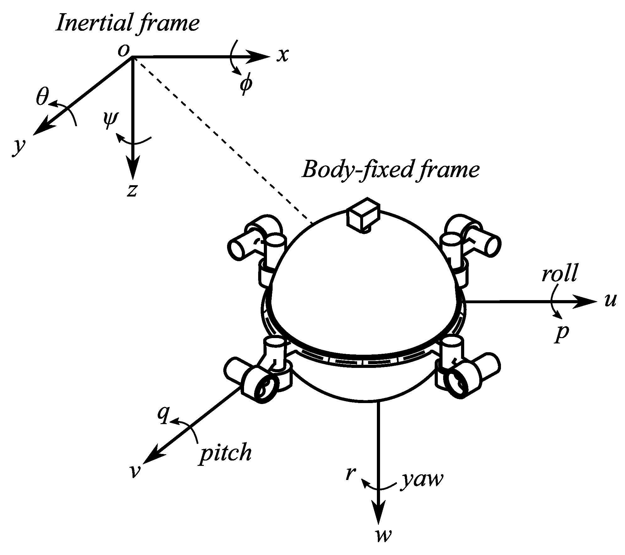
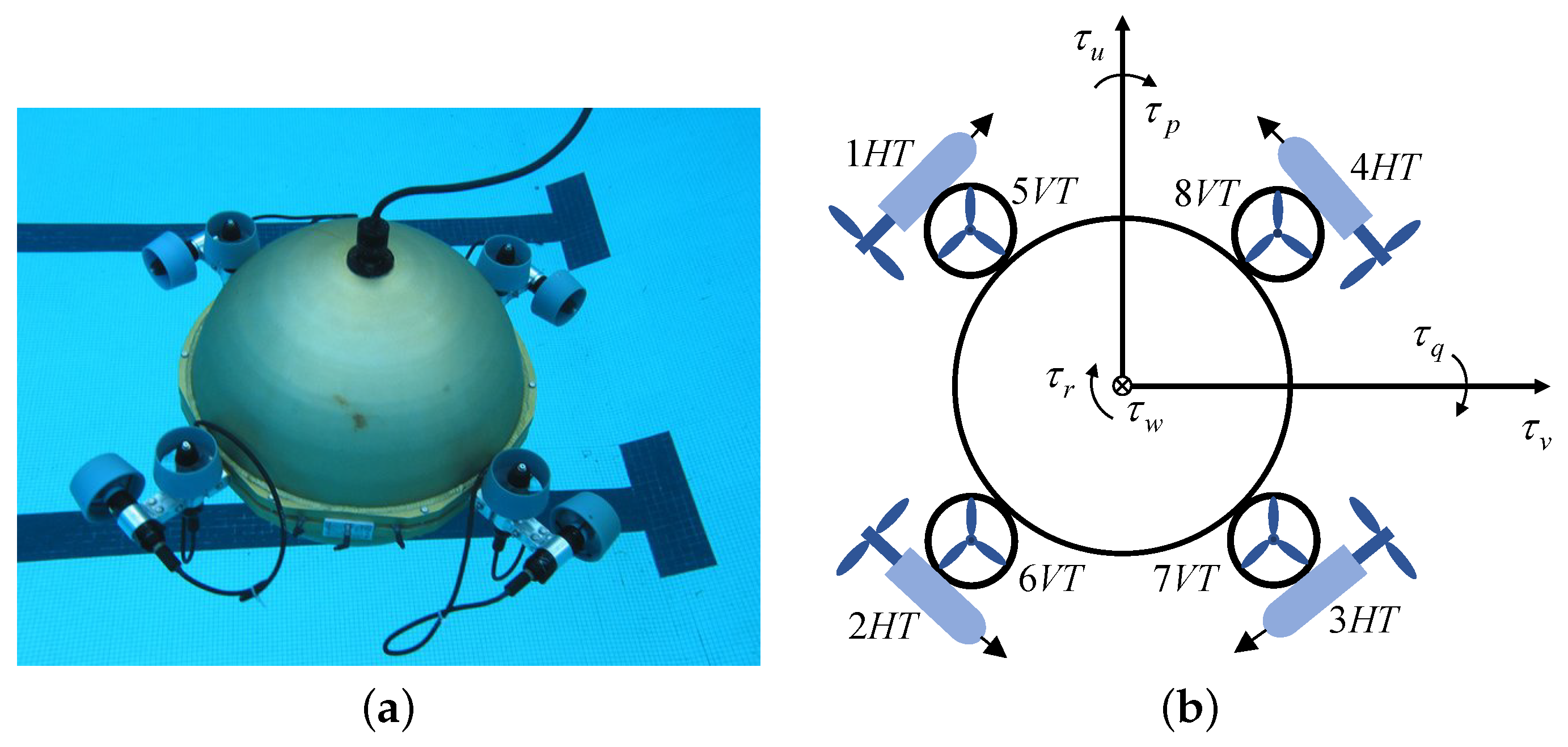
2.1. Modeling of Networked Underwater Vehicles

Consider a group of homogeneous underwater vehicles composed of followers (labeled as $1,\cdots ,n$) and a leader (labeled as 0) under a directed communication topology. In order to establish the six degrees of freedom (DOF) motion model of each underwater vehicle, we introduce two reference frames, namely, the inertial frame and body-fixed frame. As shown in Figure 1, the inertial frame is located on Earth, and the body-fixed frame is located in the center of mass of the vehicle. In the inertial frame, the position and attitude vector of the underwater vehicle is defined as $\mathit{\eta }={\left[x,y,z,\varphi ,\theta ,\psi \right]}^T$, while in the body-fixed frame, the linear and angular velocity vectors are defined as $\mathit{\nu }={\left[u,v,w,p,q,r\right]}^T$. Based on the defined frames and coordinate vectors, the 6 DOF kinematics and dynamics equations of the ith underwater vehicle can be described as [37]:

$$\begin{array}{c}\hfill \left\{\begin{array}{c}{\dot{\mathit{\eta }}}_i={\mathit{J}}_i\left({\mathit{\eta }}_i\right){\mathit{\nu }}_i\hfill \\ {\mathit{M}}_i{\dot{\mathit{\nu }}}_i+{\mathit{C}}_i\left({\mathit{\nu }}_i\right){\mathit{\nu }}_i+{\mathit{D}}_i\left({\mathit{\nu }}_i\right){\mathit{\nu }}_i+{\mathit{g}}_i\left({\mathit{\eta }}_i\right)={\mathit{\tau }}_i+{\mathit{f}}_i\hfill \end{array}\right.,\end{array}$$

(1)

where ${\mathit{J}}_i\left({\mathit{\eta }}_i\right)$ is the Jacobian transformation matrix describing the relationship between the inertial frame and body-fixed frame; ${\mathit{M}}_i\in {\mathbb{R}}^{6\times 6}$ is the inertia matrix of underwater vehicles, including the rigidity mass and the additional mass; ${\mathit{C}}_i\left({\mathit{\nu }}_i\right)\in {\mathbb{R}}^{6\times 6}$ is the Coriolis and centrifugal matrix; ${\mathit{D}}_i\left({\mathit{\nu }}_i\right)\in {\mathbb{R}}^{6\times 6}$ is the hydrodynamic damping matrix; ${\mathit{g}}_i\left({\mathit{\eta }}_i\right)\in {\mathbb{R}}^6$ is the restoring forces (gravity and buoyancy) vector; ${\mathit{f}}_i\in {\mathbb{R}}^6$ is the unknown time-varying external disturbances vector caused by ocean currents and waves; ${\mathit{\tau }}_i\in {\mathbb{R}}^6$ is the vector of control forces and moments of propellants.

Assumption A1. 

The Jacobian transformation matrix ${\mathit{J}}_i\left({\mathit{\eta }}_i\right)$ is bounded, i.e., there exists known positive constants ${\overline{J}}_i$ such that $\parallel {\mathit{J}}_i\left({\mathit{\eta }}_i\right)\parallel \le {\overline{J}}_i$.

Assumption A2. 

The external disturbances ${\mathit{f}}_i$ are supposed to be unknown but bounded, such that $\parallel {\mathit{f}}_i\parallel \le \gamma$, where γ is the unknown upper bound of external disturbances.

2.2. Notation and Related Lemmas

In this paper, ${\mathit{x}}^T$ denotes the transpose of vector $\mathit{x}$, $\parallel \mathit{x}\parallel$ denotes the Euclidean norm of vector $\mathit{x}$, ${\sigma }_{min}(·)/{\sigma }_{max}(·)$ denotes the minimum/maximum eigenvalue of a matrix, ${\mathit{sig}}^a\left(\mathit{x}\right)={\left[|x_1{|}^a\mathrm{sign}\left(x_1\right),|x_2{|}^a\mathrm{sign}\left(x_2\right),\dots ,{\left|x_n\right|}^a\mathrm{sign}\left(x_n\right)\right]}^T$ where sign(·) is the sign function, and $tanh\left(\mathit{x}\right)={[tanh\left(x_1\right),tanh\left(x_2\right),\dots ,tanh\left(x_n\right)]}^T$.

Consider a nonlinear system

$$\begin{array}{c}\hfill \dot{\mathit{x}}\left(t\right)=\mathit{f}\left(\mathit{x}\left(t\right)\right),f\left(0\right)=0,\end{array}$$

(2)

where $\mathit{x}={[x_1,x_2,\dots ,x_n]}^T\in {\mathbb{R}}^n$ and $\mathit{f}\left(\mathit{x}\right):{\mathbb{R}}^n⟶{\mathbb{R}}^n$ is a nonlinear function.

Definition 1 

([25,39]). The equilibrium $x=0$ of system (2) is fixed-time stable if it is globally finite-time stable and the settling time function $T\left(x\right)$ is bounded by a positive constant $T_{max}$, i.e., $T\left(x\right)\le T_{max}$ for any $x\in {\mathbb{R}}^n$.

Lemma 1 

([25]). For positive constants $a,b,\alpha ,\beta$ with $0<\alpha <1,\beta >1$, if we define a Lyapunov candidate function $V\left(x\right)$ on a neighborhood $U\subset {\mathbb{R}}^n$, satisfying

$$\begin{array}{c}\hfill \dot{V}\left(x\right)\le -a{V}^{\alpha }\left(x\right)-b{V}^{\beta }\left(x\right),\end{array}$$

(3)

then the origin of (2) is fixed-time stable and the settling time T satisfies

$$\begin{array}{c}\hfill T\le T_{max}=\frac{1}{a}\frac{1}{1-\alpha }+\frac{1}{b}\frac{1}{\beta -1}.\end{array}$$

(4)

Remark 1. 

As reported in [24,25,26], the settling time of the finite-time stable system depends on the initial condition. Unlike the finite-time stable system, the convergence time of the fixed-time stable system in Lemma 1 is bounded by an a priori value, which is not determined by the initial condition but by the control parameters $a,b,\alpha ,\beta$. It implies that the settling time can be designed in advance even though the initial condition is unknown.

Lemma 2 

([25]). Suppose the Lyapunov function $V\left(x\right)$ in Lemma 1 satisfies

$$\begin{array}{c}\hfill \dot{V}\left(x\right)\le -a{V}^{\alpha }\left(x\right)-b{V}^{\beta }\left(x\right)+\Omega ,\end{array}$$

(5)

where $\Omega >0$, then the origin of (2) is practical fixed-time stable, and the residual set is given by

$$\begin{array}{c}\hfill \left\{\underset{t\to T_{max}}{lim}x|V\left(x\right)\le min\left\{{\left(\frac{\Omega }{a(1-\omega )}\right)}^{\frac{1}{\alpha }},{\left(\frac{\Omega }{b(1-\omega )}\right)}^{\frac{1}{\beta }}\right\}\right\},\end{array}$$

(6)

where $\omega \in (0,1]$, and T is bounded by

$$\begin{array}{c}\hfill T\le T_{max}=\frac{1}{a\omega (1-\alpha )}+\frac{1}{b\omega (\beta -1)}.\end{array}$$

(7)

Lemma 3 

([40]). For $\forall y\ge x\ge 0$ and $n>1$, we have

$$\begin{array}{c}\hfill x{(y-x)}^n\le \frac{n}{n+1}(y^{n+1}-x^{n+1}).\end{array}$$

(8)

Lemma 4 

([41]). For variables $x\in \mathbb{R},y\in \mathbb{R}$ and constants $a>0,b>0,c>0$, we have

$$\begin{array}{c}\hfill {\left|x\right|}^a{\left|y\right|}^b\le \frac{a}{a+b}{c\left|x\right|}^{a+b}+\frac{b}{a+b}{c}^{-\frac{a}{b}}{\left|y\right|}^{a+b}.\end{array}$$

(9)

Lemma 5 

([34]). For any variable x, the following inequalities hold:

$$\begin{array}{c}\hfill \left|x\right|-xtanh\left(\frac{x}{\varrho }\right)\le \iota \varrho ,\end{array}$$

(10)

where $\varrho >0$ is a constant and $\iota =\underset{t>0}{sup}\left(\frac{1}{1+e^t}\right)=0.2785$.

Lemma 6 

([39]). The following inequalities hold for any nonnegative real number $x_i$,

$$\begin{array}{c}\hfill {\left(\sum _{i=1}^n{x}_i\right)}^a\le \sum _{i=1}^n{x}_i^a,0<a<1,\end{array}$$

(11)

$$\begin{array}{c}\hfill {\left(\sum _{i=1}^n{x}_i\right)}^b\le n^{b-1}\sum _{i=1}^n{x}_i^b,b>1.\end{array}$$

(12)

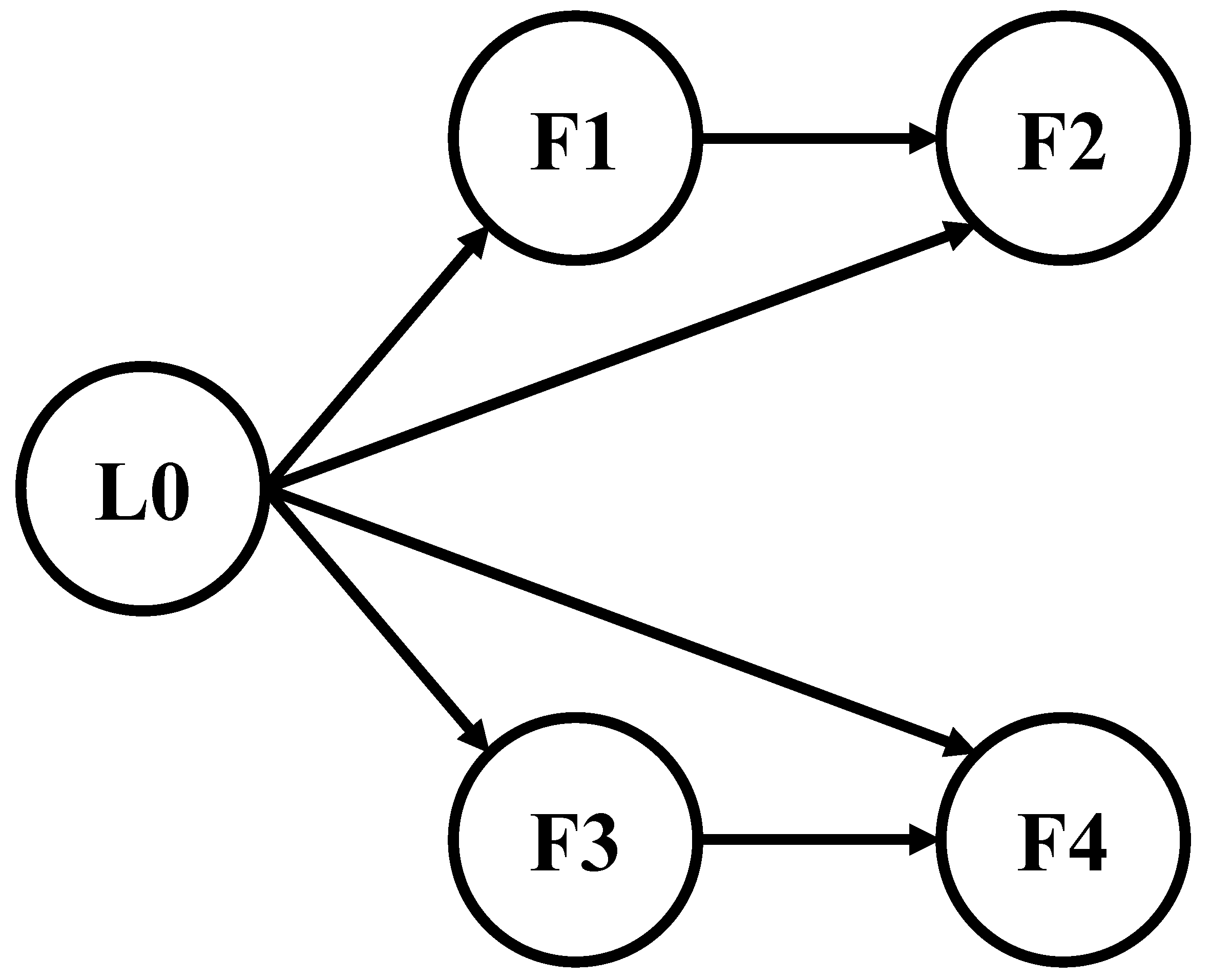
2.3. Basic Graph Theory

The communication topology of the n underwater vehicle followers and a leader is described by a directed graph $\mathit{G}\triangleq \left\{\mathit{N},\mathit{\zeta },\mathit{A}\right\}$, where $N=\{0,1,2,\cdots ,n\}$ and $\mathit{\zeta }\subseteq \mathit{N}\times \mathit{N}$ are the sets of nodes and edges, respectively, and $\mathit{A}=\left[a_{ij}\right]\in {\mathbb{R}}^{n\times n}$ is the adjacency matrix. The information transfer from node $j\in \mathit{N}$ to node $i\in \mathit{N}$ is expressed as $\left({\zeta }_j,{\zeta }_i\right)\in \mathit{\zeta }$, $a_{ij}=1$, node j can be called the neighbor of node i, otherwise, $\left({\zeta }_j,{\zeta }_i\right)\notin \mathit{\zeta }$, $a_{ij}=0$. The in-degree $h_i$ of node i is defined as $h_i={\sum }_{j=0}^n{a}_{ij}$, and the in-degree matrix is defined as $\mathit{H}=\mathrm{diag}\{h_0,h_1,h_2,\cdots ,h_{n-1}\}$. The Laplacian matrix related to graph $\mathit{G}$ is defined as $\mathit{L}=\left[l_{ij}\right]\in {\mathbb{R}}^{n\times n}$ and $\mathit{L}=\mathit{H}-\mathit{A}$.

3. Main Results

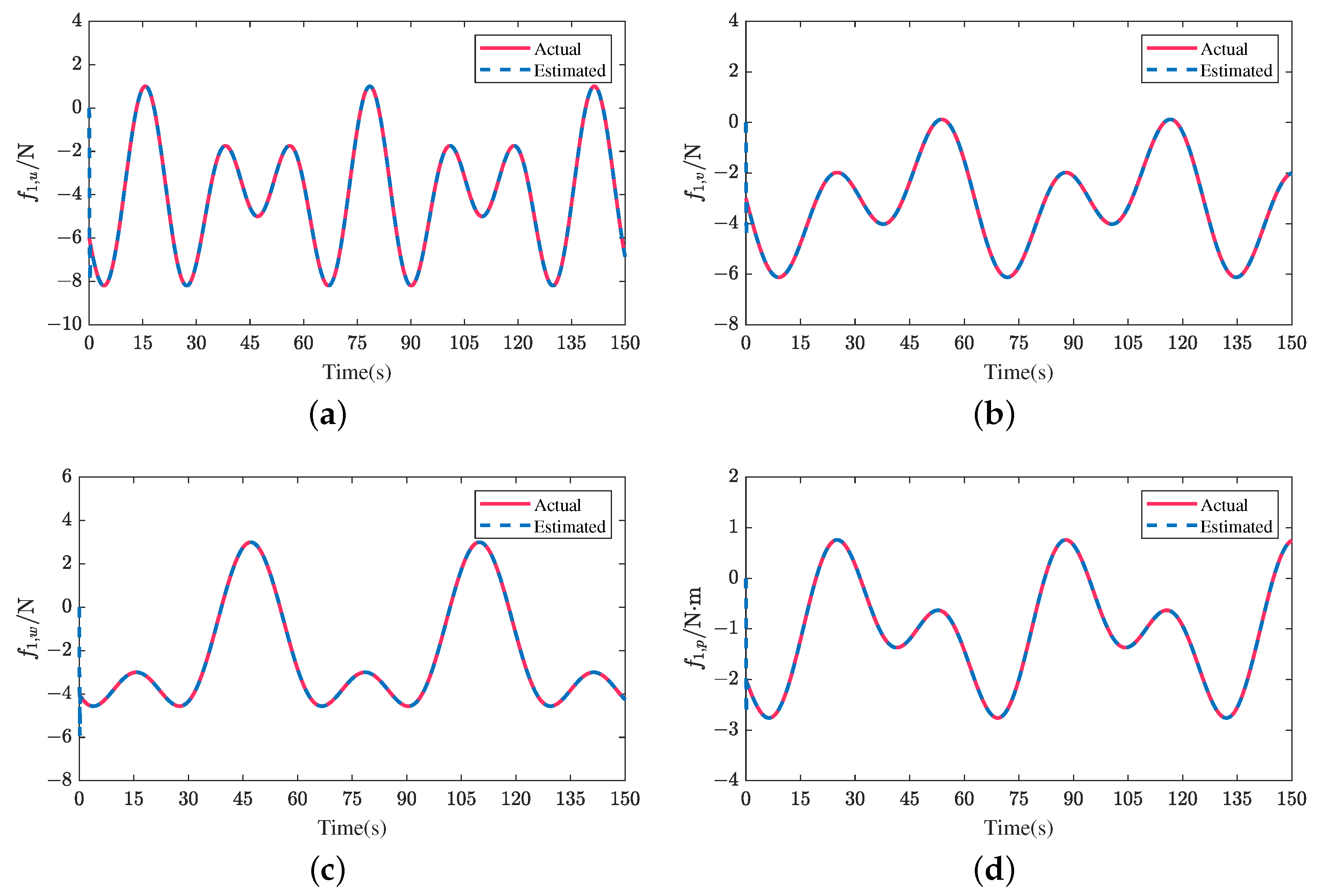
3.1. Design of Adaptive Fixed-Time Disturbance Observer

In order to deal with the external disturbances, an AFxDO is developed for MUVs in this section. To facilitate the disturbance observer design, an auxiliary variable is firstly introduced

$$\begin{array}{c}\hfill {\mathit{e}}_i={\mathit{M}}_i{\mathit{\nu }}_i-{\mathit{\xi }}_i,\end{array}$$

(13)

where $\dot{{\mathit{\xi }}_i}$ is given by

$$\begin{array}{cc}\hfill {\dot{\mathit{\xi }}}_i=& -{\mathit{C}}_i\left({\mathit{\nu }}_i\right){\mathit{\nu }}_i-{\mathit{D}}_i\left({\mathit{\nu }}_i\right){\mathit{\nu }}_i-{\mathit{g}}_i\left({\mathit{\eta }}_i\right)+{\mathit{\tau }}_i\hfill \\ \hfill & +{\mathit{K}}_{10}\mathit{sig}{\left({\mathit{e}}_i\right)}^{2{\alpha }_0-1}+{\mathit{K}}_{20}\mathit{sig}{\left({\mathit{e}}_i\right)}^{2{\beta }_0-1}+\widehat{\gamma }\frac{{\mathit{e}}_i}{\parallel {\mathit{e}}_i\parallel },\hfill \end{array}$$

(14)

where ${\alpha }_0,{\beta }_0,$ are positive design parameters that satisfy $\frac{1}{2}<{\alpha }_0<1$, ${\beta }_0>1$, ${\mathit{K}}_{10}=\mathrm{diag}\left[k_{10,1},k_{10,2},\cdots ,k_{10,6}\right]$, ${\mathit{K}}_{20}=\mathrm{diag}\left[k_{20,1},k_{20,2},\cdots ,k_{20,6}\right]$ are positive definite design matrices and $\widehat{\gamma }>0$ is the estimation of $\gamma$.

Theorem 1. 

Considering the nonlinear uncertain dynamic model of underwater vehicle i given in (1) under Assumption 2, if the AFxDO and the adaptive parameter estimation strategy are designed as

$$\begin{array}{cc}\hfill {\widehat{\mathit{f}}}_i=& {\mathit{K}}_{10}\mathit{sig}{\left({\mathit{e}}_i\right)}^{2{\alpha }_0-1}+{\mathit{K}}_{20}\mathit{sig}{\left({\mathit{e}}_i\right)}^{2{\beta }_0-1}+\widehat{\gamma }\frac{{\mathit{e}}_i}{\parallel {\mathit{e}}_i\parallel },\hfill \end{array}$$

(15)

$$\begin{array}{cc}\hfill {\dot{\widehat{\gamma }}}_i=& {\lambda }_0\parallel {\mathit{e}}_i\parallel -{\lambda }_1{\widehat{\gamma }}_i-{\lambda }_2{\widehat{\gamma }}_i^{2{\beta }_0-1},\hfill \end{array}$$

(16)

where ${\lambda }_0,{\lambda }_1,{\lambda }_2$ are positive constants, then the estimation ${\widehat{\mathit{f}}}_i$ will be stabilized to a small region around ${\mathit{f}}_i$ within a fixed time.

Proof. 

Choose a Lyapunov function candidate as

$$\begin{array}{c}\hfill V_0=\frac{1}{2}{\mathit{e}}_i^T{\mathit{e}}_i+\frac{1}{2{\lambda }_0}{\tilde{\gamma }}_i^2,\end{array}$$

(17)

where ${\tilde{\gamma }}_i={\gamma }_i-{\widehat{\gamma }}_i$ is the estimation error.

Differentiating $V_0$ with respect to time yields

$$\begin{array}{cc}\hfill {\dot{V}}_0=& {\mathit{e}}_i^T\left({\mathit{f}}_i-{\mathit{K}}_{10}\mathit{sig}{\left({\mathit{e}}_i\right)}^{2{\alpha }_0-1}-{\mathit{K}}_{20}\mathit{sig}{\left({\mathit{e}}_i\right)}^{2{\beta }_0-1}-\widehat{\gamma }\frac{{\mathit{e}}_i}{\parallel {\mathit{e}}_i\parallel }\right)-\frac{1}{{\lambda }_0}{\tilde{\gamma }}_i{\dot{\widehat{\gamma }}}_i\hfill \\ \hfill =& -\sum _{\rho =1}^6\left(k_{10,\rho }{e}_{i,\rho }^{2{\alpha }_0}+k_{20,\rho }{e}_{i,\rho }^{2{\beta }_0}\right)+{\mathit{e}}_i^T{\mathit{f}}_i-{\widehat{\gamma }}_i\parallel {\mathit{e}}_i\parallel -\frac{1}{{\lambda }_0}{\tilde{\gamma }}_i{\dot{\widehat{\gamma }}}_i\hfill \\ \hfill \le & -\sum _{\rho =1}^6\left(k_{10,\rho }{e}_{i,\rho }^{2{\alpha }_0}+k_{20,\rho }{e}_{i,\rho }^{2{\beta }_0}\right)+\frac{1}{{\lambda }_0}\tilde{\gamma }\left({\lambda }_0\parallel {\mathit{e}}_i\parallel -{\dot{\widehat{\gamma }}}_i\right).\hfill \end{array}$$

(18)

Substituting the adaptive law (16) into (18), we can obtain

$$\begin{array}{cc}\hfill {\dot{V}}_0\le & -\sum _{\rho =1}^6\left(k_{10,\rho }{e}_{i,\rho }^{2{\alpha }_0}+k_{20,\rho }{e}_{i,\rho }^{2{\beta }_0}\right)+\frac{{\lambda }_1}{{\lambda }_0}{\tilde{\gamma }}_i{\widehat{\gamma }}_i+\frac{{\lambda }_2}{{\lambda }_0}{\tilde{\gamma }}_i{\widehat{\gamma }}_i^{2{\beta }_0-1}.\hfill \end{array}$$

(19)

According to Lemma 3 and the definition of ${\tilde{\gamma }}_i$, we can obtain

$$\begin{array}{c}\hfill {\tilde{\gamma }}_i{\widehat{\gamma }}_i^{2{\beta }_0-1}={\tilde{\gamma }}_i{({\gamma }_i-{\tilde{\gamma }}_i)}^{2{\beta }_0-1}\le \frac{2{\beta }_0-1}{2{\beta }_0}\left({\gamma }_i^{2{\beta }_0}-{\tilde{\gamma }}_i^{2{\beta }_0}\right).\end{array}$$

(20)

By utilizing Lemma 4, let $x=\frac{{\tilde{\gamma }}_i^2}{2{\lambda }_0}$, $y=1$, $a={\alpha }_0$, $b=1-{\alpha }_0$ and $c=1/{\alpha }_0$, then we have

$$\begin{array}{c}\hfill {\left(\frac{{\tilde{\gamma }}_i^2}{2{\lambda }_0}\right)}^{{\alpha }_0}\le \frac{{\tilde{\gamma }}_i^2}{2{\lambda }_0}+(1-{\alpha }_0){\alpha }_0^{\frac{{\alpha }_0}{1-{\alpha }_0}}.\end{array}$$

(21)

Substituting (20) and (21) into (19), we have

$$\begin{array}{cc}\hfill {\dot{V}}_0\le & -\sum _{\rho =1}^6\left(k_{10,\rho }{e}_{i,\rho }^{2{\alpha }_0}+k_{20,\rho }{e}_{i,\rho }^{2{\beta }_0}\right)+\frac{{\lambda }_1}{{\lambda }_0}\left(-\frac{1}{2}{\tilde{\gamma }}_i^2+\frac{1}{2}{\gamma }_i^2\right)+\frac{{\lambda }_2(2{\beta }_0-1)}{2{\beta }_0{\lambda }_0}\left({\gamma }_i^{2{\beta }_0}-{\tilde{\gamma }}_i^{2{\beta }_0}\right)\hfill \\ \hfill \le & -\sum _{\rho =1}^6\left(k_{10,\rho }{e}_{i,\rho }^{2{\alpha }_0}+k_{20,\rho }{e}_{i,\rho }^{2{\beta }_0}\right)-\frac{2^{{\beta }_0}{\lambda }_0^{{\beta }_0-1}{\lambda }_2(2{\beta }_0-1)}{2{\beta }_0}{\left(\frac{{\tilde{\gamma }}_i^2}{2{\lambda }_0}\right)}^{{\beta }_0}\hfill \\ \hfill & -\frac{{\lambda }_1}{2{\lambda }_0}{\tilde{\gamma }}_i^2+\frac{{\lambda }_1}{2{\lambda }_0}{\gamma }_i^2+\frac{{\lambda }_2(2{\beta }_0-1)}{2{\beta }_0{\lambda }_0}{\gamma }_i^{2{\beta }_0}\hfill \\ \hfill \le & -{\sigma }_{min}\left({\mathit{K}}_{10}\right)\sum _{\rho =1}^6{\left(e_{i,\rho }^2\right)}^{{\alpha }_0}-{\sigma }_{min}\left({\mathit{K}}_{20}\right)\sum _{\rho =1}^6{\left(e_{i,\rho }^2\right)}^{{\beta }_0}-{\lambda }_1{\left(\frac{{\tilde{\gamma }}_i^2}{2{\lambda }_0}\right)}^{{\alpha }_0}+\frac{{\lambda }_1{\gamma }_i^2}{2{\lambda }_0}\hfill \\ \hfill & -\frac{{\left(2{\lambda }_0\right)}^{{\beta }_0-1}{\lambda }_2(2{\beta }_0-1)}{{\beta }_0}{\left(\frac{{\tilde{\gamma }}_i^2}{2{\lambda }_0}\right)}^{{\beta }_0}+\frac{{\lambda }_2(2{\beta }_0-1)}{2{\beta }_0{\lambda }_0}{\gamma }_i^{2{\beta }_0}+{\lambda }_1(1-{\alpha }_0){\alpha }_0^{\frac{{\alpha }_0}{1-{\alpha }_0}}\hfill \\ \hfill \le & -min\left\{{\sigma }_{min}\left({\mathit{K}}_{10}\right)2^{{\alpha }_0},{\lambda }_1\right\}\left({\left(\frac{{\mathit{e}}_i^T{\mathit{e}}_i}{2}\right)}^{{\alpha }_0}+{\left(\frac{{\tilde{\gamma }}_i^2}{2{\lambda }_0}\right)}^{{\alpha }_0}\right)\hfill \\ \hfill & -min\left\{2{\sigma }_{min}\left({\mathit{K}}_{20}\right)3^{1-{\beta }_0},\frac{{\left(2{\lambda }_0\right)}^{{\beta }_0-1}{\lambda }_2(2{\beta }_0-1)}{{\beta }_0}\right\}\left({\left(\frac{{\mathit{e}}_i^T{\mathit{e}}_i}{2}\right)}^{{\beta }_0}+{\left(\frac{{\tilde{\gamma }}_i^2}{2{\lambda }_0}\right)}^{{\beta }_0}\right)+{\Omega }_0\hfill \\ \hfill \le & -A_0{V}_0^{{\alpha }_0}-B_0{V}_0^{{\beta }_0}+{\Omega }_0,\hfill \end{array}$$

(22)

where

$$\begin{array}{cc}\hfill & A_0=min\left\{{\sigma }_{min}\left({\mathit{K}}_{10}\right)2^{{\alpha }_0},{\lambda }_1\right\},\hfill \\ \hfill & B_0=2^{1-{\beta }_0}min\left\{2{\sigma }_{min}\left({\mathit{K}}_{20}\right)3^{1-{\beta }_0},\frac{{\left(2{\lambda }_0\right)}^{{\beta }_0-1}{\lambda }_2(2{\beta }_0-1)}{{\beta }_0}\right\},\hfill \\ \hfill & {\Omega }_0=\frac{{\lambda }_1{\gamma }_i^2}{2{\lambda }_0}+\frac{{\lambda }_2(2{\beta }_0-1)}{2{\beta }_0{\lambda }_0}{\gamma }_i^{2{\beta }_0}+{\lambda }_1(1-{\alpha }_0){\alpha }_0^{\frac{{\alpha }_0}{1-{\alpha }_0}}.\hfill \end{array}$$

Since (22) satisfies Lemma 2, system (17) is, therefore, proven to be practical fixed-time stable, and the settling time can be expressed as

$$\begin{array}{c}\hfill t_0\le T_{\max }=\frac{1}{{\omega }_0{A}_0(1-{\alpha }_0)}+\frac{1}{{\omega }_0{B}_0({\beta }_0-1)},\end{array}$$

(23)

where $0<{\omega }_0<1$. If ${\tilde{\gamma }}_i=0$, then according to (17), we have

$$\begin{array}{c}\hfill {\dot{V}}_0={\mathit{e}}_i^T\dot{{\mathit{e}}_i}\le -\sum _{\rho =1}^6\left(k_{10,\rho }{e}_{i,\rho }^{2{\alpha }_0}+k_{20,\rho }{e}_{i,\rho }^{2{\beta }_0}\right).\end{array}$$

(24)

According to Lemma 1, the auxiliary variable ${\mathit{e}}_i$ will be stabilized to zero in a fixed time when ${\tilde{\gamma }}_i=0$. Thus, its derivative ${\dot{\mathit{e}}}_i$ will also converge to zero in fixed time. From (13)–(15), we have ${\tilde{\mathit{f}}}_i={\mathit{f}}_i-{\widehat{\mathit{f}}}_i={\mathit{M}}_i{\dot{\mathit{\nu }}}_i-{\dot{\xi }}_i={\dot{\mathit{e}}}_i$. Therefore, ${\mathit{f}}_i={\widehat{\mathit{f}}}_i$ when ${\tilde{\gamma }}_i=0$. For the case ${\tilde{\gamma }}_i\ne 0$, it is easy to obtain ${\tilde{\mathit{f}}}_i={\mathit{f}}_i-{\widehat{\mathit{f}}}_i=\left({\gamma }_i-{\widehat{\gamma }}_i\right)\frac{{\mathit{e}}_i}{\parallel {\mathit{e}}_i\parallel }={\tilde{\gamma }}_i\frac{{\mathit{e}}_i}{\parallel {\mathit{e}}_i\parallel }$. From (22), ${\tilde{\gamma }}_i$ will converge to the neighborhood of the origin when $t>t_0$. Thus, ${\widehat{\mathit{f}}}_i$ will converge to the neighborhood of ${\mathit{f}}_i$ when $t>t_0$. □

Remark 2. 

Different from the asymptotic and finite-time convergent disturbance observers, the developed AFxDO guarantees the fixed-time convergence property of observation errors, i.e., the convergence time is upper-bounded by an a priori value, irrespective of initial conditions. Additionally, the developed AFxDO eliminates the need for prior knowledge of the upper bound value of external disturbances, which is useful for practical applications.

3.2. Design of Distributed Event-Triggered Fixed-Time Formation Tracking Controller

The block diagram of the proposed control strategy is shown in Figure 2. As seen from Figure 2, a distributed event-triggered fixed-time backstepping controller is proposed for the formation tracking control of MUVs based on the developed AFxDO. The proposed formation tracking control strategy has strong robustness, a fast convergence rate, and reduces the communication burden. The details are as follows.

For underwater vehicle i, underwater vehicle j is supposed to be its neighbor. Define the formation tracking error ${\tilde{\mathit{\eta }}}_i\in {\mathbb{R}}^6$ of underwater vehicle i as

$$\begin{array}{cc}\hfill {\tilde{\mathit{\eta }}}_i=& \sum _{j=0}^n{a}_{ij}\left({\mathit{\eta }}_i-{\mathit{\eta }}_j-\Delta {\mathit{\eta }}_{ij}\right),\hfill \end{array}$$

(25)

where ${\tilde{\mathit{\eta }}}_i={\left[{\tilde{x}}_i,{\tilde{y}}_i,{\tilde{z}}_i,{\tilde{\varphi }}_i,{\tilde{\theta }}_i,{\tilde{\psi }}_i\right]}^T$ and $\Delta {\mathit{\eta }}_{ij}={\left[\Delta x_{ij},\Delta y_{ij},\Delta z_{ij},\Delta {\varphi }_{ij},\Delta {\theta }_{ij},\Delta {\psi }_{ij}\right]}^T$ is the desired formation pattern for i and j, $i\ne 0$.

The time derivative of (25) yields

$$\begin{array}{cc}\hfill {\dot{\tilde{\mathit{\eta }}}}_i=& \sum _{j=0}^n{a}_{ij}\left({\mathit{J}}_i\left({\mathit{\eta }}_i\right){\mathit{\nu }}_i-{\dot{\mathit{\eta }}}_j\right).\hfill \end{array}$$

(26)

To guarantee the fixed-time convergence of the formation tracking error ${\tilde{\mathit{\eta }}}_i$ of underwater vehicle i, the virtual control law ${\mathit{\chi }}_{c,i}$ can be designed as follows:

$$\begin{array}{cc}\hfill {\mathit{\chi }}_{c,i}=& \frac{1}{h_i}{\mathit{J}}_i^{-1}\left({\mathit{\eta }}_i\right)\left(\sum _{j=0}^n{a}_{ij}{\dot{\mathit{\eta }}}_j-{\mathit{K}}_{11}\mathit{sig}{\left({\tilde{\mathit{\eta }}}_i\right)}^{2{\alpha }_1-1}-{\mathit{K}}_{21}\mathit{sig}{\left({\tilde{\mathit{\eta }}}_i\right)}^{2{\beta }_1-1}\right),\hfill \end{array}$$

(27)

where ${\alpha }_1,{\beta }_1,$ are positive design parameters that satisfy $\frac{1}{2}<{\alpha }_1<1,{\beta }_1>1$, and ${\mathit{K}}_{11}=\mathrm{diag}\left[k_{11,1},k_{11,2},\cdots ,k_{11,6}\right]$, ${\mathit{K}}_{21}=\mathrm{diag}\left[k_{21,1},k_{21,2},\cdots ,k_{21,6}\right]$ are positive definite design matrices.

To deal with the “explosion of complexity” issue that is inherent in the traditional backstepping control, let ${\mathit{\chi }}_{c,i}$ pass through the following first-order nonlinear filter

$$\begin{array}{cc}\hfill \kappa {\dot{\mathit{\chi }}}_{d,i}=& -\mathit{sig}{({\mathit{\chi }}_{d,i}-{\mathit{\chi }}_{c,i})}^{2{\alpha }_1-1}-\mathit{sig}{({\mathit{\chi }}_{d,i}-{\mathit{\chi }}_{c,i})}^{2{\beta }_1-1},\hfill \end{array}$$

(28)

where ${\mathit{\chi }}_{d,i}$ is the filtered virtual control scheme and $\kappa >0$ is the designed parameter. According to (28), the differential term ${\dot{\mathit{\chi }}}_{d,i}$ is directly obtained to replace the complicated differential term ${\dot{\mathit{\chi }}}_{c,i}$ required in the traditional backstepping control. It is noteworthy that the filter employed here is nonlinear rather than linear since the linear filter cannot achieve the fixed-time convergence property of the overall system.

The velocity tracking error ${\tilde{\mathit{\nu }}}_i\in {\mathbb{R}}^6$ is defined as

$$\begin{array}{cc}\hfill {\tilde{\mathit{\nu }}}_i=& {\mathit{\nu }}_i-{\mathit{\chi }}_{d,i},\hfill \end{array}$$

(29)

Differentiating (29) with respect to time and substituting (1) into it, we have

$$\begin{array}{cc}\hfill {\dot{\tilde{\mathit{\nu }}}}_i=& {\mathit{M}}_i^{-1}\left(-{\mathit{C}}_i\left({\mathit{\nu }}_i\right){\mathit{\nu }}_i-{\mathit{D}}_i\left({\mathit{\nu }}_i\right){\mathit{\nu }}_i-{\mathit{g}}_i\left({\mathit{\eta }}_i\right)+{\mathit{\tau }}_i+{\mathit{f}}_i\right)-{\dot{\mathit{\chi }}}_{d,i},\hfill \end{array}$$

(30)

To achieve the fixed-time convergence of the velocity tracking error ${\tilde{\mathit{\nu }}}_i$ and enhance the system’s robustness against external disturbances, the AFxDO-based distributed event-triggered fixed-time formation tracking control scheme for the underwater vehicle i can be designed as

$$\begin{array}{cc}\hfill {\overline{\mathit{\tau }}}_i=& {\mathit{C}}_i\left({\mathit{\nu }}_i\right){\mathit{\nu }}_i+{\mathit{D}}_i\left({\mathit{\nu }}_i\right){\mathit{\nu }}_i+{\mathit{g}}_i\left({\mathit{\eta }}_i\right)-{\widehat{\mathit{f}}}_i+{\mathit{M}}_i{\dot{\mathit{\chi }}}_{d,i}\hfill \\ \hfill & -{\mathit{K}}_{12}\mathit{sig}{\left({\tilde{\mathit{\nu }}}_i\right)}^{2{\alpha }_1-1}-{\mathit{K}}_{22}\mathit{sig}{\left({\tilde{\mathit{\nu }}}_i\right)}^{2{\beta }_1-1}-{\mu }_{2}tanh\left(\frac{{\tilde{\mathit{\nu }}}_i}{{\varrho }_i}\right)-\frac{{\tilde{\mathit{\nu }}}_i{\parallel {\tilde{\mathit{\nu }}}_i\parallel }^2}{2},\hfill \end{array}$$

(31)

with the triggering event condition given as

$$\begin{array}{c}\hfill \left\{\begin{array}{c}{\mathit{\tau }}_i\left(t\right)={\overline{\mathit{\tau }}}_i\left(t_{i,m}\right),t\in \left[t_{i,m},t_{i,m+1}\right),\hfill \\ {\mathit{t}}_{i,m+1}=inf\left\{t>t_{i,m}\left|\parallel {\tilde{\mathit{\tau }}}_i\left(t\right)\parallel \ge {\mu }_1\parallel {\tilde{\mathit{\nu }}}_i\left(t\right)\parallel +{\mu }_2\right.\right\}\hfill \end{array}\right.\end{array}$$

(32)

where ${\mu }_1,{\mu }_2$ are positive design parameters, ${\mathit{K}}_{12}=\mathrm{diag}\left[k_{12,1},k_{12,2},\cdots ,k_{12,6}\right]$, ${\mathit{K}}_{22}=\mathrm{diag}\left[k_{22,1},k_{22,2},\cdots ,k_{22,6}\right]$ are positive definite design matrices, $t_{i,m}$ ($m\in {\mathbb{Z}}^{+}$) is the triggering time of the control law for underwater vehicle i, and ${\tilde{\mathit{\tau }}}_i\left(t\right)={\overline{\mathit{\tau }}}_i\left(t\right)-{\mathit{\tau }}_i\left(t\right)$. Equation (32) indicates that when the triggering condition $\parallel {\tilde{\mathit{\tau }}}_i\parallel \ge {\mu }_1\parallel {\tilde{\mathit{\nu }}}_i\parallel +{\mu }_2$ is satisfied, the control input ${\mathit{\tau }}_i$ updates its value at $t_{i,m+1}$, and is then set to ${\overline{\mathit{\tau }}}_i$ during $t\in \left[t_{i,m},t_{i,m+1}\right)$.

Theorem 2. 

Considering the MUV system given in (1) under Assumptions 1 and 2, if the distributed fixed-time control scheme is designed as (31), based on the virtual control law (27), the first-order nonlinear filter (28), the event-triggering law (32), and the AFxDO (15), then the formation tracking control can be achieved for the MUV system, and all signals of the MUV system are practical fixed-time stable. Additionally, the Zeno behavior can be excluded.

Proof. 

The proof of Theorem 2 depends on the premise that the disturbance estimation error ${\tilde{\mathit{f}}}_i$ is stabilized toward a small neighborhood of the origin in fixed time. Actually, this premise can be achieved in Theorem 1, where the AFxDO is designed to estimate the external disturbances ${\mathit{f}}_i$ in a fixed time $t_0$. Therefore, we can assume that when $t>t_0$, ${\tilde{\mathit{f}}}_i$ converges to a small region of the origin, and there exists a small positive constant ${\delta }_i$, satisfying $\parallel {\tilde{\mathit{f}}}_i\parallel \le {\delta }_i$. Then, we consider the following Lyapunov function candidate

$$\begin{array}{c}\hfill V_1=\frac{1}{2}{\tilde{\mathit{\eta }}}_i^T{\tilde{\mathit{\eta }}}_i+\frac{1}{2}{\tilde{\mathit{\chi }}}_i^T{\tilde{\mathit{\chi }}}_i+\frac{1}{2}{\tilde{\mathit{\nu }}}_i^T{\mathit{M}}_i{\tilde{\mathit{\nu }}}_i.\end{array}$$

(33)

where ${\tilde{\mathit{\chi }}}_i={\mathit{\chi }}_{d,i}-{\mathit{\chi }}_{c,i}$ is the filtered error.

Differentiating $V_1$ with respective to time, we have

$$\begin{array}{c}\hfill {\dot{V}}_1={\tilde{\mathit{\eta }}}_i^T{\dot{\tilde{\mathit{\eta }}}}_i+{\tilde{\mathit{\chi }}}_i^T{\dot{\tilde{\mathit{\chi }}}}_i+{\tilde{\mathit{\nu }}}_i^T{\mathit{M}}_i{\dot{\tilde{\mathit{\nu }}}}_i.\end{array}$$

(34)

According to (26) and (29), we have

$$\begin{array}{cc}\hfill {\tilde{\mathit{\eta }}}_i^T{\dot{\tilde{\mathit{\eta }}}}_i=& {\tilde{\mathit{\eta }}}_i^T\left(\sum _{j=0}^n{a}_{ij}\left({\mathit{J}}_i\left({\mathit{\eta }}_i\right){\mathit{\nu }}_i-{\dot{\mathit{\eta }}}_j\right)\right)\hfill \\ \hfill =& {\tilde{\mathit{\eta }}}_i^T\left(h_i{\mathit{J}}_i\left({\mathit{\eta }}_i\right)\left({\tilde{\mathit{\chi }}}_i+{\tilde{\mathit{\nu }}}_i+{\mathit{\chi }}_{c,i}\right)-\sum _{j=0}^n{a}_{ij}{\dot{\mathit{\eta }}}_j\right)\hfill \\ \hfill =& -\sum _{\rho =1}^6\left(k_{11,\rho }{\tilde{\eta }}_{i,\rho }^{2{\alpha }_1}+k_{21,\rho }{\tilde{\eta }}_{i,\rho }^{2{\beta }_1}\right)+h_i{\tilde{\mathit{\eta }}}_i^T{\mathit{J}}_i\left({\mathit{\eta }}_i\right)\left({\tilde{\mathit{\chi }}}_i+{\tilde{\mathit{\nu }}}_i\right)\hfill \\ \hfill \le & -\sum _{\rho =1}^6\left(k_{11,\rho }{\tilde{\eta }}_{i,\rho }^{2{\alpha }_1}+k_{21,\rho }{\tilde{\eta }}_{i,\rho }^{2{\beta }_1}\right)+h_i{\overline{J}}_i\left({\tilde{\mathit{\eta }}}_i^T{\tilde{\mathit{\eta }}}_i+\frac{1}{2}{\tilde{\mathit{\chi }}}_i^T{\tilde{\mathit{\chi }}}_i+\frac{1}{2}{\tilde{\mathit{\nu }}}_i^T{\tilde{\mathit{\nu }}}_i\right).\hfill \end{array}$$

(35)

Based on the definition of ${\tilde{\mathit{\chi }}}_i$, its derivative can be expressed as

$$\begin{array}{c}\hfill {\dot{\tilde{\mathit{\chi }}}}_i=-\frac{1}{\kappa }\mathit{sig}{\left({\tilde{\mathit{\chi }}}_i\right)}^{2{\alpha }_1-1}-\frac{1}{\kappa }\mathit{sig}{\left({\tilde{\mathit{\chi }}}_i\right)}^{2{\beta }_1-1}-{\dot{\mathit{\chi }}}_{c,i}.\end{array}$$

(36)

In the light of (27), we can assume that ${\dot{\mathit{\chi }}}_{c,i}$ is bounded, i.e., $\parallel {\dot{\mathit{\chi }}}_{c,i}\parallel <{\varsigma }_i,{\varsigma }_i>0$. Then, we have

$$\begin{array}{cc}\hfill {\tilde{\mathit{\chi }}}_i^T{\dot{\tilde{\mathit{\chi }}}}_i=& -\frac{1}{\kappa }\sum _{\rho =1}^6\left({\tilde{\chi }}_{i,\rho }^{2{\alpha }_1}+{\tilde{\chi }}_{i,\rho }^{2{\beta }_1}\right)-{\tilde{\mathit{\chi }}}_i^T{\dot{\mathit{\chi }}}_{c,i}\hfill \\ \hfill \le & -\frac{1}{\kappa }\sum _{\rho =1}^6\left({\tilde{\chi }}_{i,\rho }^{2{\alpha }_1}+{\tilde{\chi }}_{i,\rho }^{2{\beta }_1}\right)+\parallel {\tilde{\mathit{\chi }}}_i\parallel \parallel {\dot{\mathit{\chi }}}_{c,i}\parallel \hfill \\ \hfill \le & -\frac{1}{\kappa }\sum _{\rho =1}^6\left({\tilde{\chi }}_{i,\rho }^{2{\alpha }_1}+{\tilde{\chi }}_{i,\rho }^{2{\beta }_1}\right)+\frac{1}{2}{\tilde{\mathit{\chi }}}_i^T{\tilde{\mathit{\chi }}}_i+\frac{1}{2}{\varsigma }_i^2.\hfill \end{array}$$

(37)

In view of (30)–(32), we have

$$\begin{array}{cc}\hfill {\tilde{\mathit{\nu }}}_i^T{\mathit{M}}_i{\dot{\tilde{\mathit{\nu }}}}_i=& {\tilde{\mathit{\nu }}}_i^T\left({\tilde{\mathit{f}}}_i-{\tilde{\mathit{\tau }}}_i-{\mathit{K}}_{12}\mathit{sig}{\left({\tilde{\mathit{\nu }}}_i\right)}^{2{\alpha }_1-1}-{\mathit{K}}_{22}\mathit{sig}{\left({\tilde{\mathit{\nu }}}_i\right)}^{2{\beta }_1-1}-{\mu }_{2}tanh\left(\frac{{\tilde{\mathit{\nu }}}_i}{{\varrho }_i}\right)-\frac{{\tilde{\mathit{\nu }}}_i{\parallel {\tilde{\mathit{\nu }}}_i\parallel }^2}{2}\right)\hfill \\ \hfill \le & -\sum _{\rho =1}^6\left(k_{12,\rho }{\tilde{\nu }}_{i,\rho }^{2{\alpha }_1}+k_{22,\rho }{\tilde{\nu }}_{i,\rho }^{2{\beta }_1}\right)+\frac{1}{2}{\tilde{\mathit{\nu }}}_i^T{\tilde{\mathit{\nu }}}_i+\frac{{\delta }_i^2}{2}\hfill \\ \hfill & +\parallel {\tilde{\mathit{\nu }}}_i\parallel \left({\mu }_1\parallel {\tilde{\mathit{\nu }}}_i\parallel +{\mu }_{i,2}\right)-{\mu }_2{\tilde{\mathit{\nu }}}_i^{T}tanh\left(\frac{{\tilde{\mathit{\nu }}}_i}{{\varrho }_i}\right)-\frac{\parallel {\tilde{\mathit{\nu }}}_i{\parallel }^4}{2}\hfill \\ \hfill \le & -\sum _{\rho =1}^6\left(k_{12,\rho }{\tilde{\nu }}_{i,\rho }^{2{\alpha }_1}+k_{22,\rho }{\tilde{\nu }}_{i,\rho }^{2{\beta }_1}\right)+\frac{1}{2}{\tilde{\mathit{\nu }}}_i^T{\tilde{\mathit{\nu }}}_i\hfill \\ \hfill & +{\mu }_2\left(\parallel {\tilde{\mathit{\nu }}}_i\parallel -{\tilde{\mathit{\nu }}}_i^{T}tanh\left(\frac{{\tilde{\mathit{\nu }}}_i}{{\varrho }_i}\right)\right)+\frac{{\delta }_i^2}{2}+\frac{{\mu }_1^2}{2}.\hfill \end{array}$$

(38)

From the definition of ${\tilde{\mathit{\nu }}}_i$ and $tanh\left(\frac{{\tilde{\mathit{\nu }}}_i}{{\varrho }_i}\right)$, and utilizing Lemma 5 yields

$$\begin{array}{c}\hfill \parallel {\tilde{\mathit{\nu }}}_i\parallel -{\tilde{\mathit{\nu }}}_i^{T}tanh\left(\frac{{\tilde{\mathit{\nu }}}_i}{{\varrho }_i}\right)\le \sum _{\rho =1}^6\left(|{\tilde{\nu }}_{i,\rho }|-{\tilde{\nu }}_{i,\rho }tanh\left(\frac{{\tilde{\nu }}_{i,\rho }}{{\varrho }_i}\right)\right)\le 1.671{\varrho }_i.\end{array}$$

(39)

Substituting (35)–(39) into (34), we have

$$\begin{array}{cc}\hfill {\dot{V}}_1\le & -\sum _{\rho =1}^6\left(k_{11,\rho }{\tilde{\eta }}_{i,\rho }^{2{\alpha }_1}+k_{21,\rho }{\tilde{\eta }}_{i,\rho }^{2{\beta }_1}\right)+h_i{\overline{J}}_i\left({\tilde{\mathit{\eta }}}_i^T{\tilde{\mathit{\eta }}}_i+\frac{1}{2}{\tilde{\mathit{\chi }}}_i^T{\tilde{\mathit{\chi }}}_i+\frac{1}{2}{\tilde{\mathit{\nu }}}_i^T{\tilde{\mathit{\nu }}}_i\right)-\frac{1}{\kappa }\sum _{\rho =1}^6\left({\tilde{\chi }}_{i,\rho }^{2{\alpha }_1}+{\tilde{\chi }}_{i,\rho }^{2{\beta }_1}\right)\hfill \\ \hfill & +\frac{1}{2}{\tilde{\mathit{\chi }}}_i^T{\tilde{\mathit{\chi }}}_i+\frac{1}{2}{\varsigma }_i^2-\sum _{\rho =1}^6\left(k_{12,\rho }{\tilde{\nu }}_{i,\rho }^{2{\alpha }_1}+k_{22,\rho }{\tilde{\nu }}_{i,\rho }^{2{\beta }_1}\right)+\frac{1}{2}{\tilde{\mathit{\nu }}}_i^T{\tilde{\mathit{\nu }}}_i+1.671{\mu }_2{\varrho }_i+\frac{{\delta }_i^2}{2}+\frac{{\mu }_1^2}{2}\hfill \\ \hfill & +\frac{1+h_i{\overline{J}}_i}{2}{\tilde{\mathit{\chi }}}_i^T{\tilde{\mathit{\chi }}}_i+\frac{1+h_i{\overline{J}}_i}{2}{\tilde{\mathit{\nu }}}_i^T{\tilde{\mathit{\nu }}}_i+1.671{\mu }_2{\varrho }_i+\frac{{\delta }_i^2}{2}+\frac{{\mu }_1^2}{2}+\frac{1}{2}{\varsigma }_i^2\hfill \\ \hfill \le & -\sum _{\rho =1}^6\left(\left(k_{11,\rho }-h_i{\overline{J}}_i\right){\tilde{\eta }}_{i,\rho }^{2{\alpha }_1}+\left(\frac{1}{\kappa }-\frac{1}{2}-\frac{h_i{\overline{J}}_i}{2}\right){\tilde{\chi }}_{i,\rho }^{2{\alpha }_1}+\left(k_{12,\rho }-\frac{1}{2}-\frac{h_i{\overline{J}}_i}{2}\right){\tilde{\nu }}_{i,\rho }^{2{\alpha }_1}\right)\hfill \\ \hfill & -\sum _{\rho =1}^6\left(\left(k_{21,\rho }-h_i{\overline{J}}_i\right){\tilde{\eta }}_{i,\rho }^{2{\beta }_1}+\left(\frac{1}{\kappa }-\frac{1}{2}-\frac{h_i{\overline{J}}_i}{2}\right){\tilde{\chi }}_{i,\rho }^{2{\beta }_1}+\left(k_{22,\rho }-\frac{1}{2}-\frac{h_i{\overline{J}}_i}{2}\right){\tilde{\nu }}_{i,\rho }^{2{\beta }_1}\right)\hfill \\ \hfill & +1.671{\mu }_2{\varrho }_i+\frac{{\delta }_i^2}{2}+\frac{{\mu }_1^2}{2}+\frac{1}{2}{\varsigma }_i^2\hfill \\ \hfill \le & -\left({\sigma }_{min}\left({\mathit{K}}_{11}\right)-h_i{\overline{J}}_i\right){\left({\tilde{\mathit{\eta }}}_i^T{\tilde{\mathit{\eta }}}_i\right)}^{{\alpha }_1}-\left(\frac{1}{\kappa }-\frac{1}{2}-\frac{h_i{\overline{J}}_i}{2}\right){\left({\tilde{\mathit{\chi }}}_i^T{\tilde{\mathit{\chi }}}_i\right)}^{{\alpha }_1}\hfill \\ \hfill & -\frac{{\sigma }_{min}\left({\mathit{K}}_{12}\right)-\frac{1}{2}-\frac{h_i{\overline{J}}_i}{2}}{{\sigma }_{max}^{{\alpha }_1}\left(\mathit{M}\right)}{\left({\tilde{\mathit{\eta }}}_i^T\mathit{M}{\tilde{\mathit{\eta }}}_i\right)}^{{\alpha }_1}+6^{1-{\beta }_1}\left(-\left({\sigma }_{min}\left({\mathit{K}}_{21}\right)-h_i{\overline{J}}_i\right){\left({\tilde{\mathit{\eta }}}_i^T{\tilde{\mathit{\eta }}}_i\right)}^{{\beta }_1}\right.\hfill \\ \hfill & \left.-\left(\frac{1}{\kappa }-\frac{1}{2}-\frac{h_i{\overline{J}}_i}{2}\right){\left({\tilde{\mathit{\chi }}}_i^T{\tilde{\mathit{\chi }}}_i\right)}^{{\beta }_1}-\frac{{\sigma }_{min}\left({\mathit{K}}_{22}\right)-\frac{1}{2}-\frac{h_i{\overline{J}}_i}{2}}{{\sigma }_{max}^{{\beta }_1}\left(\mathit{M}\right)}{\left({\tilde{\mathit{\eta }}}_i^T\mathit{M}{\tilde{\mathit{\eta }}}_i\right)}^{{\beta }_1}\right)\hfill \\ \hfill & +1.671{\mu }_2{\varrho }_i+\frac{{\delta }_i^2}{2}+\frac{{\mu }_1^2}{2}+\frac{1}{2}{\varsigma }_i^2\hfill \\ \hfill \le & -2^{{\alpha }_1}{\overline{A}}_1\left({\left(\frac{1}{2}{\tilde{\mathit{\eta }}}_i^T{\tilde{\mathit{\eta }}}_i\right)}^{{\alpha }_1}+{\left(\frac{1}{2}{\tilde{\mathit{\chi }}}_i^T{\tilde{\mathit{\chi }}}_i\right)}^{{\alpha }_1}+{\left(\frac{1}{2}{\tilde{\mathit{\nu }}}_i^T{\mathit{M}}_i{\tilde{\mathit{\nu }}}_i\right)}^{{\alpha }_1}\right)\hfill \\ \hfill & -6^{1-{\beta }_1}{\overline{B}}_1\left({\left(\frac{1}{2}{\tilde{\mathit{\eta }}}_i^T{\tilde{\mathit{\eta }}}_i\right)}^{{\beta }_1}+{\left(\frac{1}{2}{\tilde{\mathit{\chi }}}_i^T{\tilde{\mathit{\chi }}}_i\right)}^{{\beta }_1}+{\left(\frac{1}{2}{\tilde{\mathit{\nu }}}_i^T{\mathit{M}}_i{\tilde{\mathit{\nu }}}_i\right)}^{{\beta }_1}\right)+{\Omega }_1\hfill \\ \hfill =& -A_1{V}_1^{{\alpha }_1}-B_1{V}_1^{{\beta }_1}+{\Omega }_1,\hfill \end{array}$$

(40)

where $A_1=2^{{\alpha }_1}{\overline{A}}_1$, ${\overline{A}}_1=min\left\{{\sigma }_{min}\left({\mathit{K}}_{11}\right)-h_i{\overline{J}}_i,\frac{1}{\kappa }-\frac{1}{2}-\frac{h_i{\overline{J}}_i}{2},\frac{{\sigma }_{min}\left({\mathit{K}}_{12}\right)-\frac{1}{2}-\frac{h_i{\overline{J}}_i}{2}}{{\sigma }_{max}^{{\alpha }_1}\left(\mathit{M}\right)}\right\}$, $B_1={18}^{1-{\beta }_1}{\overline{B}}_1$, ${\overline{B}}_1=min\left\{{\sigma }_{min}\left({\mathit{K}}_{21}\right)-h_i{\overline{J}}_i,\frac{1}{\kappa }-\frac{1}{2}-\frac{h_i{\overline{J}}_i}{2},\frac{{\sigma }_{min}\left({\mathit{K}}_{22}\right)-\frac{1}{2}-\frac{h_i{\overline{J}}_i}{2}}{{\sigma }_{max}^{{\beta }_1}\left(\mathit{M}\right)}\right\}$, ${\Omega }_1=1.671{\mu }_2{\varrho }_i$$+\frac{{\delta }_i^2}{2}+\frac{{\mu }_1^2}{2}+\frac{1}{2}{\varsigma }_i^2$.

According to Lemma 2, system (33) is practical fixed stable, and the tracking errors of the MUV system converge to an arbitrarily small region of the origin within a fixed time, which is determined by

$$\begin{array}{c}\hfill t_1\le T_{\max }=\frac{1}{{\omega }_1{A}_1(1-{\alpha }_1)}+\frac{1}{{\omega }_1{B}_1({\beta }_1-1)}.\end{array}$$

(41)

To avoid the Zeno behavior, we show that minimal inter-event times $t_i^{*}$ exist, which satisfy $\left(t_{i,m+1}-t_{i,m}\right)>t_i^{*}$ for $m\in {\mathbb{Z}}^{+}$.

For $t\in [t_{i,m},t_{i,m+1})$, we have ${\dot{\mathit{\tau }}}_i\left(t\right)=0$, then taking the time derivative of the measurement error ${\tilde{\mathit{\tau }}}_i\left(t\right)$ yields

$$\begin{array}{c}\hfill \frac{d}{dt}\parallel {\tilde{\mathit{\tau }}}_i\left(t\right)\parallel =\frac{d}{dt}{\left[{\tilde{\mathit{\tau }}}_i^T\left(t\right){\tilde{\mathit{\tau }}}_i\left(t\right)\right]}^{\frac{1}{2}}=\frac{{\tilde{\mathit{\tau }}}_i^T\left(t\right){\dot{\tilde{\mathit{\tau }}}}_i\left(t\right)}{\parallel {\tilde{\mathit{\tau }}}_i\left(t\right)\parallel }\le ∥\frac{d}{dt}{\overline{\mathit{\tau }}}_i\left(t\right)∥.\end{array}$$

(42)

Since all the signals of the closed-loop MUV system are bounded, there is a positive constant ${\epsilon }_i$, satisfying $∥\frac{d}{dt}{\overline{\mathit{\tau }}}_i\left(t\right)∥<{\epsilon }_i$. Then, integrating (42) over $t\in [t_{i,m},t_{i,m+1})$ and employing the event-triggering condition given in (32), we have

$$\begin{array}{c}\hfill t_{i,m+1}-t_{i,m}\ge \frac{\parallel {\tilde{\mathit{\tau }}}_i\left(t\right)\parallel }{{\epsilon }_i}\ge \frac{{\mu }_1\parallel {\tilde{\mathit{\nu }}}_i\parallel +{\mu }_2}{{\epsilon }_i}\ge \frac{{\mu }_2}{{\epsilon }_i}=t_i^{*}.\end{array}$$

(43)

Therefore, it holds that $\left(t_{i,m+1}-t_{i,m}\right)>t_i^{*}$ with $t_i^{*}=\frac{{\mu }_2}{{\epsilon }_i}$. □

Remark 3. 

Different from the finite-time methods [17,19,20,21,22], in this paper, the designed distributed event-triggered fixed-time backstepping control scheme can make the formation tracking errors converge to the origin within fixed-time independent of initial conditions, while the signal transmission frequencies are effectively reduced.

Remark 4. 

Although the control design for MUVs subjected to external disturbances is investigated, the proposed control scheme can be easily extended to handle other engineering systems [42,43,44,45]. In addition, the developed control scheme is based on the model. The accurate underwater vehicle model will lead to better control performance. Therefore, some advanced parameter estimation algorithms [46,47,48,49] can be used to establish an accurate model.

Remark 5. 

The parameters of the proposed control scheme should be selected according to the following adjustment guidelines: (1) Controller parameters—increasing ${\mathit{K}}_{11},{\mathit{K}}_{21},{\mathit{K}}_{12},{\mathit{K}}_{22},{\beta }_1,{\mu }_1,{\mu }_2$ and decreasing ${\alpha }_1$ will improve the convergence rate, reduce the system tracking errors, and prolong the inter-event time. However, too large ${\mathit{K}}_{11},{\mathit{K}}_{10},{\mathit{K}}_{20},{\mathit{K}}_{22},{\beta }_1,{\mu }_1,{\mu }_2$, and too small ${\alpha }_1$ will result in severe input saturation and high-frequency changes in the vehicle states. (2) Observer parameters—increasing ${\mathit{K}}_{11},{\mathit{K}}_{21},{\lambda }_0,{\beta }_0$ and decreasing ${\lambda }_1,{\lambda }_2,{\alpha }_0$ will improve the convergence rate and enhance the estimation accuracy of the disturbance and adaptive parameters. However, being too large or too small will lead to an overshoot that is too large. A trade-off is required when tuning these parameters.

4. Simulation Results

In this section, numerical simulations are performed on MATLAB/Simulink using a 3.00 GHz Intel Core i7-9700 processor and some necessary discussions are provided to illustrate the effectiveness of the proposed formation control approach. The ODIN underwater vehicle developed at the University of Hawaii is considered in the simulations (see Figure 3a). Detailed model parameters of ODIN can be found in [7]. The propulsion system of ODIN is composed of four horizontal thrusters and four vertical thrusters. Each thruster is saturated within $\pm 150$ N, such as in [7]. Therefore, the control input ${\mathit{\tau }}_i$ can be produced jointly by individual thrusters. The relationship between the control input and thrusters can be described as

$$\begin{array}{c}\hfill {\mathit{\tau }}_i=\mathit{E}{\mathit{T}}_i,\end{array}$$

(44)

where $T_i\in {\mathbb{R}}^8$ denotes the vector of thrust forces generated by each thruster, and $\mathit{E}\in {\mathbb{R}}^{6\times 8}$ is the thrust force allocation matrix given by

$$\begin{array}{c}\hfill \mathit{E}=\left[\begin{array}{cccccccc}a& -a& -a& a& 0& 0& 0& 0\\ a& a& -a& -a& 0& 0& 0& 0\\ 0& 0& 0& 0& -1& -1& -1& -1\\ 0& 0& 0& 0& La& La& -La& -La\\ 0& 0& 0& 0& La& -La& -La& La\\ L_z& -L_z& L_z& -L_z& 0& 0& 0& 0\end{array}\right],\end{array}$$

(45)

where $a=\frac{\sqrt{2}}{2}$, $L=0.381$ m is the distance from the center of ODIN to the vertical thruster’s center, and $L_z=0.508$ m is the radial distance from the center of ODIN to the horizontal thruster’s center. The thruster layout of ODIN is plotted in Figure 3b.

In order to comprehensively illustrate the effectiveness of the proposed formation tracking control scheme, a group of ODIN underwater vehicles consisting of a leader and four followers described by (1) with different communication topologies is considered. The trajectory of the leader is described by two different trajectories, i.e., the spatial helical trajectory and the 3D Dubins trajectory. The details are as follows.

4.1. Scenario 1: Helical Trajectory Formation Tracking

In this scenario, four followers are commanded to track the trajectory of the leader described by the 3D helical trajectory. The trajectory of the leader in the inertial frame is given as

$$\begin{array}{c}\hfill {\mathit{\eta }}_0=\left[\begin{array}{c}{x}_0\hfill \\ y_0\hfill \\ z_0\hfill \\ {\varphi }_0\hfill \\ {\theta }_0\hfill \\ {\psi }_0\hfill \end{array}\right]=\left[\begin{array}{c}5sin\left(0.02\pi t\right)\mathrm{m}\\ 5cos\left(0.02\pi t\right)\mathrm{m}\\ 0.3t+5\mathrm{m}\\ 0\mathrm{rad}\\ 0\mathrm{rad}\\ 0.02\pi t\mathrm{rad}\end{array}\right].\end{array}$$

(46)

To verify the robustness of the proposed formation tracking control scheme against external disturbances, without loss of generality, the unknown time-varying environmental disturbances are selected as

$$\begin{array}{c}\hfill {\mathit{f}}_i=\left[\begin{array}{c}{f}_{i,u}\hfill \\ f_{i,v}\hfill \\ f_{i,w}\hfill \\ f_{i,p}\hfill \\ f_{i,q}\hfill \\ f_{i,r}\hfill \end{array}\right]=\left[\begin{array}{c}-4-3sin\left(0.3t\right)-2cos\left(0.2t\right)\mathrm{N}\hfill \\ -3-2sin\left(0.2t\right)-1.5sin\left(0.1t\right)\mathrm{N}\hfill \\ -2-3sin\left(0.1t\right)-2cos\left(0.2t\right)\mathrm{N}\hfill \\ -1-sin\left(0.2t\right)-cos\left(0.1t\right)\mathrm{N}·\mathrm{m}\hfill \\ -2-2sin\left(0.1t\right)-3cos\left(0.3t\right)\mathrm{N}·\mathrm{m}\hfill \\ -3-2cos\left(0.2t\right)-2cos\left(0.1t\right)\mathrm{N}·\mathrm{m}\hfill \end{array}\right].\end{array}$$

(47)

The communication topology of the MUV system is depicted in Figure 4, where node ‘L0’ represents the leader and nodes ‘F1’, ‘F2’, ‘F3’, and ‘F4’ stand for followers 1–4. The corresponding Laplacian matrix is given as

$$\begin{array}{c}\hfill \mathit{L}=\left[\begin{array}{ccccc}0& 0& 0& 0& 0\\ -1& 1& 0& 0& 0\\ -1& -1& 2& 0& 0\\ -1& 0& 0& 1& 0\\ -1& 0& 0& -1& 2\end{array}\right].\end{array}$$

(48)

The desired formation pattern of this MUV system is defined as

$$\begin{array}{cc}\hfill & \Delta {\mathit{\eta }}_{10}\left(0\right)={[-2\mathrm{m},2\mathrm{m},-2\mathrm{m},0\mathrm{rad},0\mathrm{rad},0\mathrm{rad}]}^T,\hfill \\ \hfill & \Delta {\mathit{\eta }}_{20}\left(0\right)={[-4\mathrm{m},4\mathrm{m},-4\mathrm{m},0\mathrm{rad},0\mathrm{rad},0\mathrm{rad}]}^T,\hfill \\ \hfill & \Delta {\mathit{\eta }}_{30}\left(0\right)={[-2\mathrm{m},2\mathrm{m},2\mathrm{m},0\mathrm{rad},0\mathrm{rad},0\mathrm{rad}]}^T,\hfill \\ \hfill & \Delta {\mathit{\eta }}_{40}\left(0\right)={[-4\mathrm{m},4\mathrm{m},4\mathrm{m},0\mathrm{rad},0\mathrm{rad},0\mathrm{rad}]}^T,\hfill \\ \hfill & \Delta {\mathit{\eta }}_{21}\left(0\right)={[-2\mathrm{m},2\mathrm{m},-2\mathrm{m},0\mathrm{rad},0\mathrm{rad},0\mathrm{rad}]}^T,\hfill \\ \hfill & \Delta {\mathit{\eta }}_{43}\left(0\right)={[-2\mathrm{m},2\mathrm{m},2\mathrm{m},0\mathrm{rad},0\mathrm{rad},0\mathrm{rad}]}^T.\hfill \end{array}$$

(49)

The initial positions of the leader and four followers are chosen as

$$\begin{array}{cc}\hfill & {\mathit{\eta }}_0\left(0\right)={[0\mathrm{m},5\mathrm{m},5\mathrm{m},0\mathrm{rad},0\mathrm{rad},0\mathrm{rad}]}^T,\hfill \\ \hfill & {\mathit{\eta }}_1\left(0\right)={[-1\mathrm{m},6\mathrm{m},4\mathrm{m},0.1\mathrm{rad},-0.1\mathrm{rad},0.1\mathrm{rad}]}^T,\hfill \\ \hfill & {\mathit{\eta }}_2\left(0\right)={[-2\mathrm{m},7\mathrm{m},3\mathrm{m},0.2\mathrm{rad},-0.2\mathrm{rad},-0.1\mathrm{rad}]}^T,\hfill \\ \hfill & {\mathit{\eta }}_3\left(0\right)={[-1\mathrm{m},6\mathrm{m},8\mathrm{m},-0.1\mathrm{rad},0.1\mathrm{rad},0.2\mathrm{rad}]}^T,\hfill \\ \hfill & {\mathit{\eta }}_4\left(0\right)={[-2\mathrm{m},7\mathrm{m},11\mathrm{m},-0.2\mathrm{rad},0.2\mathrm{rad},-0.2\mathrm{rad}]}^T.\hfill \end{array}$$

(50)

The initial velocities of four followers are set as ${\mathit{\nu }}_i\left(0\right)={[0\mathrm{m}/\mathrm{s},0\mathrm{m}/\mathrm{s},0\mathrm{m}/\mathrm{s},0\mathrm{rad}/\mathrm{s},0\mathrm{rad}/\mathrm{s},0\mathrm{rad}/\mathrm{s}]}^T$. The controller parameters are selected as ${\alpha }_1=0.9$, ${\beta }_1=1.1$, ${\mathit{K}}_{11}=1.5{\mathit{I}}_6$, ${\mathit{K}}_{21}=1.5{\mathit{I}}_6,{\mathit{K}}_{12}=10{\mathit{I}}_6,{\mathit{K}}_{22}=10{\mathit{I}}_6,\kappa =0.1,{\mu }_1=20,{\mu }_2=0.2$, and the observer parameters are chosen as ${\alpha }_0=0.9,{\beta }_0=1.1,{\mathit{K}}_{10}=5{\mathit{I}}_6,{\mathit{K}}_{20}=5{\mathit{I}}_6,{\lambda }_0=35,{\lambda }_1=0.1,{\lambda }_2=0.1$. Meanwhile, the step size is selected as 10 ms and the simulation time is set as 150 s. The simulation results of scenario 1 are shown in Figure 5, Figure 6, Figure 7, Figure 8, Figure 9, Figure 10 and Figure 11.

In order to demonstrate the superior performance of the proposed control strategy, a comparison with the nonlinear disturbance observer-based dynamic surface control (NDO-DSC) scheme, which is widely used for thee control of ocean vehicles [50], is performed. The comparison of the norm of the formation tracking error ${\tilde{\mathit{\eta }}}_i$ between the proposed control scheme and the NDO-DSC scheme is presented in Figure 12.

4.2. Scenario 2: Dubins Trajectory Formation Tracking

In this scenario, four followers are forced to track the trajectory of the leader described by a spatial Dubins trajectory. The trajectory of the leader in the inertial frame is expressed as

$$\begin{array}{c}\hfill x_0\left(t\right)=\left\{\begin{array}{cc}0.6t\mathrm{m},\hfill & 0\le t<25\hfill \\ 0.6(t-25)+15\mathrm{m},\hfill & 25\le t<50\hfill \\ 7sin\left(0.04\pi \right(t-50\left)\right)+30\mathrm{m},\hfill & 50\le t<75\hfill \\ -0.6(t-75)+30\mathrm{m},\hfill & 75\le t<100\hfill \\ -7sin\left(0.04\pi \right(t-100\left)\right)+15\mathrm{m},\hfill & 100\le t<125\hfill \\ 0.6(t-125)+15\mathrm{m},\hfill & 125\le t<150\hfill \end{array}\right.,\\ \hfill y_0\left(t\right)=\left\{\begin{array}{cc}1\mathrm{m},\hfill & 0\le t<25\hfill \\ 1\mathrm{m},\hfill & 25\le t<50\hfill \\ -7cos\left(0.04\pi \right(t-50\left)\right)+8\mathrm{m},\hfill & 50\le t<75\hfill \\ 15\mathrm{m},\hfill & 75\le t<100\hfill \\ -7cos\left(0.04\pi \right(t-100\left)\right)+22\mathrm{m},\hfill & 100\le t<125\hfill \\ 29\mathrm{m},\hfill & 125\le t<150\hfill \end{array}\right.,\end{array}$$

$$\begin{array}{c}\hfill {\psi }_0\left(t\right)=\left\{\begin{array}{cc}0\mathrm{rad},\hfill & 0\le t<25\hfill \\ 0\mathrm{rad},\hfill & 25\le t<50\hfill \\ 0.04\pi (t-50)\mathrm{rad},\hfill & 50\le t<75\hfill \\ \pi \mathrm{rad},\hfill & 75\le t<100\hfill \\ \pi -0.04\pi (t-100)\mathrm{rad},\hfill & 100\le t<125\hfill \\ 0\mathrm{rad},\hfill & 125\le t<150\hfill \end{array}\right.,\\ \hfill \begin{array}{c}{z}_0\left(t\right)=\left\{\begin{array}{cc}0.6t+4\mathrm{m},\hfill & 0\le t<25\hfill \\ 19\mathrm{m},\hfill & 25\le t<150\hfill \end{array}\right.,\hfill \\ \\ {\varphi }_0\left(t\right)=0\mathrm{rad},0\le t<150,\hfill \\ \\ {\theta }_0\left(t\right)=0\mathrm{rad},0\le t<150.\hfill \end{array}\end{array}$$

To further demonstrate the robustness of the proposed formation tracking control approach, the external disturbances are changed to $2\times {\mathit{f}}_i$. The communication topology of the MUV system is provided in Figure 13, and the corresponding Laplacian matrix is expressed as

$$\begin{array}{c}\hfill \mathit{L}=\left[\begin{array}{ccccc}0& 0& 0& 0& 0\\ -1& 1& 0& 0& 0\\ 0& -1& 2& -1& 0\\ -1& 0& 0& 1& 0\\ 0& -1& 0& -1& 2\end{array}\right].\end{array}$$

(51)

The desired formation pattern of this MUV system is defined as

$$\begin{array}{cc}\hfill & \Delta {\mathit{\eta }}_{10}\left(0\right)={[2\mathrm{m},0\mathrm{m},-2\mathrm{m},0\mathrm{rad},0\mathrm{rad},0\mathrm{rad}]}^T,\hfill \\ \hfill & \Delta {\mathit{\eta }}_{30}\left(0\right)={[-2\mathrm{m},0\mathrm{m},2\mathrm{m},0\mathrm{rad},0\mathrm{rad},0\mathrm{rad}]}^T,\hfill \\ \hfill & \Delta {\mathit{\eta }}_{21}\left(0\right)={[-2\mathrm{m},-2\mathrm{m},2\mathrm{m},0\mathrm{rad},0\mathrm{rad},0\mathrm{rad}]}^T,\hfill \\ \hfill & \Delta {\mathit{\eta }}_{23}\left(0\right)={[2\mathrm{m},-2\mathrm{m},-2\mathrm{m},0\mathrm{rad},0\mathrm{rad},0\mathrm{rad}]}^T,\hfill \\ \hfill & \Delta {\mathit{\eta }}_{41}\left(0\right)={[-2\mathrm{m},2\mathrm{m},2\mathrm{m},0\mathrm{rad},0\mathrm{rad},0\mathrm{rad}]}^T,\hfill \\ \hfill & \Delta {\mathit{\eta }}_{43}\left(0\right)={[2\mathrm{m},2\mathrm{m},-2\mathrm{m},0\mathrm{rad},0\mathrm{rad},0\mathrm{rad}]}^T.\hfill \end{array}$$

The initial positions of the leader and four followers are set as

$$\begin{array}{cc}\hfill & {\mathit{\eta }}_0\left(0\right)={[0\mathrm{m},1\mathrm{m},4\mathrm{m},0\mathrm{rad},0\mathrm{rad},0\mathrm{rad}]}^T,\hfill \\ \hfill & {\mathit{\eta }}_1\left(0\right)={[1\mathrm{m},1\mathrm{m},5\mathrm{m},0.1\mathrm{rad},-0.1\mathrm{rad},-0.1\mathrm{rad}]}^T,\hfill \\ \hfill & {\mathit{\eta }}_2\left(0\right)={[-1\mathrm{m},-1\mathrm{m},2\mathrm{m},0.3\mathrm{rad},-0.3\mathrm{rad},0.3\mathrm{rad}]}^T,\hfill \\ \hfill & {\mathit{\eta }}_3\left(0\right)={[-1\mathrm{m},2\mathrm{m},5\mathrm{m},-0.1\mathrm{rad},0.1\mathrm{rad},-0.1\mathrm{rad}]}^T,\hfill \\ \hfill & {\mathit{\eta }}_4\left(0\right)={[1\mathrm{m},3\mathrm{m},3\mathrm{m},-0.3\mathrm{rad},0.3\mathrm{rad},0.3\mathrm{rad}]}^T.\hfill \end{array}$$

The initial velocities of four followers are chosen as ${\mathit{\nu }}_i\left(0\right)={[0\mathrm{m}/\mathrm{s},0\mathrm{m}/\mathrm{s},0\mathrm{m}/\mathrm{s},0\mathrm{rad}/\mathrm{s},0\mathrm{rad}/\mathrm{s},0\mathrm{rad}/\mathrm{s}]}^T$. The controller parameters and the observer parameters are selected to be the same as scenario 1 except for ${\lambda }_0=50$. The simulation results of scenario 2 are presented in Figure 14, Figure 15, Figure 16, Figure 17, Figure 18, Figure 19, Figure 20 and Figure 21.

4.3. Discussion

Figure 5a and Figure 14a depict the formation tracking results of the MUV system with respect to the helical and Dubins trajectories with different communication topologies under the action of the AFxDO-based distributed event-triggered fixed-time backstepping formation tracking control law. Figure 5b–d and Figure 14b–d show the formation tracking performances in x-y, x-z, and y-z planes. The corresponding position tracking errors ${\tilde{x}}_i,{\tilde{y}}_i,{\tilde{z}}_i$ and attitude tracking errors ${\tilde{\varphi }}_i,{\tilde{\theta }}_i,{\tilde{\psi }}_i$ are given in Figure 6 and Figure 15. The corresponding linear velocity tracking errors ${\tilde{u}}_i,{\tilde{v}}_i,{\tilde{w}}_i$ and angular velocity tracking errors ${\tilde{p}}_i,{\tilde{q}}_i,{\tilde{r}}_i$ are plotted in Figure 7 and Figure 16. From Figure 5, Figure 6 and Figure 7 and Figure 14, Figure 15 and Figure 16, we can observer that the four underwater vehicle followers under different initial conditions can track the leader underwater vehicle with the desired formation pattern, and the formation tracking errors between the leader and four followers are stabilized to a small region of the origin in fixed time, which demonstrates that the formation control of MUVs in the presence of external disturbances can be successfully achieved under the proposed AFxDO-based distributed event-triggered fixed-time backstepping formation tracking control scheme.

Figure 8 and Figure 17 present the actual and estimated external disturbances of follower 1 in both scenarios. The corresponding estimations of the upper bounds of external disturbances are shown in Figure 9 and Figure 18. From Figure 8, Figure 9, Figure 17, and Figure 18, we can clearly see that the external disturbances are estimated effectively and rapidly, and the designed adaptive law can track the changes of the upper bound values of disturbances, verifying the effectiveness of the designed AFxDO.

Figure 10a and Figure 19a present the inter-event intervals of four followers under the proposed event-triggered mechanism. Figure 10b and Figure 19b illustrate the comparison of triggering numbers between the time-triggered approach and the designed event-triggered approach. As shown in Figure 10a,b, the maximum inter-event intervals from follower 1 to follower 4 in scenario 1 are 0.94 s, 0.90 s, 0.78 s, and 0.76 s, respectively. The designed event-triggered mechanism can effectively reduce the signal transmission frequency. From Figure 19a,b, the same results can be obtained in scenario 2. In both scenarios, the designed event-triggered mechanism can save large amounts of communication resources with a maximum percentage of 80.5% and a minimum percentage of 76.5%.

Figure 11 and Figure 20 present the thrust force of each thruster of four followers under the action of the proposed control scheme. It is shown that the presented approach has a large initial thrust force, which is due to the presence of a large initial error and the need to increase the thrust force size to speed up its convergence. Additionally, in scenario 2, the pulses in the thrust forces with respective to the Dubins trajectory occur at moments 25 s, 50 s, 75 s, 100 s, and 125 s. The reason is that the Dubins trajectory is non-smooth at the above moments and the thrust forces are associated with the derivative of the reference trajectory.

From Figure 12 and Figure 21, we can conclude that under the action of the proposed control scheme, the convergence rate of the formation tracking error is faster and the steady state error is smaller than that of the NDO-DSC scheme, which means that the proposed control scheme can provide a faster convergence rate and stronger robustness.

5. Conclusions

External disturbances are inevitable in the MUV system. In this paper, we develop a robust leader–follower formation trajectory tracking control scheme for MUVs by designing the AFxDO and the distributed event-triggered fixed-time backstepping control approach. Under the designed control scheme, the occupation of bandwidth resources is reduced and the fixed-time convergence property of the disturbance estimation errors and the formation tracking errors is guaranteed, which is independent of the initial conditions of the system. Simulation results show that under different communication topologies and formation patterns, the developed control strategy is effective at achieving the formation tracking control of the MUV system.

This paper develops the leader–follower formation tracking control strategy under the assumption that the model parameters of the underwater vehicle are known. However, in practice, the model parameters are not available; one can obtain these parameters first through using parameter estimation algorithms [51,52,53,54,55] from observation data, such as gradient-based algorithms, least squares-based algorithms, Newton algorithms [56,57,58,59,60], and so on. Moreover, the faults of underwater vehicle have not been taken into consideration. In future works, we will investigate these factors.

References

1. Sakthivel, R.; Parivallal, A.; Huy Tuan, N.; Manickavalli, S. Nonfragile control design for consensus of semi-Markov jumping multiagent systems with disturbances. Int. J. Adapt. Control Signal Process. 2021, 35, 1039–1061. [Google Scholar] [CrossRef]
2. Sakthivel, R.; Manickavalli, S.; Parivallal, A.; Ren, Y. Observer-based bipartite consensus for uncertain Markovian-jumping multi-agent systems with actuator saturation. Eur. J. Control 2021, 61, 13–23. [Google Scholar] [CrossRef]
3. Sahoo, A.; Dwivedy, S.K.; Robi, P. Advancements in the field of autonomous underwater vehicle. Ocean Eng. 2019, 181, 145–160. [Google Scholar] [CrossRef]
4. Xiao, G.; Wang, T.; Luo, Y.; Yang, D. Analysis of port pollutant emission characteristics in United States based on multiscale geographically weighted regression. Front. Mar. Sci. 2023, 10, 1131948. [Google Scholar] [CrossRef]
5. Qiao, L.; Zhang, W. Adaptive non-singular integral terminal sliding mode tracking control for autonomous underwater vehicles. IET Control Theory Appl. 2017, 11, 1293–1306. [Google Scholar] [CrossRef]
6. Lu, J.; Wu, X.; Wu, Y. The Construction and Application of Dual-Objective Optimal Speed Model of Liners in a Changing Climate: Taking Yang Ming Route as an Example. J. Mar. Sci. Eng. 2023, 11, 157. [Google Scholar] [CrossRef]
7. Qiao, L.; Zhang, W. Double-loop integral terminal sliding mode tracking control for UUVs with adaptive dynamic compensation of uncertainties and disturbances. IEEE J. Ocean. Eng. 2018, 44, 29–53. [Google Scholar] [CrossRef]
8. An, S.; Wang, L.; He, Y. Robust fixed-time tracking control for underactuated AUVs based on fixed-time disturbance observer. Ocean Eng. 2022, 266, 112567. [Google Scholar] [CrossRef]
9. Yang, H.; Wang, C.; Zhang, F. A decoupled controller design approach for formation control of autonomous underwater vehicles with time delays. IET Control Theory Appl. 2013, 7, 1950–1958. [Google Scholar] [CrossRef]
10. Yan, T.; Xu, Z.; Yang, S.X. Consensus Formation Control for Multiple AUVSystems Using Distributed Bioinspired Sliding Mode Control. IEEE Trans. Intell. Veh. 2022, 8, 1081–1092. [Google Scholar] [CrossRef]
11. Zhen, Q.; Wan, L.; Li, Y.; Jiang, D. Formation control of a multi-AUVs system based on virtual structure and artificial potential field on SE (3). Ocean Eng. 2022, 253, 111148. [Google Scholar] [CrossRef]
12. Wang, N.; Li, H. Leader–follower formation control of surface vehicles: A fixed-time control approach. ISA Trans. 2020, 124, 356–364. [Google Scholar] [CrossRef] [PubMed]
13. Kim, J.H.; Yoo, S.J. Distributed event-triggered adaptive output-feedback formation tracking of uncertain underactuated underwater vehicles in three-dimensional space. Appl. Math. Comput. 2022, 424, 127046. [Google Scholar] [CrossRef]
14. Wei, H.; Shen, C.; Shi, Y. Distributed Lyapunov-based model predictive formation tracking control for autonomous underwater vehicles subject to disturbances. IEEE Trans. Syst. Man Cybern. Syst. 2019, 51, 5198–5208. [Google Scholar] [CrossRef]
15. Mobayen, S.; Bayat, F.; ud Din, S.; Vu, M.T. Barrier function-based adaptive nonsingular terminal sliding mode control technique for a class of disturbed nonlinear systems. ISA Trans. 2023, 134, 481–496. [Google Scholar] [CrossRef]
16. Ghaffari, V.; Mobayen, S.; ud Din, S.; Rojsiraphisal, T.; Vu, M.T. Robust tracking composite nonlinear feedback controller design for time-delay uncertain systems in the presence of input saturation. ISA Trans. 2022, 129, 88–99. [Google Scholar] [CrossRef] [PubMed]
17. Chen, B.; Hu, J.; Zhao, Y.; Ghosh, B.K. Finite-time observer based tracking control of uncertain heterogeneous underwater vehicles using adaptive sliding mode approach. Neurocomputing 2022, 481, 322–332. [Google Scholar] [CrossRef]
18. Su, Y.; Xue, H.; Liang, H.; Chen, D. Singularity avoidance adaptive output-feedback fixed-time consensus control for multiple autonomous underwater vehicles subject to nonlinearities. Int. J. Robust Nonlinear Control 2022, 32, 4401–4421. [Google Scholar] [CrossRef]
19. Thanh, H.L.N.N.; Vu, M.T.; Nguyen, N.P.; Mung, N.X.; Hong, S.K. Finite-time stability of MIMO nonlinear systems based on robust adaptive sliding control: Methodology and application to stabilize chaotic motions. IEEE Access 2021, 9, 21759–21768. [Google Scholar] [CrossRef]
20. Alattas, K.A.; Mobayen, S.; Din, S.U.; Asad, J.H.; Fekih, A.; Assawinchaichote, W.; Vu, M.T. Design of a non-singular adaptive integral-type finite time tracking control for nonlinear systems with external disturbances. IEEE Access 2021, 9, 102091–102103. [Google Scholar] [CrossRef]
21. Mofid, O.; Amirkhani, S.; Din, S.u.; Mobayen, S.; Vu, M.T.; Assawinchaichote, W. Finite-time convergence of perturbed nonlinear systems using adaptive barrier-function nonsingular sliding mode control with experimental validation. J. Vib. Control 2023, 29, 3326–3339. [Google Scholar] [CrossRef]
22. Rojsiraphisal, T.; Mobayen, S.; Asad, J.H.; Vu, M.T.; Chang, A.; Puangmalai, J. Fast terminal sliding control of underactuated robotic systems based on disturbance observer with experimental validation. Mathematics 2021, 9, 1935. [Google Scholar] [CrossRef]
23. Alattas, K.A.; Vu, M.T.; Mofid, O.; El-Sousy, F.F.; Alanazi, A.K.; Awrejcewicz, J.; Mobayen, S. Adaptive nonsingular terminal sliding mode control for performance improvement of perturbed nonlinear systems. Mathematics 2022, 10, 1064. [Google Scholar] [CrossRef]
24. Su, B.; Wang, H.b.; Wang, Y. Dynamic event-triggered formation control for AUVs with fixed-time integral sliding mode disturbance observer. Ocean Eng. 2021, 359, 109893. [Google Scholar] [CrossRef]
25. Gao, Z.; Guo, G. Fixed-time sliding mode formation control of AUVs based on a disturbance observer. IEEE/CAA J. Autom. Sin. 2020, 7, 539–545. [Google Scholar] [CrossRef]
26. Qin, H.; Si, J.; Wang, N.; Gao, L. Fast fixed-time nonsingular terminal sliding-mode formation control for autonomous underwater vehicles based on a disturbance observer. Ocean Eng. 2023, 270, 113423. [Google Scholar] [CrossRef]
27. Thanh, H.L.N.N.; Vu, M.T.; Mung, N.X.; Nguyen, N.P.; Phuong, N.T. Perturbation observer-based robust control using a multiple sliding surfaces for nonlinear systems with influences of matched and unmatched uncertainties. Mathematics 2020, 8, 1371. [Google Scholar] [CrossRef]
28. Thuyen, N.A.; Thanh, P.N.N.; Anh, H.P.H. Adaptive finite-time leader-follower formation control for multiple AUVs regarding uncertain dynamics and disturbances. Ocean Eng. 2023, 269, 113503. [Google Scholar] [CrossRef]
29. Qin, H.; Si, J.; Wang, N.; Gao, L.; Shao, K. Disturbance Estimator-Based Nonsingular Fast Fuzzy Terminal Sliding-Mode Formation Control of Autonomous Underwater Vehicles. Int. J. Fuzzy Syst. 2023, 25, 395–406. [Google Scholar] [CrossRef]
30. Meng, C.; Zhang, W.; Du, X. Finite-time extended state observer based collision-free leaderless formation control of multiple AUVs via event-triggered control. Ocean Eng. 2023, 268, 113605. [Google Scholar] [CrossRef]
31. Wang, Y.; Li, H.; Guan, Y.; Chen, M. Continuous fixed-time formation control for AUVs using only position measurements. Ocean Eng. 2023, 269, 113476. [Google Scholar] [CrossRef]
32. Xu, J.; Cui, Y.; Yan, Z.; Huang, F.; Du, X.; Wu, D. Event-triggered adaptive target tracking control for an underactuated autonomous underwater vehicle with actuator faults. J. Frankl. Inst. 2023, 360, 2867–2892. [Google Scholar] [CrossRef]
33. Shi, Y.; Xie, W.; Zhang, G.; Dong, H.; Zhang, W. Event-Triggered Saturation-Tolerant Control for Autonomous Underwater Vehicles with Quantitative Transient Behaviors. IEEE Trans. Veh. Technol. 2023. early access. [Google Scholar] [CrossRef]
34. Kim, J.H.; Yoo, S.J. Adaptive event-triggered control strategy for ensuring predefined three-dimensional tracking performance of uncertain nonlinear underactuated underwater vehicles. Mathematics 2021, 9, 137. [Google Scholar] [CrossRef]
35. Wen, L.; Yu, S.; Zhao, Y.; Yan, Y. Adaptive dynamic event-triggered consensus control of multiple autonomous underwater vehicles. Int. J. Control 2023, 96, 746–756. [Google Scholar] [CrossRef]
36. Kim, J.H.; Yoo, S.J. Distributed event-driven adaptive three-dimensional formation tracking of networked autonomous underwater vehicles with unknown nonlinearities. Ocean Eng. 2021, 233, 109069. [Google Scholar] [CrossRef]
37. Fossen, T.I. Handbook of Marine Craft Hydrodynamics and Motion Control; John Wiley & Sons: Hoboken, NJ, USA, 2011. [Google Scholar]
38. Ali, N.; Tawiah, I.; Zhang, W. Finite-time extended state observer based nonsingular fast terminal sliding mode control of autonomous underwater vehicles. Ocean Eng. 2020, 218, 108179. [Google Scholar] [CrossRef]
39. Jin, Z.; Wang, C.; Liang, D.; Zuo, Z.; Liang, Z. Fixed-time leader-following consensus of multiple uncertain nonholonomic systems: An adaptive distributed observer approach. J. Frankl. Inst. 2022, 427, 6361–6391. [Google Scholar] [CrossRef]
40. Xu, B.; Liang, Y.; Li, Y.X.; Hou, Z. Adaptive command filtered fixed-time control of nonlinear systems with input quantization. Appl. Math. Comput. 2022, 427, 127186. [Google Scholar] [CrossRef]
41. Wang, F.; Lai, G. Fixed-time control design for nonlinear uncertain systems via adaptive method. Syst. Control Lett. 2020, 140, 104704. [Google Scholar] [CrossRef]
42. Ding, F. Least squares parameter estimation and multi-innovation least squares methods for linear fitting problems from noisy data. J. Comput. Appl. Math. 2023, 426, 115107. [Google Scholar] [CrossRef]
43. Ji, Y.; Jiang, A. Filtering-based accelerated estimation approach for generalized time-varying systems with disturbances and colored noises. IEEE Trans. Circuits Syst. II Express Briefs 2022, 70, 206–210. [Google Scholar] [CrossRef]
44. Pan, J.; Zhang, H.; Guo, H.; Liu, S.; Liu, Y. Multivariable CAR-like system identification with multi-innovation gradient and least squares algorithms. Int. J. Control Autom. Syst. 2023, 21, 1455–1464. [Google Scholar] [CrossRef]
45. Ding, F.; Liu, X.; Chen, H.; Yao, G. Hierarchical gradient based and hierarchical least squares based iterative parameter identification for CARARMA systems. Signal Process. 2014, 97, 31–39. [Google Scholar] [CrossRef]
46. Ji, Y.; Liu, J.; Liu, H. An identification algorithm of generalized time-varying systems based on the Taylor series expansion and applied to a pH process. J. Process Control 2023, 128, 103007. [Google Scholar] [CrossRef]
47. Li, M.; Liu, X. Iterative identification methods for a class of bilinear systems by using the particle filtering technique. Int. J. Adapt. Control Signal Process. 2021, 35, 2056–2074. [Google Scholar] [CrossRef]
48. Xu, L. Parameter estimation for nonlinear functions related to system responses. Int. J. Control Autom. Syst. 2023, 21, 1780–1792. [Google Scholar] [CrossRef]
49. Fan, Y.; Liu, X. Auxiliary model-based multi-innovation recursive identification algorithms for an input nonlinear controlled autoregressive moving average system with variable-gain nonlinearity. Int. J. Adapt. Control Signal Process. 2022, 36, 521–540. [Google Scholar] [CrossRef]
50. Du, J.; Hu, X.; Krstić, M.; Sun, Y. Robust dynamic positioning of ships with disturbances under input saturation. Automatica 2016, 73, 207–214. [Google Scholar] [CrossRef]
51. Gu, Y.; Zhu, Q.; Nouri, H. Identification and U-control of a state-space system with time-delay. Int. J. Adapt. Control Signal Process. 2022, 36, 138–154. [Google Scholar] [CrossRef]
52. Ding, F.; Xu, L.; Zhang, X.; Zhou, Y. Filtered auxiliary model recursive generalized extended parameter estimation methods for Box–Jenkins systems by means of the filtering identification idea. Int. J. Robust Nonlinear Control 2023, 33, 5510–5535. [Google Scholar] [CrossRef]
53. Wang, J.; Ji, Y.; Zhang, C. Iterative parameter and order identification for fractional-order nonlinear finite impulse response systems using the key term separation. Int. J. Adapt. Control Signal Process. 2021, 35, 1562–1577. [Google Scholar] [CrossRef]
54. Xu, H.; Ding, F.; Champagne, B. Joint parameter and time-delay estimation for a class of nonlinear time-series models. IEEE Signal Process. Lett. 2022, 29, 947–951. [Google Scholar] [CrossRef]
55. Ding, F.; Chen, T.; Iwai, Z. Adaptive digital control of Hammerstein nonlinear systems with limited output sampling. SIAM J. Control Optim. 2007, 45, 2257–2276. [Google Scholar] [CrossRef]
56. Wang, J.; Ji, Y.; Zhang, X.; Xu, L. Two-stage gradient-based iterative algorithms for the fractional-order nonlinear systems by using the hierarchical identification principle. Int. J. Adapt. Control Signal Process. 2022, 36, 1778–1796. [Google Scholar] [CrossRef]
57. Xu, L.; Chen, F.; Ding, F.; Alsaedi, A.; Hayat, T. Hierarchical recursive signal modeling for multifrequency signals based on discrete measured data. Int. J. Adapt. Control Signal Process. 2021, 35, 676–693. [Google Scholar] [CrossRef]
58. Zhang, X.; Ding, F. Optimal adaptive filtering algorithm by using the fractional-order derivative. IEEE Signal Process. Lett. 2021, 29, 399–403. [Google Scholar] [CrossRef]
59. Kang, Z.; Ji, Y.; Liu, X. Hierarchical recursive least squares algorithms for Hammerstein nonlinear autoregressive output-error systems. Int. J. Adapt. Control Signal Process. 2021, 35, 2276–2295. [Google Scholar] [CrossRef]
60. Xu, L.; Ding, F. Separable synthesis gradient estimation methods and convergence analysis for multivariable systems. J. Comput. Appl. Math. 2023, 427, 115104. [Google Scholar] [CrossRef]
Figure 1. Inertial frame and body-fixed frame [38].
Jmse 11 01522 g001
Figure 2. Control framework of the formation tracking of MUVs.
Jmse 11 01522 g002
Figure 3. ODIN underwater vehicle (a) and its thruster layout (b).
Jmse 11 01522 g003
Figure 4. Communication topology of the MUV system in scenario 1.
Jmse 11 01522 g004
Figure 5. Formation tracking results with respect to the spatial helical trajectory in scenario 1. (a) x-y-z plane, (b) x-y plane, (c) x-z plane, (d) y-z plane.
Jmse 11 01522 g005
Figure 6. Position and attitude tracking errors of four followers in scenario 1. (a) Position tracking error x ˜ i . (b) Position tracking error y ˜ i . (c) Position tracking error z ˜ i . (d) Attitude tracking error ϕ ˜ i . (e) Attitude tracking error θ ˜ i . (f) Attitude tracking error ψ ˜ i .
Jmse 11 01522 g006
Figure 7. Linear velocity and angular velocity tracking errors of four followers in scenario 1. (a) Linear velocity tracking error u ˜ i . (b) Linear velocity tracking error v ˜ i . (c) Linear velocity tracking error w ˜ i . (d) Angular velocity tracking error p ˜ i . (e) Angular velocity tracking error q ˜ i . (f) Angular velocity tracking error r ˜ i .
Jmse 11 01522 g007aJmse 11 01522 g007b
Figure 8. Actual and estimated disturbances of follower 1 in the direction of (a) surge u (b) sway v (c) heave w (d) angular velocity p (e) angular velocity q (f) angular velocity r in scenario 1.
Jmse 11 01522 g008aJmse 11 01522 g008b
Figure 9. Actual and estimated upper bounds of disturbances of follower 1 in scenario 1.
Jmse 11 01522 g009
Figure 10. (a) The inter-event intervals of four followers in scenario 1. (b) Comparison of triggering numbers in scenario 1.
Jmse 11 01522 g010
Figure 11. Thrust forces for each thruster of four followers in scenario 1. (a) Horizontal thrust forces 1–4. (b) Vertical thrust forces 5–8.
Jmse 11 01522 g011
Figure 12. Comparison of the norm of the formation tracking error η ˜ i in scenario 1. (a) Proposed control scheme. (b) NDO-DSC scheme.
Jmse 11 01522 g012
Figure 13. Communication topology of the MUV system in scenario 2.
Jmse 11 01522 g013
Figure 14. Formation tracking results with respect to the Dubins trajectory in scenario 2. (a) x-y-z plane, (b) x-y plane, (c) x-z plane, (d) y-z plane.
Jmse 11 01522 g014
Figure 15. Position and attitude tracking errors of four followers in Scenario 2. (a) Position tracking error x ˜ i . (b) Position tracking error y ˜ i . (c) Position tracking error z ˜ i . (d) Attitude tracking error ϕ ˜ i . (e) Attitude tracking error θ ˜ i . (f) Attitude tracking error ψ ˜ i .
Jmse 11 01522 g015aJmse 11 01522 g015b
Figure 16. Linear velocity and angular velocity tracking errors of four followers in Scenario 2. (a) Linear velocity tracking error u ˜ i . (b) Linear velocity tracking error v ˜ i . (c) Linear velocity tracking error w ˜ i . (d) Angular velocity tracking error p ˜ i . (e) Angular velocity tracking error q ˜ i . (f) Angular velocity tracking error r ˜ i .
Jmse 11 01522 g016
Figure 17. Actual and estimated disturbances of follower 1 in the direction of (a) surge u (b) sway v (c) heave w (d) angular velocity p (e) angular velocity q (f) angular velocity r in scenario 2.
Jmse 11 01522 g017
Figure 18. Actual and estimated upper bounds of disturbances of follower 1 in scenario 2.
Jmse 11 01522 g018
Figure 19. (a) The inter-event intervals of four followers in scenario 2. (b) Comparison of triggering numbers in scenario 2.
Jmse 11 01522 g019
Figure 20. Thrust forces for each thruster of four followers in Scenario 2. (a) Horizontal thrust forces 1–4. (b) Vertical thrust forces 5–8.
Jmse 11 01522 g020
Figure 21. Comparison of the norm of the formation tracking error η ˜ i in scenario 2. (a) Proposed control scheme. (b) NDO-DSC scheme.
Jmse 11 01522 g021
Disclaimer/Publisher’s Note: The statements, opinions and data contained in all publications are solely those of the individual author(s) and contributor(s) and not of MDPI and/or the editor(s). MDPI and/or the editor(s) disclaim responsibility for any injury to people or property resulting from any ideas, methods, instructions or products referred to in the content.