Article

Soil–Structure Interactions for the Stability of Offshore Wind Foundations under Varying Weather Conditions

1
School of Sustainability, Civil and Environmental Engineering, University of Surrey, Guildford GU2 7XH, UK
2
Atkins Global, Epsom KT18 5BW, UK
*
Author to whom correspondence should be addressed.
J. Mar. Sci. Eng. 2023, 11(6), 1222; https://doi.org/10.3390/jmse11061222
Submission received: 25 May 2023 / Revised: 8 June 2023 / Accepted: 11 June 2023 / Published: 14 June 2023
(This article belongs to the Special Issue The Stability of Offshore Structures)

Abstract

:
Fixed-bottom foundations of offshore structures, mainly monopiles, are subject to extreme events and other critical cyclic nature loads. Since offshore wind turbine structures are slender, the manufacturers of offshore wind turbines give a range of frequencies for safe operation during a structure’s life cycle. Highly reliable measurements and accurate determination of shear moduli and damping ratios are crucial to ensure the stability of these structures, for example, to avoid the resonance of the structures. Because foundation–soil properties change over a period of time due to various environmental factors, this should be taken into consideration for designs. In the current investigation, behaviours of dry sand under dynamic loads were explored. Cyclic loads of strain amplitudes of 0.05%, 0.1%, 0.25% and 0.5% were carried out in a cyclic simple shear apparatus to explore the evolution trend of the stiffness and damping ratio of the soil. Attempts were made to simulate varying weather conditions by conducting cyclic tests with different strain amplitudes representing normal weather conditions and extreme weather conditions. It was found that soil dynamic properties vary remarkably at first and then tend to stabilise under cyclic loading with the same strain amplitude. However, with varying strain amplitude, property variations continue further. From numerical analyses using the discrete element method, it was found that this is due to the disturbance of soil, causing further particle rearrangements and soil compactions, following a sudden change of strain amplitude, which leads to further property variations.

1. Introduction

Offshore wind turbine structures are subject to complex dynamic loads, including the cyclic loading from waves, wind and blade rotations. These loads act in conjunction with one another at different frequencies, magnitudes and directions. This irregularity makes the analysis of dynamic behaviour on the foundation and soil difficult. For this reason, there are no standardised methods that can be implemented to ascertain the cyclic load-bearing capacity [1] for OWTs. Offshore structures are sensitive to dynamic loads and can become excited due to resonance. The calculation of the first mode of frequency is most important to check whether it is close to the excitation frequency to avoid fatigue failure of the system. However, the soil–structure interaction (SSI) can influence the calculation of frequency of the system, particularly for the case of a stiff structure founded on soft subsoil [2]. Amendola et al. [3] found from full-scale SSI tests and back-calculations that the impedance function (consisting of parts representing dynamic stiffness and damping) varies if considering or neglecting the foundation swaying in the dynamic equilibrium of the soil–structure system at frequencies different from natural frequency. Mina and Forcellini [4] confirmed that the soil may cause several spectral amplifications under free-field conditions and that a rigid structure is sensitive to SSI effects. Simplified approaches have been proposed to consider the SSI in stiffness calculation, e.g., the 4 DOF macro-element model [5] and numerically explicit stiffness matrix formulation for multi-element shallow foundations [6].
However, long-term cyclic loading can change the soil properties and thus the soil–structure interactions due to various factors, causing either a reduction or increase in soil stiffness, altering the system’s natural frequency of vibration, which might set the system into resonance [7,8,9]. The properties of soil, mainly stiffness and damping, are fundamental in this context. Soil is a complex material, and it is affected by particle size distribution, voids ratio, specific gravity, relative density, groundwater table, degree of saturation, overburden pressure, frequency of loading, number of cycles of loading and plasticity index of soil. Many previous studies have investigated the soil responses under constant cyclic strain or stress amplitude, e.g., [10,11,12]. It was confirmed from these studies that both the stiffness and damping properties vary under constant cyclic loading, while the variation magnitude tends to reduce and soil gradually reaches a dynamically stable condition. However, soil responses under random load conditions have not been fully studied. Therefore, it is essential to understand the soil responses and soil–structure interactions under complex dynamic loads.
The repetitive real loading from the wind and waves is irregular, and the magnitudes of loading vary significantly between normal operational conditions and extreme loading conditions. This can occur as either one-way cyclic or two-way cyclic loading [13]. There are intensive studies on estimations of wind and wave loads, e.g., [14,15], and also recommendations in Standards DNVGL-ST-0437 [16] and IEC-61400 [17]. The cyclic load can be applied to the structure using force or displacement. Thus, it is possible to generate various categories of cyclic loading by combining the possibilities. There are investigations on wind turbine tower and blade responses under random wind and wave excitations [18,19]. However, these studies did not consider the soil property changes due to environmental loading. Many other investigations examined the soil–structure interactions under cyclic lateral loading in field tests [20], scaled model tests [21,22,23,24], FEM simulations [10] and DEM simulations [25,26]. However, these studies only considered regular cyclic loading with fixed loading magnitude. An analysis with only one single loading amplitude cannot represent real situations accurately.
In the current study, cyclic loading combining operational loading scenarios and extreme loading scenarios such as storms were applied on soil samples to explore the soil responses under more realistic conditions. Both experimental tests and discrete element modelling of cyclic simple shear tests were performed and are detailed in this paper. Dynamic soil properties were examined under various combinations of load scenarios. Micromechanics were also explored to find the underlying reasons for the different soil responses. This study addresses the limitations of existing work in two aspects: examination of soil–structure interactions under combined operational and extreme loading scenarios instead of constant operational load condition only; and advanced understanding of the underlying mechanism for complex soil–structure interactions.

2. Materials and Methods

2.1. Experimental Test Program

As described by Cui et al. [7], the interaction between the monopile and the soil element in front of the monopile is analogic to a cyclic simple shear scenario with constant vertical stress. Cyclic simple shear tests were also performed in the current study. A commercially produced silica sand, RedHill 110, which has been used by many other researchers [23,27], was selected for current experimental tests. A cyclic simple shear apparatus manufactured by VJ Tech Ltd. was used for testing cylindrical soil samples that were 50 mm in diameter and 20 mm in height, as suggested in ASTM D6528 [28]. RedHill 110 sand has a specific gravity of 2.65, minimum and maximum void ratio of 0.608 and 1.035, respectively, and d50 = 0.18 mm. Its particle size distribution (PSD) curve is shown in Figure 1. The experimental test program is provided in Table 1. All tests were performed on samples with a relative density of 50% and vertical stress maintained at 100 kPa. All the tests were conducted at a frequency of 1 Hz. Four cyclic simple shear tests (Series A) with a single shear strain amplitude of 0.05%, 0.1%, 0.25% or 0.5% were performed to simulate steady weather conditions. To simulate varying weather conditions, a series of cyclic simple shear tests (Series B) with combined shear strain amplitudes were conducted; each test included four normal weather events with 1000 cycles of lower strain amplitude (LSA) and three extreme weather events with 1000 cycles of higher strain amplitude (HSA), with normal weather events sandwiched by extreme weather events, as illustrated in Figure 2.

2.2. DEM Simulation Program

The discrete element method (DEM) is a powerful tool to simulate and analyse the soil responses from particle scale and reveal the underlying micromechanics [29]. DEM simulations of cyclic simple shear tests were also performed on spherical granular soils with the same d50 but narrower PSD, as shown in Figure 1. The same PSD was not adopted as it would require unrealistic computational costs for cyclic tests. The Series C simulations were only run up to 6000 cycles, not 30,000 cycles as in the physical experiments, also due to high computational costs. The purpose of the DEM simulations is to analyse the underlying micromechanism for soil responses, not to reproduce the physical test quantitatively. Therefore, two-dimensional simulations were performed to model a thin middle slice of the physical sample. This can be justified by the fact that the major and minor principal stresses in a simple shear test lie in the loading plane, which is considered in a 2D simulation. In the current study, a commercial DEM code PFC2D [30] was used to perform the simulations. Each numerical sample is 50 mm in width and 20 mm in height, containing 8000 disks with sizes ranging from 0.1 mm to 0.3 mm, with a void ratio of 0.227 when vertically consolidated to a vertical stress at 100 kPa, the same as that in experiments. Parameters used in the DEM simulations are listed in Table 2, the same as those adopted and validated in the previous study, where the particle stiffness was calibrated to achieve a similar shear modulus for RedHill 110 sand (1–10 MPa) at 0.5% shear strain under vertical stress of 100 kPa, and the boundary stiffness was set at a higher value to represent the stiffer steel confining rings [7]. The frictional coefficient between sand particles was set to be 0.5, based on the particle characteristics study performed by Cavarretta [31].
In the modelling of the cyclic simple shear test, a drained condition was maintained, i.e., the vertical normal stress was kept at a prescribed value by stress-controlled top and bottom walls (moving in or out to maintain the vertical stress at 100 kPa). The left and right walls were rotated about their midpoints to meet the simple shear condition. A monotonic simple shear test of this sample showed that it behaves like a loose sand [7]. The DEM simulation program is also provided in Table 1. Three cyclic simple shear simulations (Series C) with shear strain amplitudes of 0.21%, 0.52% and 0.92% were performed, and two combined cyclic simple shear simulations (Series D) were conducted to simulate the varying weather conditions. Note that the tolerance for the total rotation of monopile at seabed is suggested as low as 0.5° in Standard DNV-OS-J101 [32], which is equivalent to 0.9% shear strain.
A configuration of the DEM sample is shown in Figure 3. Twelve measurement circles, also indicated in Figure 3, were defined within the sample to calculate the average stress and other microscale parameters. The average stress, void ratio and coordination number presented in the following sections are the average values from these twelve measurement circles.

3. Results

3.1. Experimental Results

The shear stress–strain curves of representative cycles (1st, 10th, 100th, 1000th, 10,000th and 30,000th) of the experimental test, A4, with a single strain amplitude of 0.5% are shown in Figure 4. The shear stress and shear strain in each loading cycle forms a hysteresis loop, indicating the energy dissipations during cyclic loading. The hysteresis damping ratio, α, can be determined by the expression described by [33]:
α = A 4 π A
where A is the area of the hysteresis loop and A is the area of the triangle indicated in Figure 4 representing the elastic energy stored in the soil during one load cycle. Note that although γ m a x and γ m i n have the same magnitude in one cycle, the corresponding τ m a x and τ m i n have quite different magnitudes; therefore, triangular areas were calculated based on both positive stress and negative stress (see Figure 4) and the average area was used for the damping ratio calculation. The shear modulus (G) of the sample can be calculated as
G = τ m a x τ m i n γ m a x γ m i n
where γ m a x and γ m i n are the maximum and minimum shear strain in each cycle, respectively, while τ m a x and τ m i n are the corresponding shear stresses, respectively. It can be observed from these hysteresis loops that with the nearly constant shear strain amplitude, maximum shear stress increased from 30 kPa in the 1st cycle to 89 kPa in the 30,000th cycle, while the minimum stress decreased from −51 kPa in the 1st cycle to −113 kPa in the 30,000th cycle (as indicated by arrows in Figure 4), which leads to an increase in the shear modulus. It is also clear that the area of the triangle increases significantly, which leads to a decrease in damping ratio as the loading cycle continues.
The shear stress–strain curves of one example of varying weathering conditions, Test B34, are shown in Figure 5. It can be observed in Figure 5a that for the first low strain amplitude (LSA) event, the maximum shear stress increases significantly from 27 kPa to 62 kPa and the minimum shear stress decreases from −32 kPa to −70 kPa. Therefore, the gradient of the line joining the two ends of the hysteresis loops increases remarkably, which leads to an increasing shear modulus and a decreasing damping ratio (due to increasing triangular area). However, in the following events, the change of the gradient is less remarkable, thus there is less variation in the damping ratio and shear modulus.
Figure 6 shows the evolution trends of the shear modulus and damping ratio during the cyclic loading for Series A. First, it can be seen clearly that the value of the shear modulus decreases with the strain amplitude, as would be expected for soils. The shear modulus reduces from 28 MPa for 0.05% strain to 8 MPa for 0.5% strain in the 1st cycle, while in the 30,000th cycle, shear stress increases to 45 MPa and 20 MPa for 0.05% and 0.5% strain amplitude, respectively. It is also observed that the shear modulus increases significantly in the first 10 cycles for all strain amplitudes. The increase continues but slows down in the following cycles, and for 0.05% strain amplitude it even reduces. The damping ratio increases significantly with increasing strain amplitude, as the higher the strain amplitude, the more there was soil disturbance and thus more energy dissipation. The sand behaves like a loose sand as confirmed in the previous study [11]; thus, the cyclic loading densifies the soil significantly, leading to increasing soil stiffness and decreasing damping ratio.
The comparisons of the variations of shear modulus and damping ratio between the single strain amplitude tests and combined strain amplitude tests are illustrated in Figure 7 and Figure 8, respectively, where each test of combined weather events is compared with its corresponding two single weather events. The evolution trends of shear modulus in Figure 7 confirms the trends in Figure 6. With the switches between a low strain amplitude (LSA) event and a high strain amplitude (HSA) event, the shear modulus varies between a higher value and a lower value. In the first cycle after the amplitude increase, the shear modulus drops immediately to a relative low value for the corresponding strain level. In the following few cycles, the shear modulus increases but then stabilises quickly. Moreover, in most cases, in the combined weather events, the shear modulus increases to much higher values than those in its corresponding single weather event, particularly for low strain amplitude events. It is inferred that the variation of strain amplitude could give soil extra disturbance and break the dynamic stabilisation built up during single strain amplitude cyclic loading, which leads to more soil compactions and thus a greater increase in shear modulus.
The damping coefficient follows a similar pattern to the shear modulus, as illustrated in Figure 8. The damping ratio for a single weather condition drops quickly with the increasing number of cycles and approaches an asymptotic value. These confirm the observations in Figure 6. The damping ratio for combined weather conditions varies between a low value and a high value, which are similar to the corresponding single strain amplitude tests. Immediately following the variation of strain amplitude, there is a sharp increase in damping ratio in the first few cycles, indicating greater amount of energy dissipation. In most cases, the damping ratios for HSA events are higher than those for their corresponding single strain amplitude tests, while the damping ratios for LSA events are lower than those for their corresponding single strain amplitude tests. The higher damping ratios for HSA events are mainly due to extra soil disturbance, while the lower damping ratios for LSA events are probably because of the soil densification in the previous event, leaving less capacity for soil rearrangements.

3.2. DEM Results

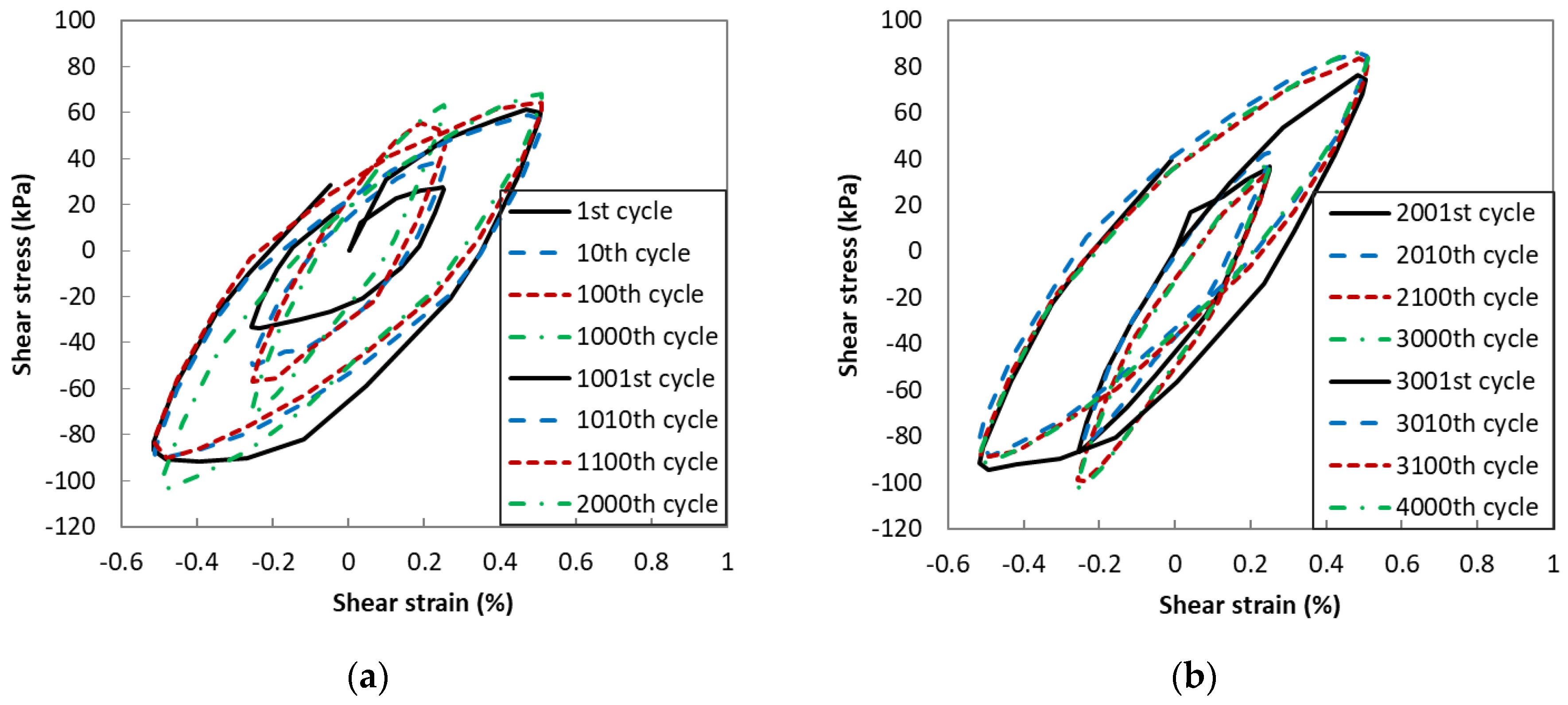
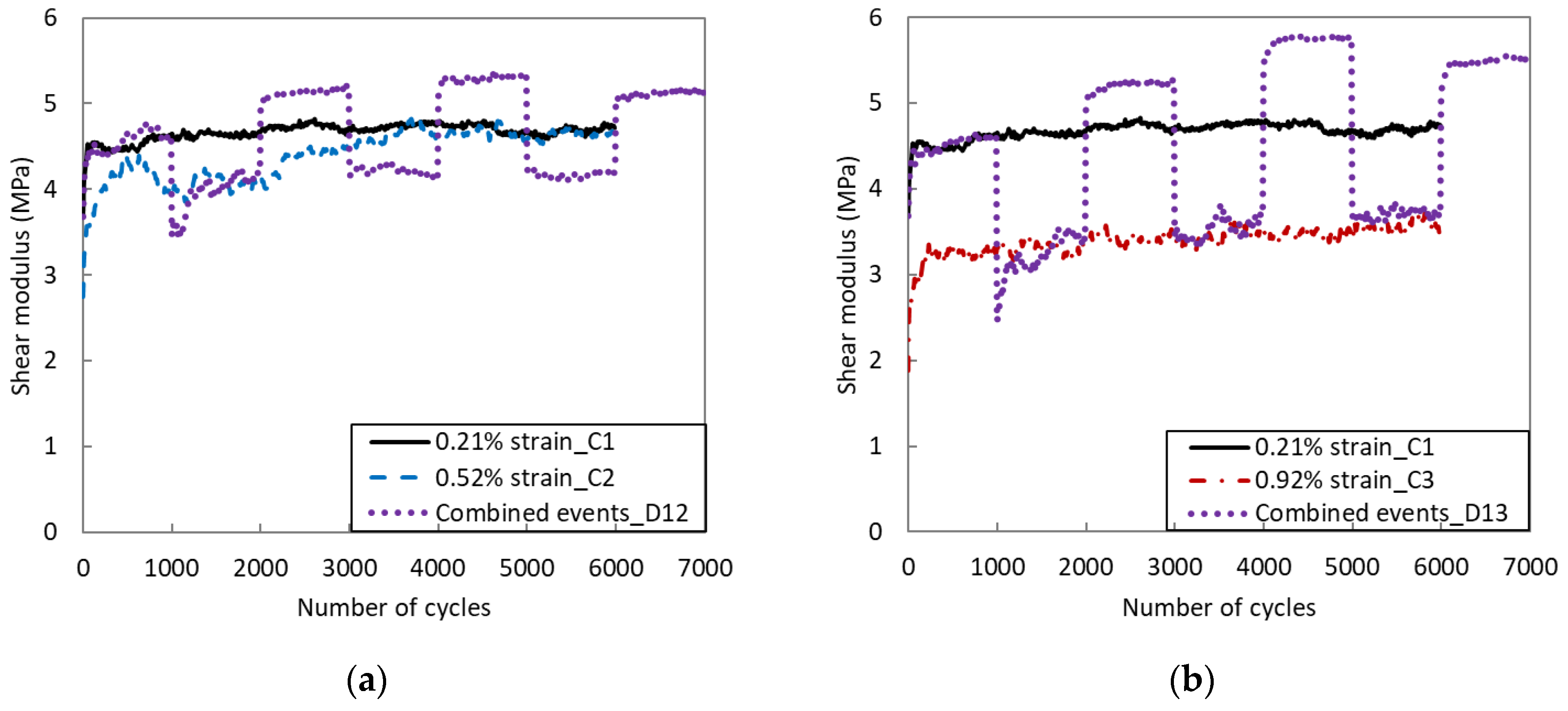
3.2.1. Stress–Strain Relationships
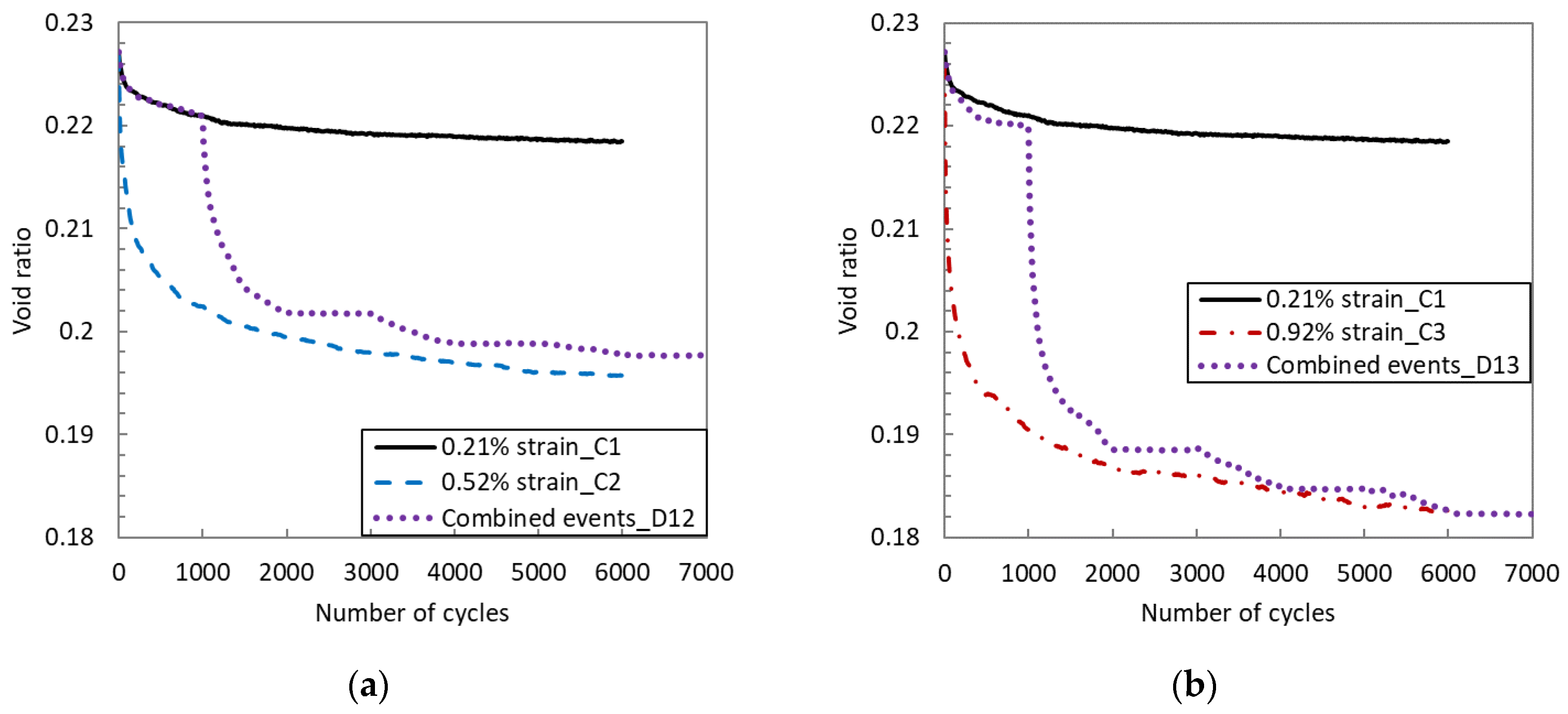
The representative cycles in the DEM simulation C2 with single strain amplitude of 0.52% are shown in Figure 9. Similar to the experimental tests, the maximum shear stress at γmax increases and the minimum shear stress at γmin decreases with an increasing number of cycles, leading to an increase in shear modulus and decrease in damping ratio. One difference between the experiments and DEM simulations is that the shape of the initial part of the stress–strain curve in DEM is concave upwards rather than concave downwards as in the experiments, i.e., the small strain stiffness first increases up to 0.2% and then decreases. The other difference is that once the strain reaches the maximum value and changes shearing direction, there is a delay in the reduction in stress: the stress first increases slightly then starts to decrease, thus forming a small loop at both ends of the hysteresis loop. These delays in stress reduction indicate the inertia effect of the particles in DEM, because the shear strain rate is a constant with sudden direction inversions in virtual simulations rather than the sinuous strain rate with smooth direction inversions in experiments.
The representative cycles in the combined weather events D12 are shown in Figure 10. Obviously, the areas of hysteresis loops for HSA events are much larger than those for LSA events. In the first LSA event (cycles 1–1000), an increase in shear modulus and a decrease in damping ratio are very clear. In the first HSA event (cycles 1001–2000), an increase in shear modulus and a decrease in damping ratio are also obvious, as the strain amplitude in this event is much higher than in the previous event. However, from Event 3 (cycles 2001–3000) onwards, no matter the strain amplitude, both shear modulus and hysteresis loop area only vary slightly. The DEM simulations show less variations than experimental tests. Possible reasons for this difference include the wider particle size distribution, particle breakage and interlocking between irregular shaped particles in physical samples, which enable more capacity for continuous variations and slower stabilisation.
The variation of the shear modulus with the number of loading cycles for both single weather conditions and combined weather conditions are illustrated in Figure 11. As expected, shear modulus (G) reduces with increasing strain amplitude (γ), agreeing with the typical Gγ degradation curve [34]. It is very clear that the shear modulus increases quickly in the first 1000 cycles and is stabilised afterwards in single weather conditions. The shear modulus for 0.21% (C1) and 0.52% (C2) approaches after 4000 cycles. In the combined weather events D12 and D13, Event 1 is consistent with the single strain amplitude of 0.21% (C1), while in Event 2 with γmax = 0.52% (or 0.92%), the shear modulus reduced to 3.5 MPa (or 2.5 MPa) in the first cycle, which is much higher than the initial shear modulus 2.8 MPa (or 1.9 MPa) for the single strain amplitude in C2 (C3). This is due to soil compaction during Event 1. At the end of Event 2, the shear modulus approaches the value for the 2000th cycle for the single strain amplitude, i.e., 4.1 MPa for 0.52% and 3.3 MPa for 0.92%. The difference starts from Event 3. In Event 3, all strain amplitudes are 0.21%, but both combined events have much higher shear moduli (5.2 MPa) than the single weather event (4.7 MPa) in the 3000th cycle. In Event 4, the shear modulus for D13 is similar to the modulus for C3; however, the shear modulus for D12 (4.2 MPa) is much lower than C2 (4.6 MPa). In Event 5 (γmax = 0.21%), the differences in the shear modulus for C1 and D12/D13 are more pronounced, i.e., 4.7 MPa and 5.3 MPa/5.7 MPa, respectively. The two consequent events replicated the observations in Event 4 and Event 5.

3.2.2. Void Ratio

To understand the variations of the shear moduli, the average void ratios of the samples were determined and are illustrated in Figure 12. It is clearly shown that the void ratio reduces under cyclic loading, and the higher the strain amplitude, the more the reduction in void ratio. Comparing Figure 12 and Figure 11, it can be found that the void ratio is another controlling parameter for the shear modulus for a single weather condition. The similarity of the shear moduli for C1 and C2 is due to the combined effect of strain amplitude and void ratio. In the combined weather conditions (D12 and D13), the void ratios for Events 3, 5 and 7 with γmax = 0.21% are much lower than that for C1, indicating denser soil conditions; thus the shear moduli are higher than that for C1. This also confirms the hypothesis made for these experiments. The void ratios for Events 2, 4 and 6 for D12 are always higher (soil is looser) than that for C2, therefore the shear modulus for D12 is lower.

3.2.3. Coordination Number

Another microscale parameter, the coordination number, which is the average contacts per particle, for all simulations are also plotted in Figure 13. The coordination number has a strong relation with the stress level within the sample [29]. First, the coordination number increases with cyclic loading. The coordination number for C1 is much lower than the other simulations. The coordination number is shown to be the third controlling parameter for shear moduli, as more contacts enable more transmissions of contact forces between particles, thus increasing the average stresses and stiffness. As the coordination number for C2 is much higher than that for C1, it is not surprising that its shear modulus rises to a greater extent. The coordination numbers for D12 and D13 also give an explanation to the observations of shear moduli: in Events 3, 5 and 7 where γmax = 0.21%, the coordination numbers for D12 and D13 are obviously higher than that for C1, leading to a higher shear modulus; in Events 2, 4 and 6, the coordination number for D12 is slightly lower than that for C2, leading to a lower shear modulus; D13 and C3 have similar coordination numbers and similar void ratios in Events 4 and 6, and thus similar shear moduli.

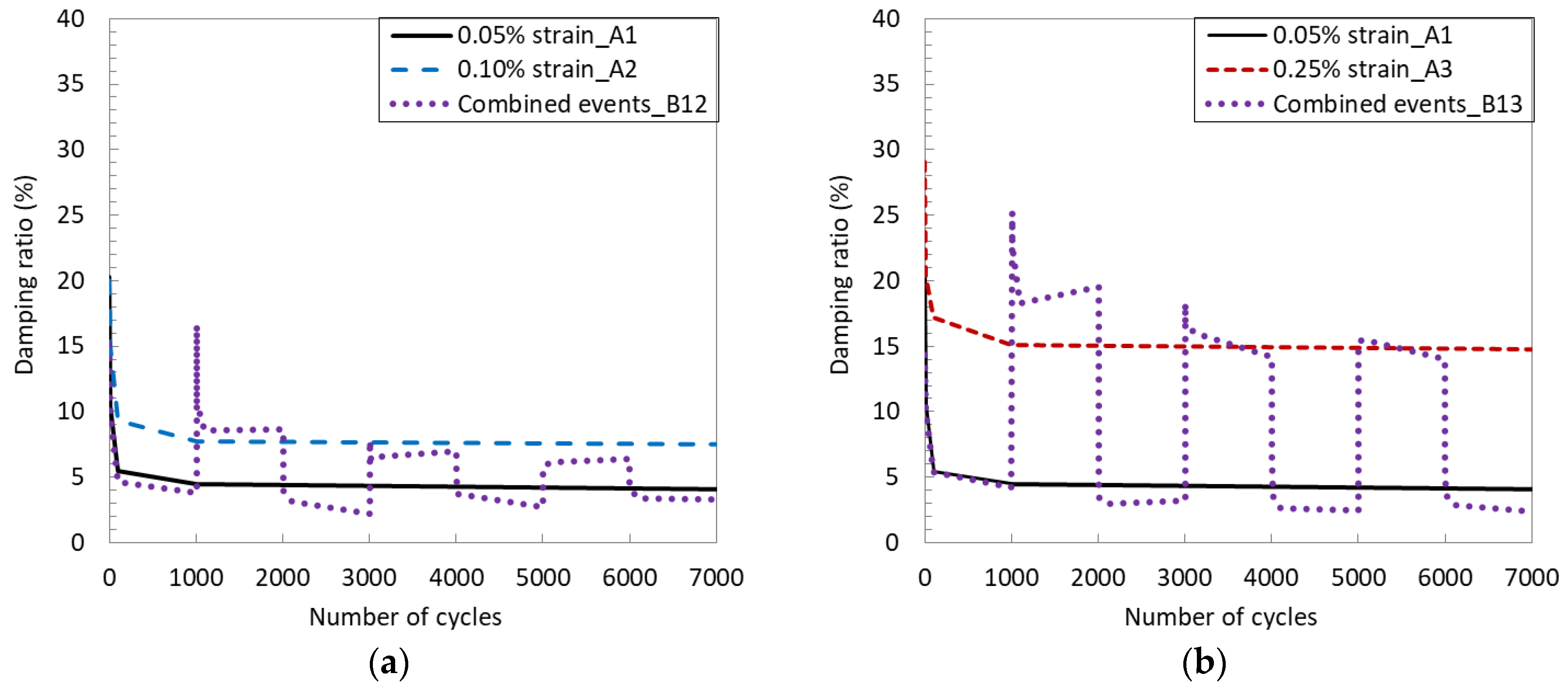
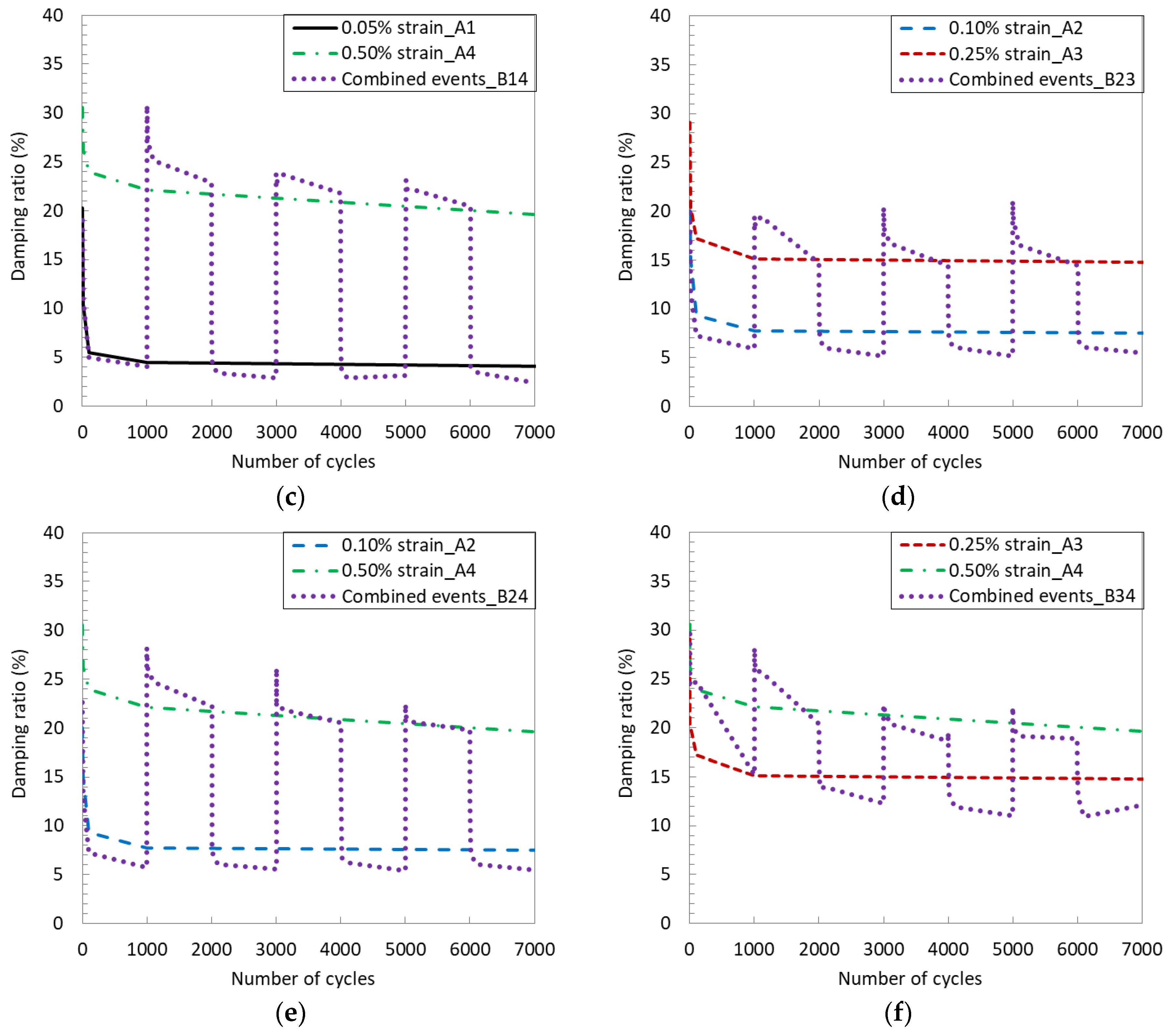
3.2.4. Damping Ratio

The variations in damping ratio for both a single weather condition and combined weather conditions are illustrated in Figure 14. For a single weather condition, the damping ratio drops significantly in the first few cycles and then mobilises at a steady value. For the combined weather conditions, damping ratios in Events 1, 3, 5 and 7 for D12 match the values for C1 with the same strain amplitude, while the damping ratio for D13 is similar to C1 in Events 1 and 3, but lower in Events 5 and 7. For Events 2, 4 and 6, the damping ratio for D12 (D13) matches the value for C2 (C3) in most cycles; however, in the first few cycles in Event 2, the damping ratio for D12 (D13) experiences a sharp increase, indicating a big disturbance in the soil sample and lots of soil rearrangements due to a sudden strain amplitude switch. Such sharp increases are not observed in Events 4 and 6, showing that soil tends to adapt to the strain amplitude switch and becomes stabilised. By comparing Figure 14 and Figure 8, it is observed that the magnitudes of damping ratios in DEM simulations are much lower than those in experimental tests. This is due to a number of factors: the DEM sample has a narrower particle size distribution and rounded particle shape, thus less capacity for smaller particles moving into voids or interlocking with each other and dissipating energy; real sand particles may break under cyclic loading and thus dissipate energy, but DEM particles are not breakable in current simulations. Nevertheless, DEM simulations successfully captured the key characteristics of dynamic parameter evolutions.

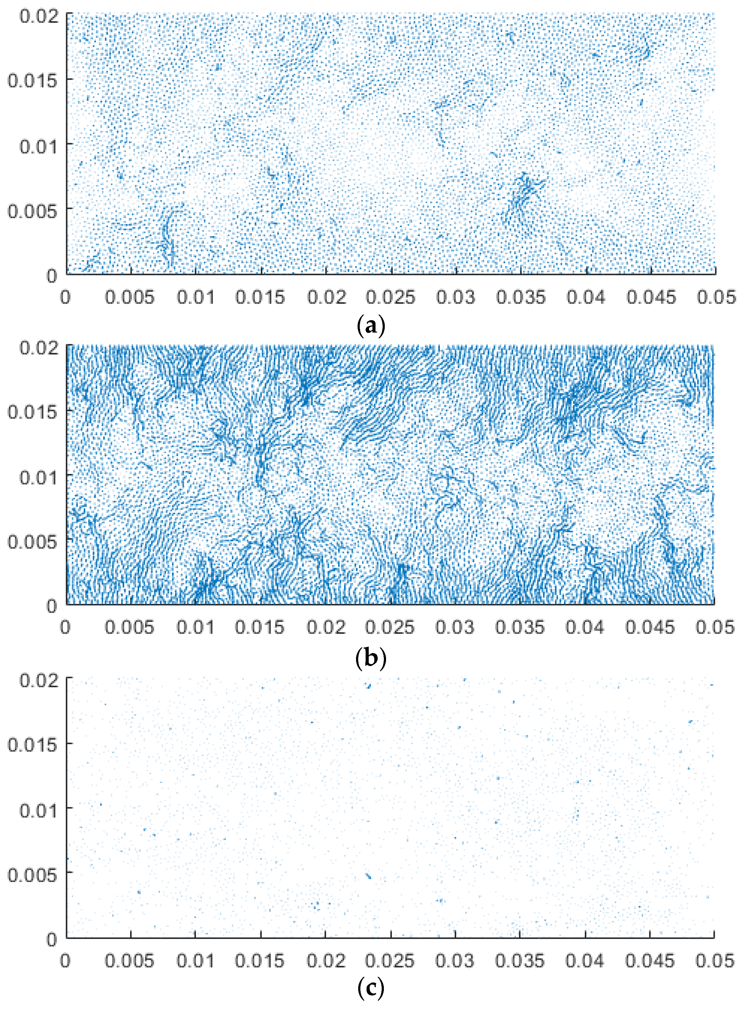
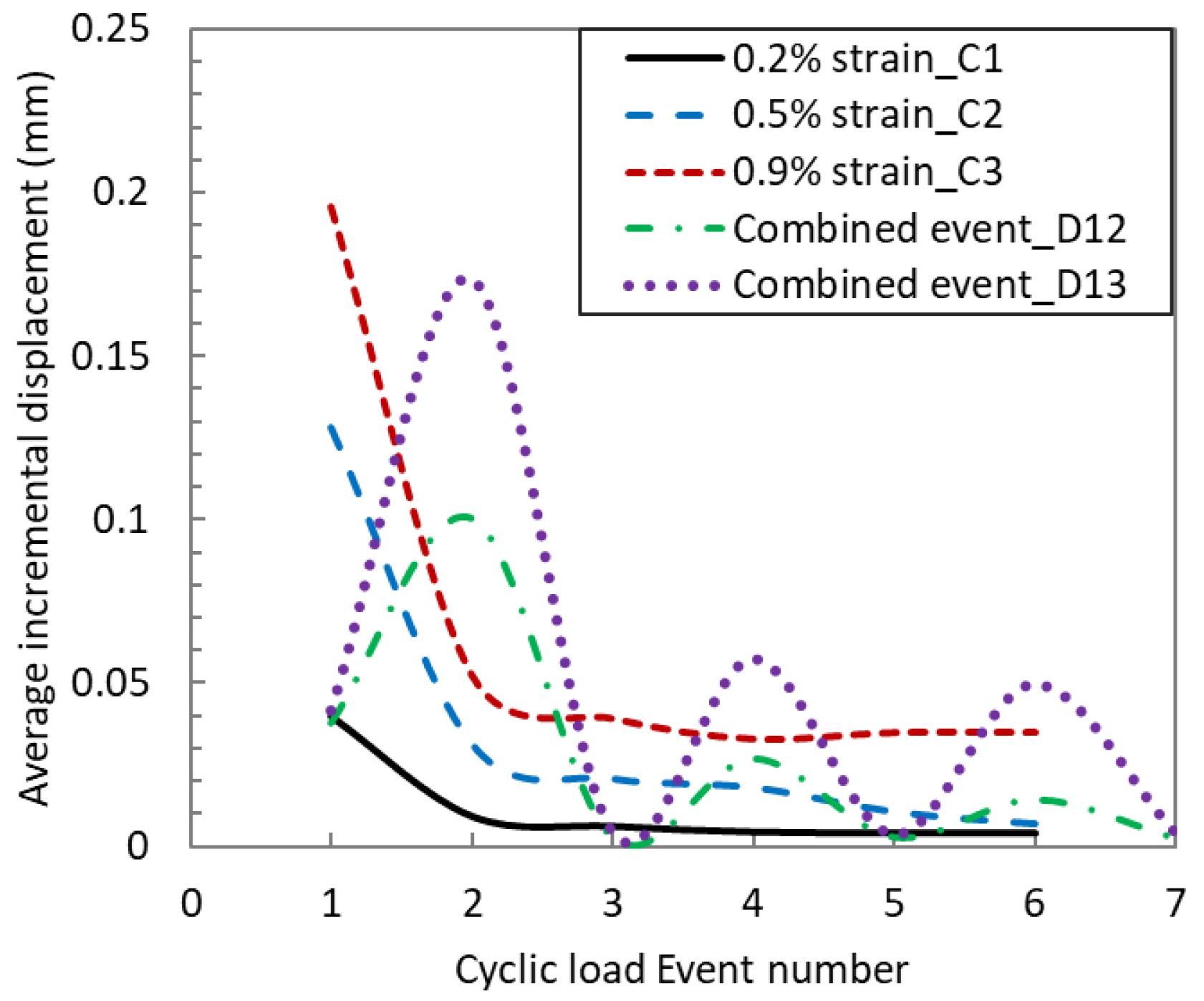
3.2.5. Incremental Particle Displacement

To confirm the hypothesis for the damping ratio, incremental particle displacement fields for C2 (γmax = 0.52%) and D12 (γmax = 0.21% + 0.52%) are illustrated in Figure 15 and Figure 16, respectively. In the plots, each vector starts from the initial location of a particle, pointing to the new location in each considered interval. Each vector is scaled by a factor of 3.0 to increase the visibility. It is clearly shown in Figure 15a that, in the first 1000 cycles, particles along the top and bottom boundaries mainly move inwards, leading to soil densification, consistent with the observations in the evolution of the void ratio. In the middle of the sample, there are lots of local convective flows forming granular vortices. Soil densification and soil convections are both associated with energy dissipation. In the second 1000 cycles, no clear soil densification can be observed, but local convective flows are still noticeable in the middle of the sample. In the third 1000 cycles, particle movements are very small. For the combined weather condition simulation D12, the first 1000 cycles are under 0.21% strain amplitude, thus the particle displacements are much smaller than those for 0.52%. In the second 1000 cycles, strain amplitude increased to 0.52%; consequently, the particle displacements increase significantly, including soil densification and convective flow. In the third 1000 cycles, strain amplitude is reduced to 0.21% again and very few noticeable particle displacements occur. In the fourth 1000 cycles, only convective flows can be observed under 0.52% strain amplitude.

4. Discussion and Conclusions

A summary of the average particle displacements for every 1000 cycles for all DEM simulations is shown in Figure 17. The average displacement reduces quickly with loading cycles for single weather conditions. For the combined events, the decay of particle displacement slows down, as every time the strain amplitude is increased, soil experiences extra excitation and has more rearrangements than that without the sandwich of low strain amplitude loading cycles. This reveals that soil can easily reach a dynamically stable state under regular cyclic loading, but with irregular cyclic loading, the excitation can drive the particle rearrangements and evolutions of dynamic properties further. A combination of two strain amplitudes has led to a bigger change; one can believe that if soil is excited by a real irregular dynamic loading signal, dynamic soil properties can experience further changes.
Although the DEM is limited to 2D simulations, i.e., a central slice of the cylindrical specimen, the observed variation trends for the shear modulus and damping ratio agree well with the experimental results. The percentage of increase in shear modulus is lower in DEM simulations and the damping ratio is also lower in DEM simulations. DEM samples tend to stablise quicker than physical samples. The main reasons are the narrower particle distribution and non-breakable particles. With wider particle distribution in experiments, fine particles can move into voids between coarse particles. In addition, with particle breakage under cyclic loading, more fine particles can be generated, and more energy dissipated, thus the particle rearrangements and increase in stiffness continue after more loading cycles.
In the current paper, both experimental tests and DEM modelling of cyclic simple shear tests were conducted to investigate the soil responses for soil–monopile interactions under varying weather conditions. Cyclic simple shear tests with combined strain amplitudes were considered to mimic the switches between normal weather conditions and extreme weather conditions. Based on the investigations, the following conclusions can be drawn:
  • The shear modulus of soil for loose sand increases quickly with cyclic loading initially and then mobilises around a steady value. The higher the strain amplitude, the lower the shear modulus, but the higher the increase.
  • The increase in the shear modulus is a combined consequence of reduction in void ratio and increase in coordination number due to particle movements.
  • The damping ratio of soil decreases quickly with cyclic loading initially and then also mobilises around a constant value. The higher the strain amplitude, the higher the damping ratio.
  • Soil becomes stabilised after thousands of loading cycles with a single strain amplitude.
  • The switch of strain amplitude between a low value and a high value can break the dynamic stabilisation of the soil and give soil more excitations, which lead to further particle rearrangements and thus further variations in the shear modulus and damping ratio.
The current study has a few limitations:
  • Cyclic loading with single strain amplitude is an idealised situation for the offshore loading environment. The current load patterns switching between two strain amplitudes simulate very basic varying weather conditions. To understand the soil response and soil–structure interactions in real offshore environments, real load signals will be considered in future experiments and numerical simulations.
  • Dried soil samples were analysed in the current study to replicate a fully drained condition because wind and wave load frequencies are relatively low and sandy soil is mainly in drained conditions. Seismic conditions were not considered.
  • The numerical simulations modelled the sand as an assembly of 2D rounded unbreakable disks with narrower particle distribution, which will not replicate all physical sample responses. However, they have been verified to be able to capture the key responses qualitatively. The purpose of numerical modelling is not to replicate the physical tests but provide insight into the micromechanism and advance engineers’ understanding of soil behaviours under complex loading.
The variations of soil stiffness and damping of granular soils under irregular cyclic loading can be used to develop/improve soil constitutive models (including p–y curves) under long-term cyclic loading to be used in SSI modelling of offshore structures in future studies. Future studies will consider the soil responses under real environment load signals and seismic loads and their influences on SSI for offshore structures.

Author Contributions

Conceptualization, L.C. and S.B.; data curation, L.C. and S.; methodology, L.C. and S.B.; software, L.C.; formal analysis, L.C., M.A. and S.; investigation, L.C. and S.; writing—original draft preparation, L.C. and S.; writing—review and editing, L.C., M.A. and S.B.; supervision, L.C. and S.B. All authors have read and agreed to the published version of the manuscript.

Funding

This research received no external funding.

Institutional Review Board Statement

Not applicable.

Informed Consent Statement

Not applicable.

Data Availability Statement

The data that support the findings of this study are openly available in GitHub at: https://github.com/clsnow2002/CSSVaryingWeather (accessed on 20 May 2023).

Conflicts of Interest

The authors declare no conflict of interest.

References

  1. Shajarati, A.; Sørensen, K.W.; Nielsen, S.K.; Ibsen, L.B. Behaviour of cohesionless soils during cyclic loading. In DCE Technical Memorandum No. 14; Department of Civil Engineering, Aalborg University: Aalborg, Denmark, 2012. [Google Scholar]
  2. Anestis, S.; Veletsos, J.W.M. Dynamic behaviour of building-foundation systems. Earthq. Eng. Struct. Dyn. 1974, 3, 121–138. [Google Scholar]
  3. Amendola, C.; de Silva, F.; Vratsikidis, A.; Pitilakis, D.; Anastasiadis, A.; Silvestri, F. Foundation impedance functions from full-scale soil-structure interaction tests. Soil Dyn. Earthq. Eng. 2021, 141, 106523. [Google Scholar] [CrossRef]
  4. Mina, D.; Forcellini, D. Soil–Structure Interaction Assessment of the 23 November 1980 Irpinia-Basilicata Earthquake. Geosciences 2020, 10, 152. [Google Scholar] [CrossRef] [Green Version]
  5. Roberto Paolucci, M.S.; Tolga Yilmaz, M. Seismic behaviour of shallow foundations: Shaking table experiments vs numerical modelling. Earthq. Eng. Struct. Dyn. 2008, 37, 577–595. [Google Scholar] [CrossRef]
  6. Jacob David Rodríguez Bordón, J.J.A.; Maeso, O.; Bhattacharya, S. Simple approach for including foundation–soil–foundation interaction in the static stiffnesses of multi-element shallow foundations. Géotechnique 2021, 71, 686–699. [Google Scholar] [CrossRef]
  7. Cui, L.; Bhattacharya, S.; Nikitas, G.; Bhat, A. Macro- and micro-mechanics of granular soil in asymmetric cyclic loadings encountered by offshore wind turbine foundations. Granul. Matter 2019, 21, 73. [Google Scholar] [CrossRef] [Green Version]
  8. Cui, L.; Bhattacharya, S. Soil–monopile interactions for offshore wind turbines. Proc. ICE Eng. Comput. Mech. 2016, 169, 171–182. [Google Scholar] [CrossRef] [Green Version]
  9. Kuhn, M. Dynamics of Offshore Wind Energy Converters on Mono-Pile Foundation Experience from the Lely Offshore Wind Turbine; OWEN (Offshore Wind Energy Network) Workshop: Swindon, UK, 2000. [Google Scholar]
  10. Achmus, M.; Kuo, Y.-S.; Abdel-Rahman, K. Behavior of monopile foundations under cyclic lateral load. Comput. Geotech. 2009, 36, 725–735. [Google Scholar] [CrossRef]
  11. Nikitas, G.; Arany, L.; Aingaran, S.; Vimalan, J.; Bhattacharya, S. Predicting long term performance of Offshore Wind Turbines using Cyclic Simple Shear apparatus. Soil Dyn. Earthq. Eng. 2016, 92, 678–683. [Google Scholar] [CrossRef] [Green Version]
  12. O’Sullivan, C.; Cui, L.; O’Neil, S. Discrete element analysis of the response of granular materials during cyclic loading. Soils Found. 2008, 48, 511–530. [Google Scholar] [CrossRef] [Green Version]
  13. Jalbi, S.; Arany, L.; Salem, A.; Cui, L.; Bhattacharya, S. A method to predict the cyclic loading profiles (one-way or two-way) for monopile supported offshore wind turbines. Mar. Struct. 2019, 63, 65–83. [Google Scholar] [CrossRef] [Green Version]
  14. Arany, L.; Bhattacharya, S.; Macdonald, J.; Hogan, S.J. Simplified critical mudline bending moment spectra of offshore wind turbine support structures. Wind Energy 2015, 18, 2025–2258. [Google Scholar] [CrossRef] [Green Version]
  15. Ji, X.; Zou, L.; Yang, Z.; Wang, D.; Bingham, H.B. Numerical research on the interaction of multi-directional random waves with an offshore wind turbine foundation. Ocean. Eng. 2022, in press. [Google Scholar] [CrossRef]
  16. DNVGL-ST-0437; Loads and Site Conditions for Wind Turbines. DNV GL: Oslo, Norway, 2016.
  17. IEC-61400; Wind Energy Generation Systems-Part 12-1: Power Performance Measurements of Electricity Producing Wind Turbines. IEC: Geneva, Switzerland, 2017.
  18. Banerjee, A.; Chakraborty, T.; Matsagar, V.; Achmus, M. Dynamic analysis of an offshore wind turbine under random wind and wave excitation with soil-structure interaction and blade tower coupling. Soil Dyn. Earthq. Eng. 2019, 125, 105699. [Google Scholar] [CrossRef]
  19. Charlton, T.; Rouainia, M. Geotechnical fragility analysis of monopile foundations for offshore wind turbines in extreme storms. Renew. Energy 2022, 182, 1126–1140. [Google Scholar] [CrossRef]
  20. Li, W.; Igoe, D.; Gavin, K. Field tests to investigate the cyclic response of monopiles in sand. Proc. Inst. Civ. Eng. Geotech. Eng. 2014, 168, 407–421. [Google Scholar] [CrossRef]
  21. Lombardi, D.; Bhattacharya, S.; Wood, D.M. Dynamic soil–structure interaction of monopile supported wind turbines in cohesive soil. Soil Dyn. Earthq. Eng. 2013, 49, 165–180. [Google Scholar] [CrossRef]
  22. Cuéllar, P.; Georgi, S.; Baeßler, M.; Rücker, W. On the quasi-static granular convective flow and sand densification around pile foundations under cyclic lateral loading. Granul. Matter 2012, 14, 11–25. [Google Scholar] [CrossRef]
  23. Zhu, F.Y.; O’Loughlin, C.D.; Bienen, B.; Cassidy, M.J.; Morgan, N. The response of suction caissons to long-term lateral cyclic loading in single-layer and layered seabeds. Geotechnique 2018, 68, 729–741. [Google Scholar] [CrossRef]
  24. Li, Z.; Haigh, S.K.; Bolton, M.D. Centrifuge modelling of mono-pile under cyclic lateral loads. In Physical Modelling in Geotechnics, Two Volume Set, Proceedings of the 7th International Conference on Physical Modelling in Geotechnics (ICPMG 2010), Zurich, Switzerland, 28 June–1 July 2010; CRC Press: Leiden, The Netherlands, 2010; Volume 2, pp. 965–970. [Google Scholar]
  25. Duan, N.; Cheng, Y.; Xu, X. Distinct-element analysis of an offshore wind turbine monopile under cyclic lateral load. Proc. Inst. Civ. Eng. Geotech. Eng. 2017, 170, 517–533. [Google Scholar] [CrossRef] [Green Version]
  26. Zhu, N.; Cui, L.; Liu, J.; Wang, M.; Zhao, H.; Jia, N. Discrete element simulation on the behavior of open-ended pile under cyclic lateral loading. Soil Dyn. Earthq. Eng. 2021, 144, 106646. [Google Scholar] [CrossRef]
  27. Mendoza-Ulloa, J.A.; Lombardi, D.; Ahmad, S.M. Small-strain stiffness degradation of artificially cemented sands. Géotech. Lett. 2020, 10, 284–289. [Google Scholar] [CrossRef]
  28. D6528-07; Standard Test Method for Consolidated Undrained Direct Simple Shear Testing of Cohesive Soils. ASTM: West Conshohocken, PA, USA, 2007.
  29. O’Sullivan, C. Particulate Discrete Element Modelling: A Geomechanics Perspective; CRC Press: Boca Raton, FL, USA, 2017. [Google Scholar]
  30. Itasca. PFC2D User’s Manual 4.0; Itasca Consulting Group Inc.: Minneapolis, MN, USA, 2008. [Google Scholar]
  31. Cavarretta, I. The Influence of Particle Characteristics on the Engineering Behaviour of Granular Materials. Ph.D. Thesis, Imperial College, London, UK, 2009. [Google Scholar]
  32. DNV-OS-J101; Design of Offshore Wind Turbine Structures. DNV: Høvik, Norway, 2014.
  33. Karg, C. Modelling of Strain Accumulation due to Low Level Vibrations in Granular Soils; Ghent University: Ghent, Belgium, 2007. [Google Scholar]
  34. Atkinson, J.H. The Mechanics of Soils and Foundations, 2nd ed.; Taylor & Francis: Abingdon, UK, 2007. [Google Scholar]
Figure 1. Particle size distribution (PSD) of RedHill 110 sand in experiments and PSD of DEM samples.
Jmse 11 01222 g001
Figure 2. Schematic diagram of loading cycle patterns for varying weather conditions.
Jmse 11 01222 g002
Figure 3. Configuration of the soil sample generated using DEM and locations of measurement circles.
Jmse 11 01222 g003
Figure 4. Representative stress–strain loops for Test A4 with 0.5% strain amplitude with indicative triangles for calculations of damping ratio (Red arrows indicate increasing number of cycles).
Jmse 11 01222 g004
Figure 5. Representative stress–strain loops for Test B34. (a) Event 1 (LSA) and Event 2 (HSA). (b) Event 3 (LSA) and Event 4 (HSA).
Jmse 11 01222 g005
Figure 6. Evolution of dynamic parameters during cyclic loading for Series A. (a) Shear modulus. (b) Damping ratio.
Jmse 11 01222 g006
Figure 7. Comparison of shear moduli between a combined event and its corresponding single strain amplitude events for experiments. (a) A1, A2 and B12. (b) A1, A3 and B13. (c) A1, A4 and B14. (d) A2, A3 and B23. (e) A2, A4 and B24. (f) A3, A4 and B34.
Jmse 11 01222 g007aJmse 11 01222 g007b
Figure 8. Comparison of damping ratios between a combined event and its corresponding single strain amplitude events for experiments. (a) A1, A2 and B12. (b) A1, A3 and B13. (c) A1, A4 and B14. (d) A2, A3 and B23. (e) A2, A4 and B24. (f) A3, A4 and B34.
Jmse 11 01222 g008aJmse 11 01222 g008b
Figure 9. Representative stress–strain loops for Simulation C2 with 0.52% strain amplitude (Red arrows indicate increasing number of cycles).
Jmse 11 01222 g009
Figure 10. Representative stress–strain loops for Simulation D12. (a) Event 1 (LSA) and Event 2 (HSA). (b) Event 3 (LSA) and Event 4 (HAS).
Jmse 11 01222 g010
Figure 11. Comparison of shear moduli between a combined event and its corresponding single strain amplitude events for DEM simulations. (a) C1, C2 and D12. (b) C1, C3 and D13.
Jmse 11 01222 g011
Figure 12. Comparison of void ratios between a combined event and its corresponding single strain amplitude events for DEM simulations. (a) C1, C2 and D12. (b) C1, C3 and D13.
Jmse 11 01222 g012
Figure 13. Comparison of coordination numbers between a combined event and its corresponding single strain amplitude events for DEM simulations. (a) C1, C2 and D12. (b) C1, C3 and D13.
Jmse 11 01222 g013
Figure 14. Comparison of damping ratios between a combined event and its corresponding single strain amplitude events for DEM simulations. (a) C1, C2 and D12. (b) C1, C3 and D13.
Jmse 11 01222 g014
Figure 15. Incremental displacement field for C2 (Unit: m). (a) First 1000 cycles—0.52%. (b) Second 1000 cycles—0.52%. (c) Third 1000 cycles—0.52%.
Jmse 11 01222 g015aJmse 11 01222 g015b
Figure 16. Incremental displacement field for D12 (Unit: m). (a) First 1000 cycles—0.21%. (b) Second 1000 cycles—0.52%. (c) Third 1000 cycles—0.21%. (d) Fourth 1000 cycles—0.52%.
Jmse 11 01222 g016aJmse 11 01222 g016b
Figure 17. Average particle displacement in each event for all DEM simulations.
Jmse 11 01222 g017
Table 1. Experimental test and DEM simulation program.
Series NameTest No.Shear Strain %Cycles
Experimental testsAA10.0530,000
A20.130,000
A30.2530,000
A40.530,000
BB12 *0.05 + 0.11000/event
B130.05 + 0.251000/event
B140.05 + 0.51000/event
B230.1 + 0.251000/event
B240.1 + 0.51000/event
B340.25 + 0.51000/event
DEM simulationsCC10.216000
C20.526000
C30.926000
DD120.21 + 0.521000/event
D130.21 + 0.921000/event
* Index “12” in “B12” means B12 is a combination of A“1” and A“2”.
Table 2. DEM simulation parameters.
DEM ParameterValue
Particle density2650 kg/m3
Frictional coefficient0.5
Normal stiffness of particle8.0 × 107 N/m
Shear stiffness of particle4.0 × 107 N/m
Normal and shear stiffness of boundary4.0 × 109 N/m
Disclaimer/Publisher’s Note: The statements, opinions and data contained in all publications are solely those of the individual author(s) and contributor(s) and not of MDPI and/or the editor(s). MDPI and/or the editor(s) disclaim responsibility for any injury to people or property resulting from any ideas, methods, instructions or products referred to in the content.

