PIV Snapshot Clustering Reveals the Dual Deterministic and Chaotic Nature of Propeller Wakes at Macro- and Micro-Scales

Abstract

This study investigates the underlying mechanisms governing the evolution of tip vortices in the far field of a naval propeller wake. To achieve this, a novel approach utilizing data clustering applied to particle image velocimetry snapshots is employed. The clustering of data is carried out using the k-means algorithm, with the optimal number of clusters determined by evaluating two metrics: the within-cluster sum of squares and the average silhouette. The clustering of phase-locked propeller wake data is focused on the vorticity associated with the regions containing tip vortices. Additionally, techniques such as proper orthogonal decomposition, t-distributed stochastic neighbor embedding, and kernel density estimation are employed to visually represent the data clusters in a two-dimensional space, facilitating their assessment and subsequent discussion. This paper shows how the application of data clustering enables a comprehensive understanding of the complex mechanisms driving the dynamics of propeller wake vortices in both the transitional and far fields. Specifically, it reveals the dual nature of the propeller wake flow, characterized by deterministic and chaotic behavior at macro- and micro-scales.

1. Introduction

The knowledge of the underlying mechanisms of propeller/rotor tip vortex evolution in the far field is an intriguing and still open problem of fluid dynamic research, which plays an important role in many applications of marine, aerospace, and mechanical engineering because of its impact on performance, vibrations, noise, and structural problems. A prominent example is wind parks, where power production, radiated sound, and fatigue lifetime of interior turbines might be significantly affected by the dynamics of the wake vortices released from surrounding turbines, see, e.g., [1,2,3]. Previous studies [4,5] have shown that propeller wake instability is driven by mutual inductance mechanisms, which lead adjacent vortex filaments to pair analogously to the leapfrogging motion of two inviscid vortex rings [6,7]. 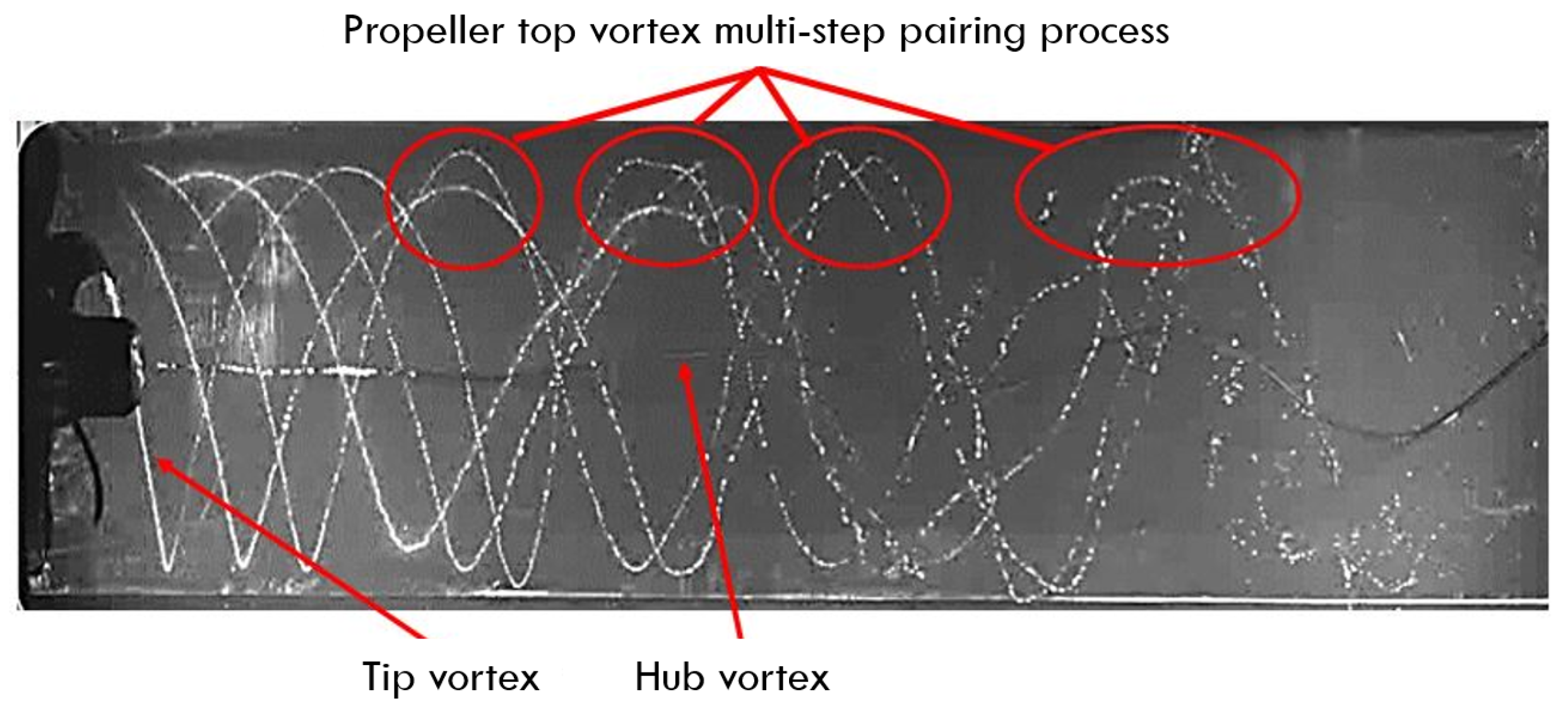Vortex pairing [4,8,9] manifests through a multi-step grouping process that depends on the blade number. This behavior has been highlighted by flow visualizations and phase-locked particle image velocimetry (PIV) measurements in the propeller transitional and far fields [10,11]. In spite of these results and to the authors’ best knowledge, rigorous, in-depth analyses focused on classifying the nature of the propeller tip vortex dynamics in the far field are still extremely limited, likely due to the complexity associated with the inherently multi-scale, highly turbulent, strongly unsteady nature of the flow, which makes its survey extremely challenging even using the most advanced experimental and computational tools.

Data science, machine learning, and artificial intelligence have emerged as cutting-edge research fields where rigorous methods and algorithms are developed and applied to gain knowledge from data. In recent years, these methods have been applied in the context of more traditional disciplines to accelerate the experimental/computational analysis process and extract insights from experiments and simulation data. In the field of ship hydrodynamics, supervised machine learning techniques, such as surrogate modeling, regression, and multi-fidelity methods, have been employed to integrate experimental and simulation data. These methods aim to reduce the computational burden associated with design performance assessment and optimization procedures along with facilitating the interpretation of the physics observed. Furthermore, unsupervised machine learning methods, including equivalent approaches to proper orthogonal decomposition (POD) and/or linear/non-linear principal component analysis (PCA), have been utilized to address challenges such as dimensionality reduction, efficient design, and operational space exploration, and gain insights into complex physical phenomena. POD, which is closely related to PCA, has found widespread application in the identification of coherent structures within turbulent flows [12] and has been employed in the study of various flow configurations, including steady and transient jets [13,14] and marine propeller wakes [5]. By decomposing the flow into a linear combination of orthogonal eigenfunctions, POD provides valuable information about the spatial and temporal structure of the flow, enabling the construction of reduced-order models. However, it is important to note that while POD enjoys established global optimality properties, its effectiveness may be limited when investigating non-linear, transient, non-stationary, and non-ergodic dynamics. To address these limitations, non-linear dimensionality reduction (NLDR) methods have been developed and applied to gain a deeper understanding of data structures and physical phenomena. One straightforward approach to NLDR in conjunction with POD/PCA is to employ data clustering methods and perform POD/PCA within each cluster. This approach allows for a more comprehensive analysis and characterization of the underlying dynamics.

Cluster-based reduced-order modeling through POD/PCA offers valuable insights into complex phenomena by employing local PCA (LPCA), which partitions the dataset into clusters and applies POD/PCA within each cluster, assuming an approximate linear structure within them. The cluster centroids, together with their associated modes, capture relevant flow features in the spatial and temporal domains. Previous studies have demonstrated the application of spatial clustering using the k-means method with POD/PCA for analyzing a transient buoyant jet [15] and for characterizing a swirl-stabilized combustor flow through temporal and spatial k-means clustering [16]. It is worth noting that the choice of the number of clusters and the similarity metrics used for data clustering significantly impact the quality of the resulting reduced-order/dimensionality model, thereby influencing the extraction of meaningful physical insights from the clustering analysis. Rigorous data-clustering methods have been proposed in various fields to facilitate a deeper understanding of experimental and simulation data. To achieve fully non-linear dimensionality reduction, a promising technique called t-distributed stochastic neighbor embedding (t-SNE) has been proposed [17]. This method allows for embedding and visualizing high-dimensional data in a low-dimensional space and has been successfully applied to turbulence datasets from simulations [18].

Examples of data-clustering analysis applied to PIV experimental data are still limited, see, e.g., [19], where k-means is applied to study the internal aerodynamics of a Miller cycle gasoline engine. Examples of data-clustering analyses applied to propeller performance and, in general, vortex dynamics are also limited. Calvet et al. [20] developed an unsupervised machine learning strategy to automatically cluster vortex wakes of bio-inspired propulsors into groups of similar propulsive thrust and efficiency metrics. Doijode et al. [21] introduced a clustering approach for optimizing propellers by directing the search for the optimal design towards design clusters with good performance, i.e., high propulsive efficiency and low cavitation. Finally, Sharma and Simula [22] considered computer-generated configurations of quantized vortices in planar superfluid Bose–Einstein condensates, showing how data-clustering approaches can be successfully used for classifying vortex configurations to identify prominent vortex phases of matter.

The objective of this study is to establish a systematic approach for conducting a data-clustering analysis of PIV data to gain valuable physical insights into the dynamics of propeller tip vortices. Phase-locked PIV snapshots recorded throughout the transitional and far fields of a propeller wake (see Figure 1) are used in the clustering analysis.

Specifically, the velocity fields under investigation are obtained from experimental tests with large-scale, phase-locked, PIV measurements. Data were collected in the cavitation tunnel of CNR-INM [23]. The clustering of PIV data is based on the k-means algorithm. Data clustering is applied to phase-locked snapshots to gain knowledge on the topology of wake instability and its stochastic realizations. The vorticity is used as a clustering variable. 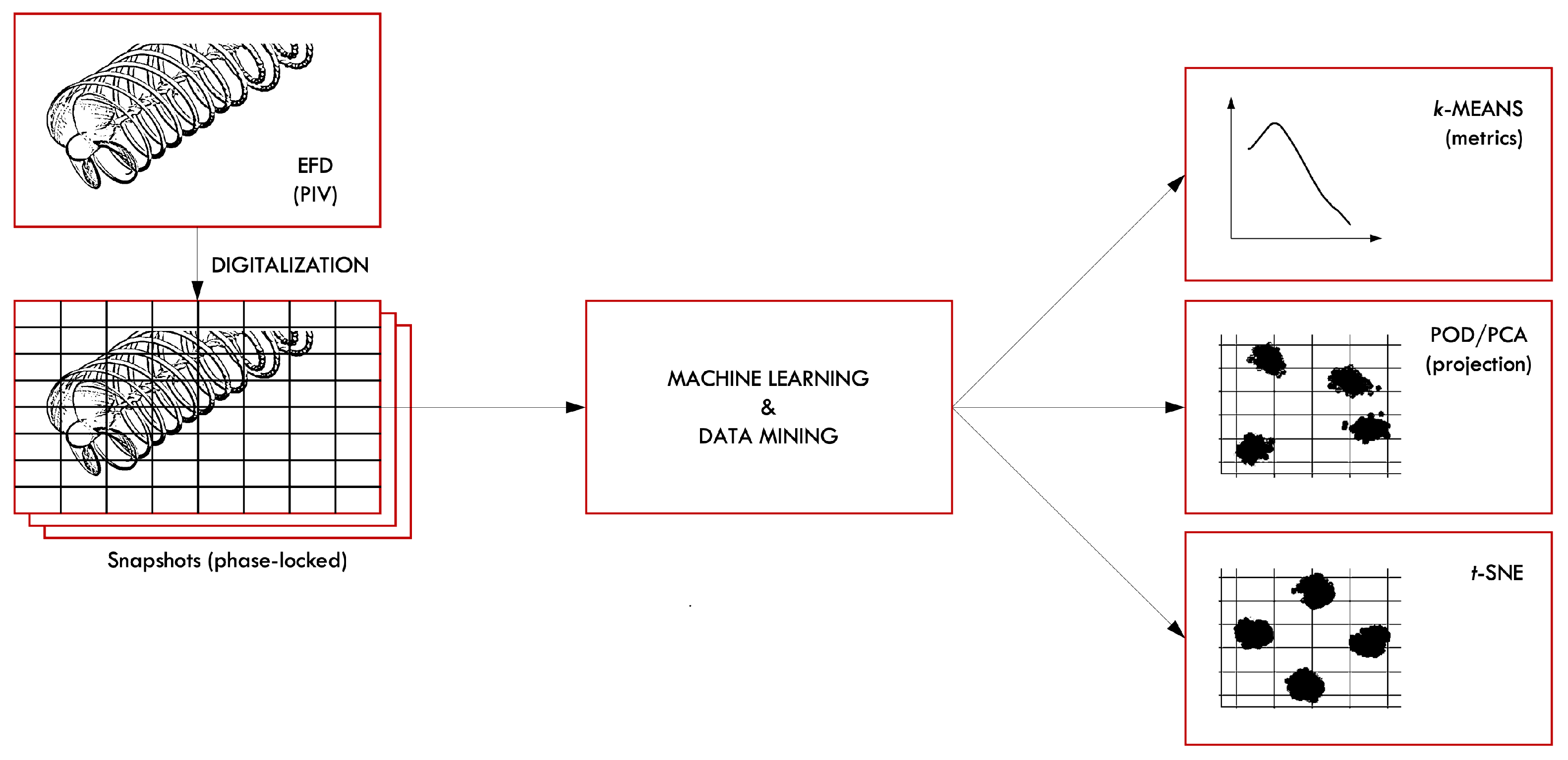The resulting cluster centroids identify the topology of the instability, where two or more tip vortices interact and coalesce [4,11]. Two metrics are used for the identification and assessment of clustering methods, including the selection of the proper number of clusters, namely: (i) within-cluster sum of squares and (ii) average silhouette. Additionally, the embedding of data via POD/PCA and t-SNE is used to define and visualize data clusters in a reduced dimensionality space. Finally, kernel density estimation (KDE) is applied to POD/PCA and t-SNE representations to provide continuous data distributions for assessment and discussion. The overall workflow is synthesized in Figure 2.

The remainder of the paper is organized as follows: experimental details are provided in Section 2; Section 3 presents the data analysis methods and metrics; the numerical results are presented in Section 4; finally, conclusions and future perspectives are given in Section 5.

2. Experimental Methods

The present study is based on a comprehensive database of flow measurements of the E1658 submarine propeller wake in open water using 2D-PIV [5,24], see Figure 1. The database covers an extensive set of propeller conditions in terms of advance coefficients and blade number configurations, providing a wide range of vortex instability and interaction mechanisms that are crucial for the objectives of the present study. In particular, the present study focuses on a propeller configuration with four blades and one value of the advance ratio, corresponding to a high propeller loading (i.e., $J=0.56$).

The experimental campaign was carried out at the CNR-INM cavitation tunnel, measuring the propeller wake flow at the vertical center-plane by a 2D-PIV system. The setup consisted of three 5 Mpx sCMOS cameras by PCO and two 200 mJ Nd-Yag Lasers by QUANTEL. Either cameras and lasers were positioned side by side to simultaneously record/illuminate a long portion of the wake flow (i.e., from the propeller plane to 3.3 D downstream, where D is the propeller diameter) at full resolution (4, 22, 23). This arrangement (see Figure 3), already adopted in other similar experiments [5,10,11], allowed the simultaneous reconstruction of a long portion of the wake flow (i.e., from the propeller plane to 3.3 D downstream, where D is the propeller diameter) without jeopardizing the spatial resolution.

The camera acquisition process was synchronized with the propeller reference blade at a specific angular position, facilitated by the coordination of four cameras and two lasers with a TTL OPR (Once Per Revolution) signal. This signal was generated by a rotary incremental encoder mounted on the propeller dynamometer, providing a frequency of 3600 pulses per second.

Hollow glass spheres, featuring a nominal diameter of 10 μm and a specific weight of 1.05 g/cm³, were utilized as tracers in the experiment. The acquired images underwent pre-processing using a local background subtraction routine with a 4 × 4 px² kernel. This pre-processing step effectively eliminated unwanted reflections and improved the signal-to-noise ratio. The vector calculation was performed using the advanced iterative multi-pass, multi-grid, image deformation algorithm [25]. Leveraging the GPU architecture of the workstation and the PIV algorithm, a combination of direct cross-correlation and parallel processing was employed, enabling both accurate and efficient evaluation of the images. The interrogation windows were iteratively reduced to a final size of 32 × 32 px², with a 50% overlap between adjacent windows.

3. Numerical Methods

The subsequent section presents an overview of the data analysis methods and metrics employed in this study. Specifically, we briefly describe and discuss the k-means clustering and t-SNE methods as visualization techniques, along with KDE. Additionally, two metrics, namely the within-cluster sum of squares and the average silhouette, are utilized to assess the clustering approaches and determine the optimal number of clusters, denoted as k.

3.1. k-Means Clustering

The k-means clustering method [26] is commonly used to build partitions of data, represented by an $[L\times S]$ matrix $\mathbf{D}$ (see below Equation (2)), into k distinct sets or clusters. Each cluster is defined by a representative point known as a centroid. The rearrangement of the original data in $\mathbf{D}$ is performed according to the specific clustering approach and criterion utilized. Generally, we denote each realization or point of the rearranged data as ${\mathbf{d}}_j$. Note that, generally, ${\mathbf{d}}_j\in {\mathbb{R}}^Q$ with $j=1,\dots ,H$, where $Q\ne L$ and $H\ne S$.

To measure the similarity between data points ${\mathbf{d}}_j$ and evaluate the cluster centroids ${\mathit{\mu }}_i$, the Euclidean distance is utilized. The centroids ${\mathit{\mu }}_i$ are obtained by averaging all data points within the i-th cluster ${\mathbf{K}}_i$. The assignment of data points to the k clusters is accomplished by minimizing the squared Euclidean distance between ${\mathbf{d}}_j$ and ${\mathit{\mu }}_i$, known as the within-cluster sum of squares (WCSS):

$$\mathrm{WCSS}=\sum _{i=1}^k\sum _{{\mathbf{d}}_j\in {\mathbf{K}}_i}{\parallel {\mathbf{d}}_j-{\mathit{\mu }}_i\parallel }^2$$

(1)

Solving the minimization problem in Equation (1) is known to be NP-hard [27]. To tackle this challenge, the heuristic approach proposed in [28] is employed. It is worth noting that the results obtained are highly sensitive to the initialization of the centroids. In this study, the initialization strategy suggested in [29] is utilized.

3.2. Proper Orthogonal Decomposition/Principal Component Analysis

The implementation of POD/PCA is carried out as follows. The data matrix $\mathbf{D}$ with dimensions $[L\times S]$ is defined as

$$\mathbf{D}=\left[\begin{array}{ccc}{\mathbf{d}}^{\left(1\right)}|& \dots & |{\mathbf{d}}^{\left(S\right)}\end{array}\right]$$

(2)

where $\mathbf{d}={\{d_1\left({\mathbf{x}}_1\right),\dots ,d_1\left({\mathbf{x}}_P\right),\dots ,d_M\left({\mathbf{x}}_1\right),\dots ,d_M\left({\mathbf{x}}_P\right)\}}^{\mathsf{T}}$ represents the collection of M discretized components of the quantity of interest $\mathbf{d}$. Each vector ${\mathbf{d}}^{\left(s\right)}$ corresponds to a snapshot at time realization s, while ${\mathbf{x}}_i$ denotes the i-th node of the spatial discretization. The size of the spatial discretization is denoted by P, resulting in $L=MP$.

The dimensionality of the data matrix $\mathbf{D}$ is reduced by projecting the snapshots onto a new linear subspace formed by the eigenvectors of the covariance matrix $\mathbf{C}$ of dimensions $[L\times L]$ [30]:

$$\mathbf{C}=\frac{1}{S}\mathbf{D}{\mathbf{D}}^{\mathsf{T}}$$

(3)

The eigenvectors (${\mathbf{z}}_i$) and eigenvalues (${\lambda }_i$) of $\mathbf{C}$ are obtained by solving the eigenvalue problem:

$$\mathbf{C}\mathbf{Z}=\mathbf{Z}\mathbf{\Lambda }$$

(4)

Alternatively, the problem in Equation (4) can be solved using the singular value decomposition (SVD) [31]. In cases where $L>S$, the dual problem can be solved using the snapshot-POD formulation [32].

The eigenvalues obtained from POD/PCA represent the variance explained by the corresponding eigenvectors. The linear subspace formed by the N eigenvectors (POD/PCA modes, collected in $\widehat{\mathbf{Z}}$) associated with the largest N eigenvalues captures the highest amount of variance/energy compared to other linear subspaces of dimension N [30,33]. The cumulative sum of the eigenvalues is used to assess the variance resolved by the linear subspace of dimension N.

Finally, the reconstructed data matrix $\widehat{\mathbf{D}}$ is given by:

$$\widehat{\mathbf{D}}=\widehat{\mathbf{Z}}{\widehat{\mathbf{Z}}}^{\mathsf{T}}\mathbf{D}$$

(5)

In this equation, the coefficient ${\mathit{\alpha }}_i={\widehat{\mathbf{z}}}_i^{\mathsf{T}}\mathbf{D}$ represents the projection of the data matrix onto the i-th mode.

3.3. t-Distributed Stochastic Neighbor Embedding

The t-SNE is a machine learning algorithm proposed by [17], which is found very effective for embedding high-dimensional data for visualization in a low-dimensional space of two or three dimensions. The t-SNE first constructs joint probability densities $p_{ij}$ that reflect pairwise similarity among data-points ${\mathbf{d}}^{\left(i\right)}$ and ${\mathbf{d}}^{\left(j\right)}$ parameterized by a Gaussian distribution

$$p_{ij}=\frac{p_{j|i}+p_{i|j}}{2S}$$

(6)

with

$$p_{j|i}=\frac{exp(-||{\mathbf{d}}^{\left(i\right)}-{\mathbf{d}}^{\left(j\right)}|{|}^2/2{\varsigma }_i^2)}{{\sum }_{k\ne i}^{S}exp(-||{\mathbf{d}}^{\left(i\right)}-{\mathbf{d}}^{\left(k\right)}|{|}^2/2{\varsigma }_i^2)}$$

(7)

In a similar manner, the joint probability densities $q_{ij}$ are defined for the low-dimensional representations ${\mathit{\alpha }}_i$ and ${\mathit{\alpha }}_j$, parameterized by a t-student distribution

$$q_{ij}=\frac{(1+||{\mathit{\alpha }}_i-{\mathit{\alpha }}_j{\left|\right|}^2{)}^{-1}}{{\sum }_{k\ne i}^S(1+||{\mathit{\alpha }}_i-{\mathit{\alpha }}_k{\left|\right|}^2{)}^{-1}}$$

(8)

The points (or coefficients) ${\mathit{\alpha }}_i$ are determined by minimizing the Kullback–Leibler divergence of the distribution Q from the distribution P as

$$\mathrm{KL}\left(P\right|\left|Q\right)=\sum _{i\ne j}^S{p}_{ij}log\left(\frac{p_{ij}}{q_{ij}}\right)$$

(9)

The minimization of Equation (9) with respect to the points ${\alpha }_i$ is performed using gradient descent. The parameter ${\varsigma }_i$ is set in such that the perplexity of the conditional distribution $P_i={\sum }_j{p}_{ji}$ over all data points given ${\mathbf{d}}^{\left(i\right)}$ equals a predefined perplexity $\mathrm{Perp}\left(P_i\right)$,

$$\mathrm{Perp}\left(P_i\right)=2^{\left({\sum }_j^S{p}_{j|i}{log}_2{p}_{j|i}\right)}$$

(10)

which is solved with a bisection method. The perplexity can be interpreted as a smooth measure of the effective number of neighbors, with typical values ranging from 5 and 50 [17].

3.4. Multivariate Kernel Density Estimation

The kernel density estimation (KDE, [34]) is a non-parametric method to estimate the probability density function (PDF) of a random variable, introduced for univariate data. Extending the concept to multivariate data [35], let ${\left\{\mathit{\alpha }\right\}}_{i=1}^S$ be a d-variate random vector whose PDF is estimated as

$$\mathrm{PDF}\left(\mathit{\alpha }\right)=\frac{1}{S}\sum _{i=1}^S{K}_{\mathbf{H}}\left(\mathit{\alpha }-{\mathit{\alpha }}_i\right)$$

(11)

where $\mathit{\alpha }={\{{\alpha }_1,{\alpha }_2,\dots ,{\alpha }_d\}}^{\mathsf{T}}$, ${\mathit{\alpha }}_i={\{{\alpha }_{i1},{\alpha }_{i2},\dots ,{\alpha }_{id}\}}^{\mathsf{T}}$ with $i=1,\dots ,S$, $\mathbf{H}$ is the bandwidth (or smoothing) $[d\times d]$ matrix which is symmetric and positive definite, and K is the kernel function which is a symmetric multivariate density defined as

$$K_{\mathbf{H}}\left(\mathit{\alpha }\right)={\left|\mathbf{H}\right|}^{-\mathbf{1}/\mathbf{2}}\mathbf{K}\left({\mathbf{H}}^{-\mathbf{1}/\mathbf{2}}\mathit{\alpha }\right)$$

(12)

3.5. Metrics

The WCSS, as expressed in Equation (1), serves as an assessment metric for determining the optimal number of clusters, denoted as k. In this study, the WCSS metric is employed in conjunction with the elbow method [36].

To evaluate the consistency of data within clusters, the silhouette method is employed [37]. For a data point ${\mathbf{d}}_i$, the average Euclidean distance $a_i$ is calculated as the average distance between ${\mathbf{d}}_i$ and other data points within the same cluster. Additionally, the smallest average Euclidean distance $c_i$ is computed as the minimum average distance of ${\mathbf{d}}_i$ to all data points in other clusters. The silhouette value $s_i$ associated with ${\mathbf{d}}_i$ is defined as follows:

$$s_i=\frac{a_i-c_i}{max[a_i,c_i]}$$

(13)

This value quantifies the similarity of the data point to points within its own cluster relative to points in other clusters. It should be noted that $s_i$ ranges from −1 to 1, with a value of 1 indicating maximum similarity. The average silhouette, denoted as $s_{\mathrm{avg}}$, is utilized as a metric for effective data clustering:

$$s_{\mathrm{avg}}=\sum _{i=1}^H{s}_i$$

(14)

It is worth mentioning that the silhouette is not defined when $k=1$. As a convention, the average silhouette is set to 0 for $k=1$.

4. Results

POD/PCA implementation for the propeller wake uses the following decomposition of the vorticity

$$\omega =\overline{\omega }+{\omega }^{\prime }$$

(15)

where $\omega =\partial v/\partial x-\partial u/\partial y$ is the vorticity z-component (out of plane) and x and y are the axial/horizontal and vertical coordinates, respectively. Overbar and prime characters indicate time average and fluctuations, respectively.

Snapshot clustering is performed using vorticity snapshots following clustering variables as

$${\mathbf{d}}_i={\omega }^{\left(i\right)}i=1,\dots ,H$$

(16)

Data sets are organized in phase-locked snapshots, where each phase is typically observed hundreds of times.

The $[L\times S]$ data matrix D is defined as

$$\mathbf{\Omega }=\left[\begin{array}{ccc}{\mathit{\omega }}^{\left(1\right)}|& \dots & |{\mathit{\omega }}^{\left(S\right)}\end{array}\right]$$

(17)

where $\mathit{\omega }={\{{\omega }^{\prime }\left({\mathbf{x}}_1\right),\dots ,{\omega }^{\prime }\left({\mathbf{x}}_P\right)\}}^{\mathsf{T}}$ collects the discretized vorticity fluctuations, ${\mathbf{x}}_i$ represents the i-th node of the spatial discretization, P is the spatial discretization size, superscript $\left(i\right)$, with $i=1,\dots ,S$, indicates the i-th time realization (snapshot), and finally, $L=P$. Data analysis is performed using in-house Python scripts based on the Scikit-learn library [38].

Four phase-locked vorticity data sets (0, 90, 180, and 270 deg) are used, where each phase is observed 250 times for a total of 1000 snapshots. The snapshots are organized (subsampled) in a $200\times 30$ array, ranging axially from 0 to 3.3 D, and radially from 0.3 to 0.8 D, focusing on the tip vortex only (see Figure 4). The data matrix has a dimension equal to 6000 × 1000. It may be noted that once the data matrix is formed, the information on the phase is lost (as this information is not included in the data matrix).

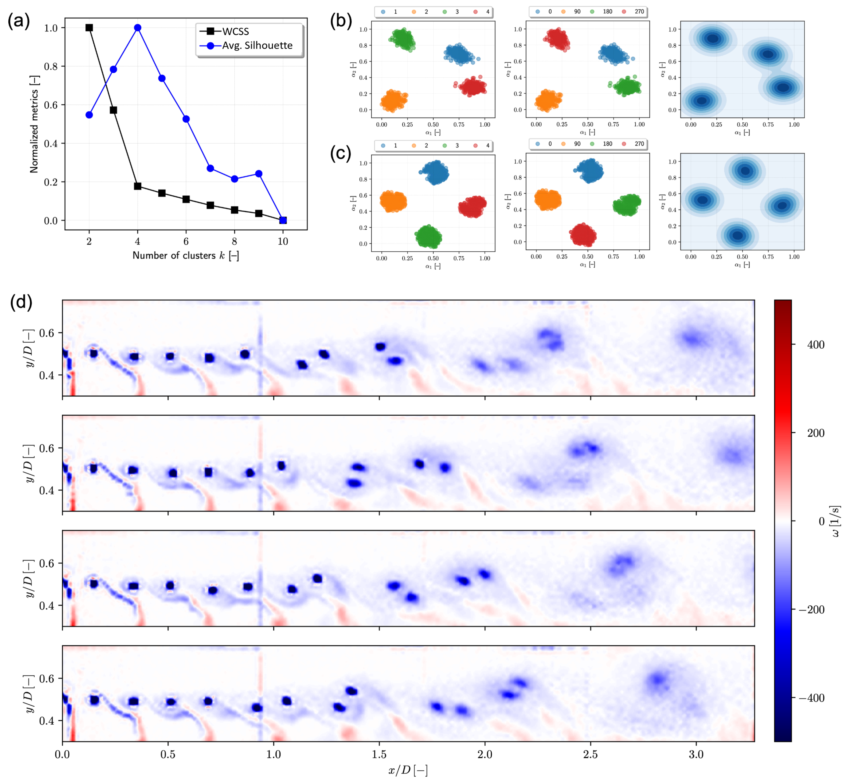
First, the k-means is applied to the whole field of view (see Figure 4). Figure 5a shows that four clusters emerge from the data set. Specifically, WCSS shows a clear elbow corresponding to $k=4$. The average silhouette exhibits a clear maximum corresponding to $k=4$. Figure 5b shows the projection of the data set onto the first two POD/PCA modes. Data are labeled both by cluster and phase, showing that the method is able to recover phase information, and the data set is clearly clustered by phase. A similar analysis and visualization is shown using t-SNE in Figure 5c, confirming the POD/PCA result. Finally, Figure 5b,c (right side) provide joint and marginal probability density functions of POD/PCA and t-SNE coefficients ${\alpha }_1$ and ${\alpha }_2$ given by KDE, confirming the data have four clusters of equal size. The corresponding cluster centroids are presented in Figure 5d, showing that the mechanism of vortex coupling and convection downstream is globally (for the large scale) deterministic throughout the investigated wake region and depends mainly on the phase. This result is consistent with the literature (see, e.g., [8]) and further strengthens the conjecture that the far-field evolution of the propeller wake structures exhibits a deterministic behavior at the macro-scale and a chaotic nature at the micro-scale.

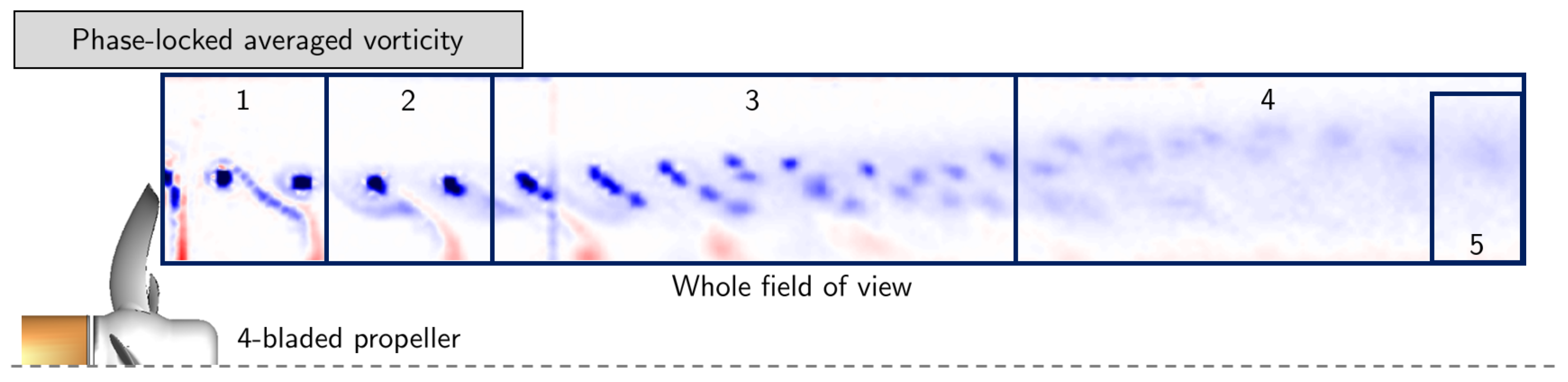
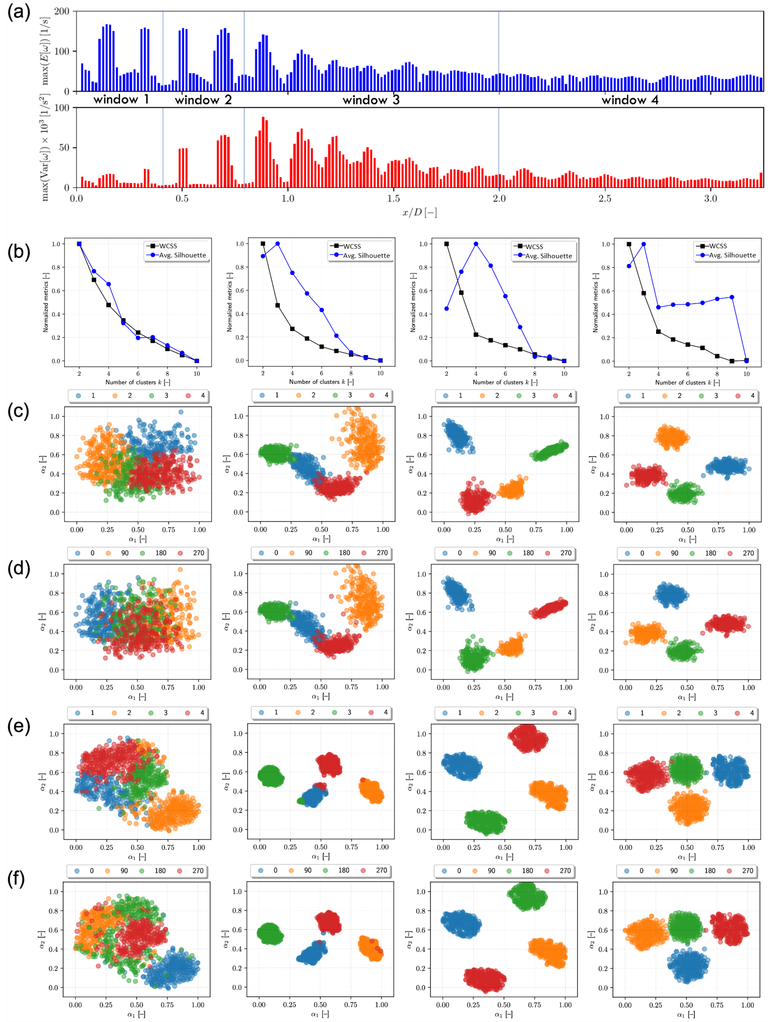
A second analysis is performed, dividing the field of view into several windows (local region of flow field), based on the vorticity mean and variance associated with each cross-section. Figure 6a shows the maximum mean and variance of cross-sections along the propeller axis. Four windows are selected, as shown in Figure 6a: (1) $0\le x/D<0.4$, where the maximum variance is low and the wake is stable; (2) $0.4\le x/D<0.8$, where the maximum variance starts increasing and the wake destabilizes; (3) $0.8\le x/D<2$, where the maximum variance reaches its own maximum and starts decreasing along with the maximum mean and the wake experiences a fully developed tip vortex interaction; (4) $2\le x/D\le 3.3$, where variance and mean are almost constant and a fully turbulent wake is observed. This second analysis is used to investigate if global wake behaviors are also present in local regions, or if the latter are dominated by some local behaviors of the wake.

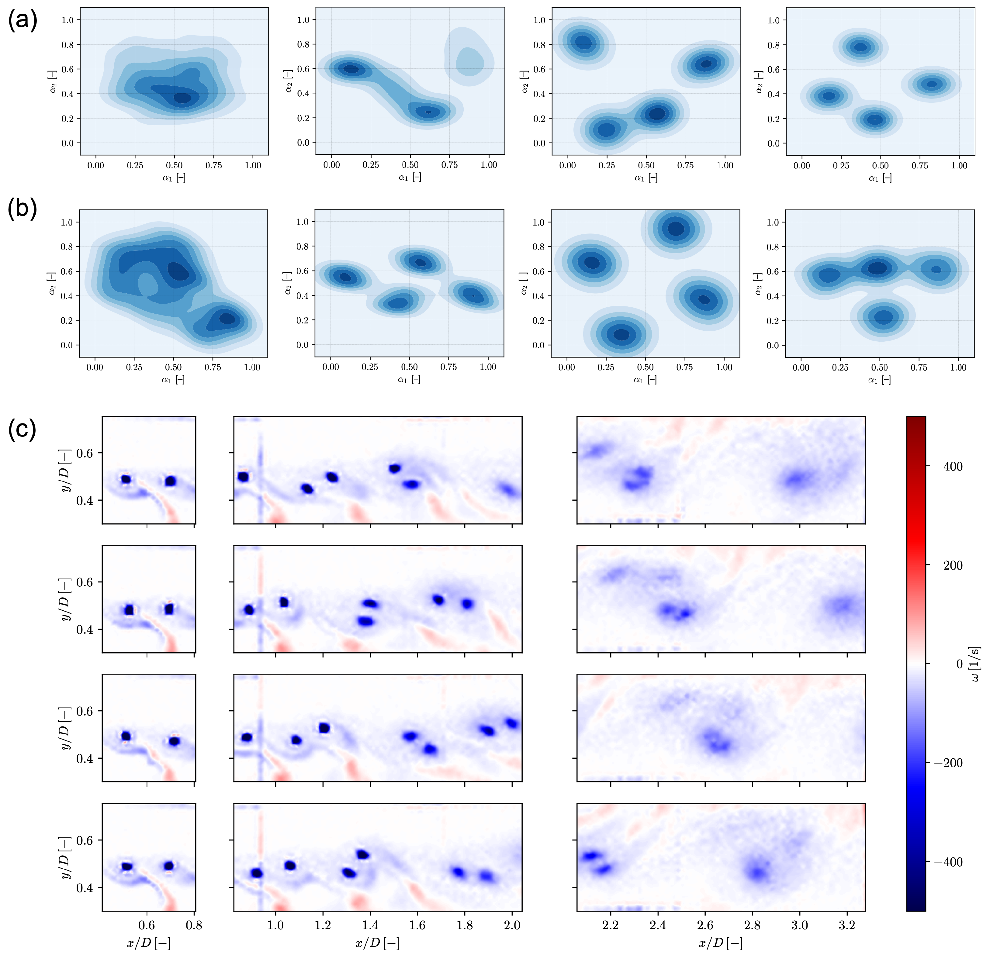
In Figure 6b, the first column, shows the WCSS and silhouette for window 1. In Figure 6c–f, the first column shows the POD/PCA (c,d) and t-SNE (e, f) coefficients labeled by cluster (c, e) and phase (d, f) for the same window. In Figure 7a,b, the first column shows the density functions of the corresponding coefficients. As expected, no significant structures are observed. The t-SNE highlights some structure and hints of data clustering. Nevertheless, these are not significant and the data can be interpreted as a single cluster. Consequently, no cluster centroid is shown in Figure 7c. Similarly, the second column of Figure 6b–f and Figure 7a,b provide the results for window 2. The clustering results are ambiguous since four and three clusters are identified by WCSS and silhouette, respectively. POD/PCA coefficients show two or three main clusters whereas the t-SNE clearly identifies four clusters associated with the propeller phases.

The results for windows 3 and 4 are presented in the third and fourth column of Figure 6b–f and Figure 7a,b, respectively, where four clusters are clearly identified with a one-to-one association to the phase. It may be noted how a high degree of determinism is still present far downstream of the propeller. It may be also noted how window 4 t-SNE analysis presents some hints of transition towards a different clustering structure. Figure 7c shows the cluster centroids associated with windows 2, 3, and 4, where rows represent clusters and columns represent windows. As discussed earlier, these centroids also represent phase-locked averages. The unsupervised association of clusters to phases by k-means indicates that the destabilization (and coupling) of tip vortices progresses following mechanisms governed by deterministic chaos.

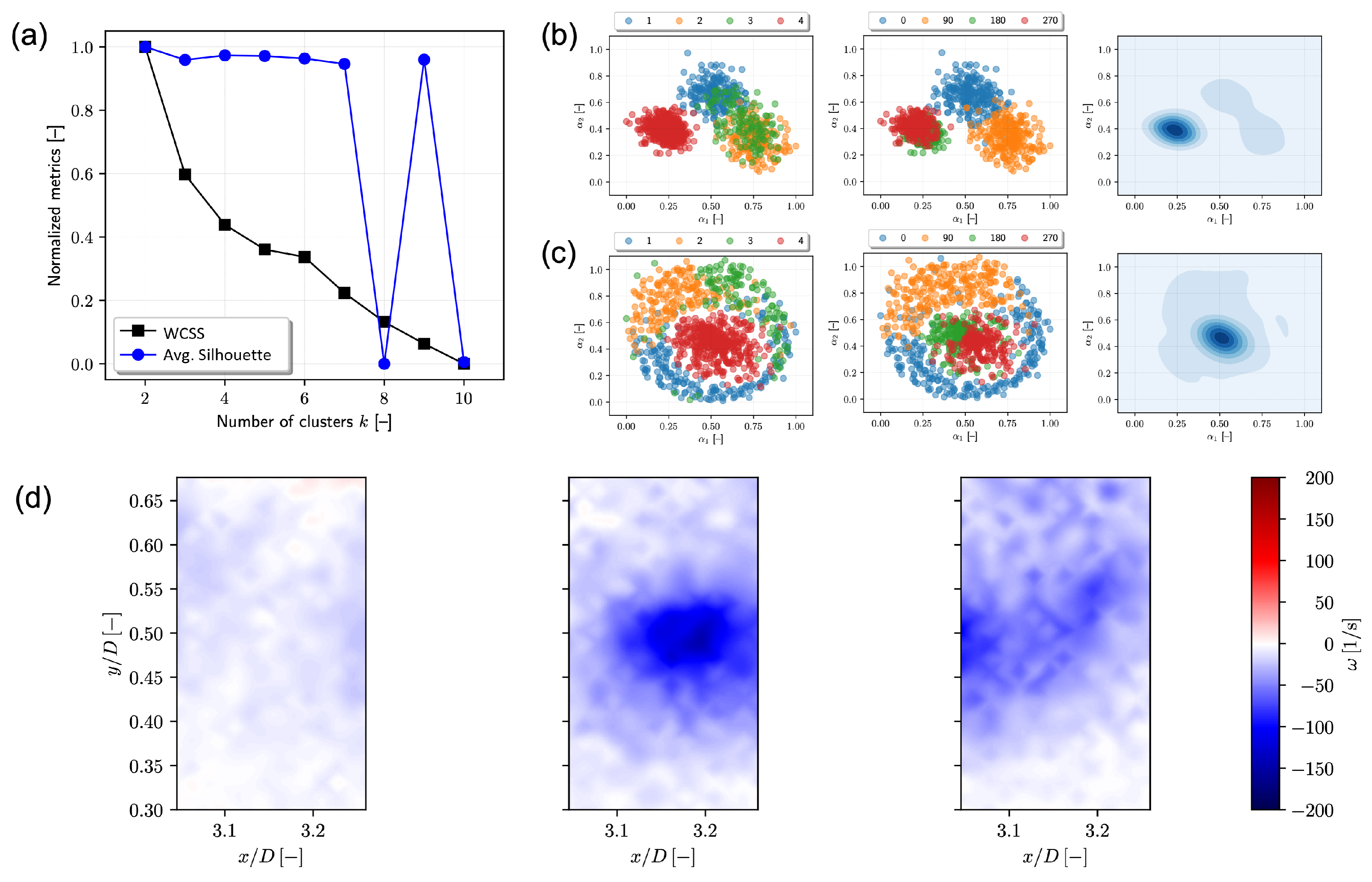
Finally, the same analysis is performed for window 5, which bounds more closely to a single vortex (see Figure 8). The clustering results are ambiguous in this region (see Figure 8a), even if some patterns are identified by both POD/PCA and t-SNE coefficients, where a pairwise mixture of phases 0–90 and 180–270 is present (see Figure 8b,c). Cluster centroids are shown in Figure 8d, where each column represents a centroid. In this case, the centroids cannot be associated with the phase-locked averages and their interpretation needs further investigation.

5. Conclusions and Future Work

A snapshot clustering approach was presented and discussed for PIV data of a 4-bladed propeller wake. Data clustering was performed using the k-means algorithm, and the optimal number of clusters was determined by evaluating two metrics: the within-cluster sum of squares and average silhouette. The focus of the snapshot clustering was on the vorticity field of the phase-locked propeller’s wake data, specifically targeting the tip vortices. To visually analyze and discuss the data clusters, a two-dimensional visualization was generated using POD/PCA, t-SNE embedding, and KDE.

The propeller wake clustering of phase-locked snapshots produced no clusters (meaning only one cluster) for the near-field data window. Clusters with a one-to-one association to the phase were found for other data windows. Specifically, this was clearly observed for the whole field of view as well as for windows covering the region where the wake transitions to unstable regimes and windows in the far field. Clustering results suggested that the wake instability and subsequent progression of tip vortices are characterized by mechanisms governed by deterministic chaos also in the far field. This result is consistent with the results of the experimental study conducted by [8], which highlights a deterministic behavior of the propeller tip vortices at the macro-scale and chaotic dynamics at the micro-scale. Finally, it can be highlighted that the use of phase-locked measurements, in combination with machine learning and data mining approaches, has allowed us to deeply investigate the propeller wake behaviors, without bothering the use of time-resolved measurements, which are definitely more challenging and expensive.

Ongoing and future work includes extending the analysis of clustering approaches to cover both spatial and temporal clustering with comparison and discussion of the results. The idea is to combine spatial/temporal clustering to fully exploits data reduction and visualization techniques to provide a physical characterization of zones and intervals in space and time domain, respectively. Furthermore, a systematic analysis of POD/PCA modes for the whole and clusterized data set will be performed. Extensions to dynamic mode decomposition [39] are also part of the ongoing research.

References

1. Frandsen, S.; Thøgersen, M.L. Integrated fatigue loading for wind turbines in wind farms by combining ambient turbulence and wakes. Wind Eng. 1999, 23, 327–339. [Google Scholar]
2. Leung, D.Y.; Yang, Y. Wind energy development and its environmental impact: A review. Renew. Sustain. Energy Rev. 2012, 16, 1031–1039. [Google Scholar] [CrossRef]
3. Stevens, R.; Meneveau, C. Flow structure and turbulence in wind farms. Annu. Rev. Fluid Mech. 2017, 49, 311–339. [Google Scholar] [CrossRef]
4. Felli, M.; Camussi, R.; Di Felice, F. Mechanisms of evolution of the propeller wake in the transition and far fields. J. Fluid Mech. 2011, 682, 5–53. [Google Scholar] [CrossRef] [Green Version]
5. Felli, M.; Falchi, M. A parametric survey of propeller wake instability mechanisms by detailed flow measurement and time resolved visualizations. In Proceedings of the 32nd Symposium on Naval Hydrodynamics, Hamburg, Germany, 5–10 August 2018. [Google Scholar]
6. Widnall, S.E. The stability of a helical vortex filament. J. Fluid Mech. 1972, 54, 641–663. [Google Scholar] [CrossRef]
7. Okulov, V. On the stability of multiple helical vortices. J. Fluid Mech. 2004, 521, 319–342. [Google Scholar] [CrossRef]
8. Felli, M.; Falchi, M. Propeller tip and hub vortex dynamic from the near to the very far field by time-resolved PIV measurements. In Proceedings of the the 33rd Symposium on Naval Hydrodynamics, Osaka, Japan, 18–23 October 2020. [Google Scholar]
9. Wang, L.; Martin, J.E.; Felli, M.; Carrica, P.M. Experiments and CFD for the propeller wake of a generic submarine operating near the surface. Ocean Eng. 2020, 206, 107304. [Google Scholar] [CrossRef]
10. Felli, M.; Falchi, M.; Pereira, F.J.A. Distance effect on the behavior of an impinging swirling jet by PIV and flow visualizations. Exp. Fluids 2010, 48, 197–209. [Google Scholar] [CrossRef]
11. Felli, M.; Falchi, M. Propeller wake evolution mechanisms in oblique flow conditions. J. Fluid Mech. 2018, 845, 520–559. [Google Scholar] [CrossRef]
12. Berkooz, G.; Holmes, P.; Lumley, J.L. The proper orthogonal decomposition in the analysis of turbulent flows. Annu. Rev. Fluid Mech. 1993, 25, 539–575. [Google Scholar] [CrossRef]
13. Gordeyev, S.V.; Thomas, F.O. Coherent structure in the turbulent planar jet. Part 2. Structural topology via POD eigenmode projection. J. Fluid Mech. 2002, 460, 349–380. [Google Scholar] [CrossRef] [Green Version]
14. Zhou, X.; Hitt, D.L. Proper orthogonal decomposition analysis of coherent structures in a transient buoyant jet. J. Turbul. 2004, 5, N28. [Google Scholar] [CrossRef]
15. Serani, A.; Durante, D.; Diez, M.; D’Agostino, D.; Clement, S.; Badra, J.; Andre, M.; Habukawa, M.; Bardet, P. PIV Data Clustering of a Buoyant Jet in a Stratified Environment. In Proceedings of the 57th AIAA Aerospace Sciences Meeting, SciTech 2019, San Diego, CA, USA, 7–11 January 2019. [Google Scholar]
16. Barwey, S.; Raman, V.; Steinberg, A.M. Data-Driven Reduction and Decomposition via Time-Axis Clustering. In Proceedings of the AIAA Scitech 2020 Forum, Orlando, FL, USA, 6–10 January 2020; p. 0365. [Google Scholar]
17. Van der Maaten, L.; Hinton, G. Visualizing data using t-SNE. J. Mach. Learn. Res. 2008, 9, 2579–2605. [Google Scholar]
18. Wu, J.; Wang, J.; Xiao, H.; Ling, J. Visualization of high dimensional turbulence simulation data using t-SNE. In Proceedings of the 19th AIAA Non-Deterministic Approaches Conference, Grapevine, TX, USA, 9–13 January 2017; p. 1770. [Google Scholar]
19. Perceau, M.; Guibert, P.; Guilain, S. Analysis of a tumbling motion using a clustering algorithm on dual-PIV measurements: Application to the in-cylinder flow of a Miller cycle engine. Exp. Fluids 2022, 63, 54. [Google Scholar] [CrossRef]
20. Calvet, A.G.; Dave, M.; Franck, J.A. Unsupervised clustering and performance prediction of vortex wakes from bio-inspired propulsors. Bioinspiration Biomim. 2021, 16, 046015. [Google Scholar] [CrossRef]
21. Doijode, P.S.; Hickel, S.; van Terwisga, T.; Visser, K. A machine learning approach for propeller design and optimization: Part I. Appl. Ocean Res. 2022, 124, 103178. [Google Scholar] [CrossRef]
22. Sharma, R.; Simula, T.P. Machine-learning classification of two-dimensional vortex configurations. Phys. Rev. A 2022, 105, 033301. [Google Scholar] [CrossRef]
23. Felli, M.; Falchi, M.; Dubbioso, G. Tomographic-PIV survey of the near-field hydrodynamic and hydroacoustic characteristics of a marine propeller. J. Ship Res. 2015, 59, 201–208. [Google Scholar] [CrossRef]
24. Posa, A.; Broglia, R.; Felli, M.; Falchi, M.; Balaras, E. Characterization of the wake of a submarine propeller via Large-Eddy simulation. Comput. Fluids 2019, 184, 138–152. [Google Scholar] [CrossRef]
25. Scarano, F. Iterative image deformation methods in PIV. Meas. Sci. Technol. 2001, 13, R1. [Google Scholar] [CrossRef]
26. Jain, A.K. Data clustering: 50 years beyond K-means. Pattern Recognit. Lett. 2010, 31, 651–666. [Google Scholar] [CrossRef]
27. Drineas, P.; Frieze, A.; Kannan, R.; Vempala, S.; Vinay, V. Clustering large graphs via the singular value decomposition. Mach. Learn. 2004, 56, 9–33. [Google Scholar] [CrossRef] [Green Version]
28. Lloyd, S. Least squares quantization in PCM. IEEE Trans. Inf. Theory 1982, 28, 129–137. [Google Scholar] [CrossRef] [Green Version]
29. Arthur, D.; Vassilvitskii, S. k-means++: The advantages of careful seeding. In Proceedings of the eighteenth annual ACM-SIAM symposium on Discrete algorithms, New Orleans, LA, USA, 7–9 January; Society for Industrial and Applied Mathematics: Philadelphia, PA, USA, 2007; pp. 1027–1035. [Google Scholar]
30. Bishop, C.M. Pattern Recognition and Machine Learning (Information Science and Statistics); Springer: Secaucus, NJ, USA, 2006. [Google Scholar]
31. Golub, G.H.; Reinsch, C. Singular value decomposition and least squares solutions. Numer. Math. 1970, 14, 403–420. [Google Scholar] [CrossRef]
32. Cizmas, P.G.; Palacios, A.; O’Brien, T.; Syamlal, M. Proper-orthogonal decomposition of spatio-temporal patterns in fluidized beds. Chem. Eng. Sci. 2003, 58, 4417–4427. [Google Scholar] [CrossRef]
33. Holmes, P.; Lumley, J.L.; Berkooz, G.; Rowley, C.W. Turbulence, Coherent Structures, Dynamical Systems and Symmetry; Cambridge University Press: Cambridge, UK, 2012. [Google Scholar]
34. Silverman, B.W. Density Estimation for Statistics and Data Analysis; Routledge: Abingdon-on-Thames, UK, 2018. [Google Scholar]
35. Simonoff, J.S. Smoothing Methods in Statistics; Springer Science & Business Media: Berlin/Heidelberg, Germany, 2012. [Google Scholar]
36. Ketchen, D.J.; Shook, C.L. The application of cluster analysis in strategic management research: An analysis and critique. Strateg. Manag. J. 1996, 17, 441–458. [Google Scholar] [CrossRef]
37. Rousseeuw, P.J. Silhouettes: A graphical aid to the interpretation and validation of cluster analysis. J. Comput. Appl. Math. 1987, 20, 53–65. [Google Scholar] [CrossRef] [Green Version]
38. Pedregosa, F.; Varoquaux, G.; Gramfort, A.; Michel, V.; Thirion, B.; Grisel, O.; Blondel, M.; Prettenhofer, P.; Weiss, R.; Dubourg, V.; et al. Scikit-learn: Machine Learning in Python. J. Mach. Learn. Res. 2011, 12, 2825–2830. [Google Scholar]
39. Kutz, J.N.; Brunton, S.L.; Brunton, B.W.; Proctor, J.L. Dynamic Mode Decomposition: Data-Driven Modeling of Complex Systems; SIAM: Philadelphia, PA, USA, 2016. [Google Scholar]
Figure 1. Snapshot of a cavitating propeller.
Jmse 11 01220 g001
Figure 2. Overall machine learning and data mining workflow for propeller wake investigation.
Jmse 11 01220 g002
Figure 3. Sketch (left) and side (right) views of the PIV experimental setup.
Jmse 11 01220 g003
Figure 4. Windows used for clustering of vorticity snapshots.
Jmse 11 01220 g004
Figure 5. Whole field of view: (a) clustering metrics; (b) data-projection on the first two POD/PCA modes; and (c) embedding via t-SNE, labeled by cluster (left) and phase (center), along with joint probability density functions by KDE (right); (d) cluster centroids corresponding to phases 0, 90, 180, 270 deg (from top to bottom).
Jmse 11 01220 g005
Figure 6. Whole field of view: (a) maximum value of mean (top) and variance (bottom) of the vorticity along cross sections; (b) clustering metrics by window; and (c,d) data-projection on the first two POD/PCA modes and (e,f) embedding via t-SNE, label by cluster and phase (from left to right, windows 1, 2, 3, 4).
Jmse 11 01220 g006
Figure 7. Joint probability density functions by window of (a) POD/PCA and (b) t-SNE coefficients by KDE (from left to right, windows 1, 2, 3, and 4.); (c) cluster centroids corresponding to phases 0, 90, 180, 270 deg, for windows 2, 3, and 4 (from left to right, windows).
Jmse 11 01220 g007
Figure 8. Window 5: (a) clustering metrics; (b) data-projection on the first two POD/PCA modes; and (c) embedding via t-SNE, labeled by cluster (left) and phase (center), along with joint probability density functions by KDE centroids (right); (d) cluster centroids.
Jmse 11 01220 g008
Disclaimer/Publisher’s Note: The statements, opinions and data contained in all publications are solely those of the individual author(s) and contributor(s) and not of MDPI and/or the editor(s). MDPI and/or the editor(s) disclaim responsibility for any injury to people or property resulting from any ideas, methods, instructions or products referred to in the content.