
Multiscale Analysis and Prediction of Sea Level in the Northern South China Sea Based on Tide Gauge and Satellite Data
 , , ,
, , , 
Abstract
:1. Introduction
2. Materials and Methods
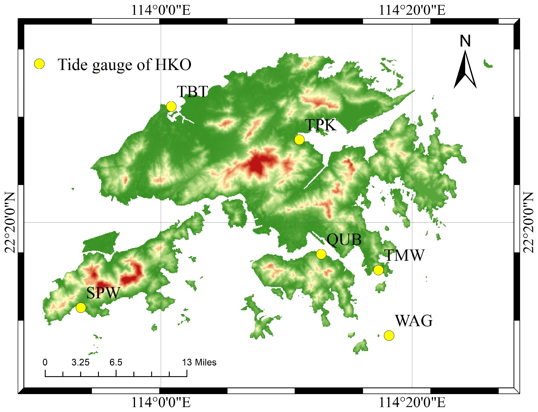
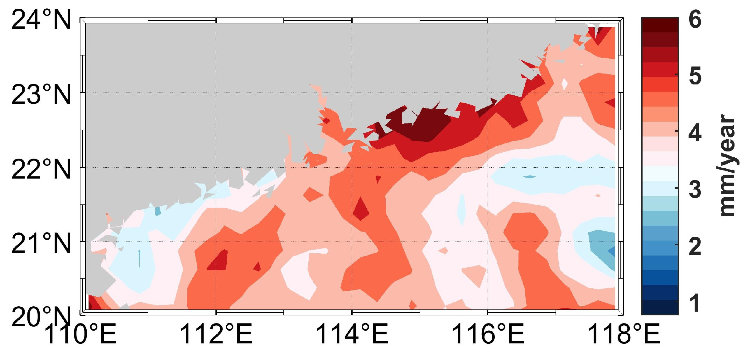
2.1. Study Area
2.2. Datasets
2.3. Data Preprocessing
2.4. Methods
2.4.1. Ensemble Empirical Mode Decomposition (EEMD)
2.4.2. Multifractal Detrended Fluctuation Analysis (MF-DFA)
2.4.3. Long Short-Term Memory (LSTM) Neural Network
3. Results and Discussion
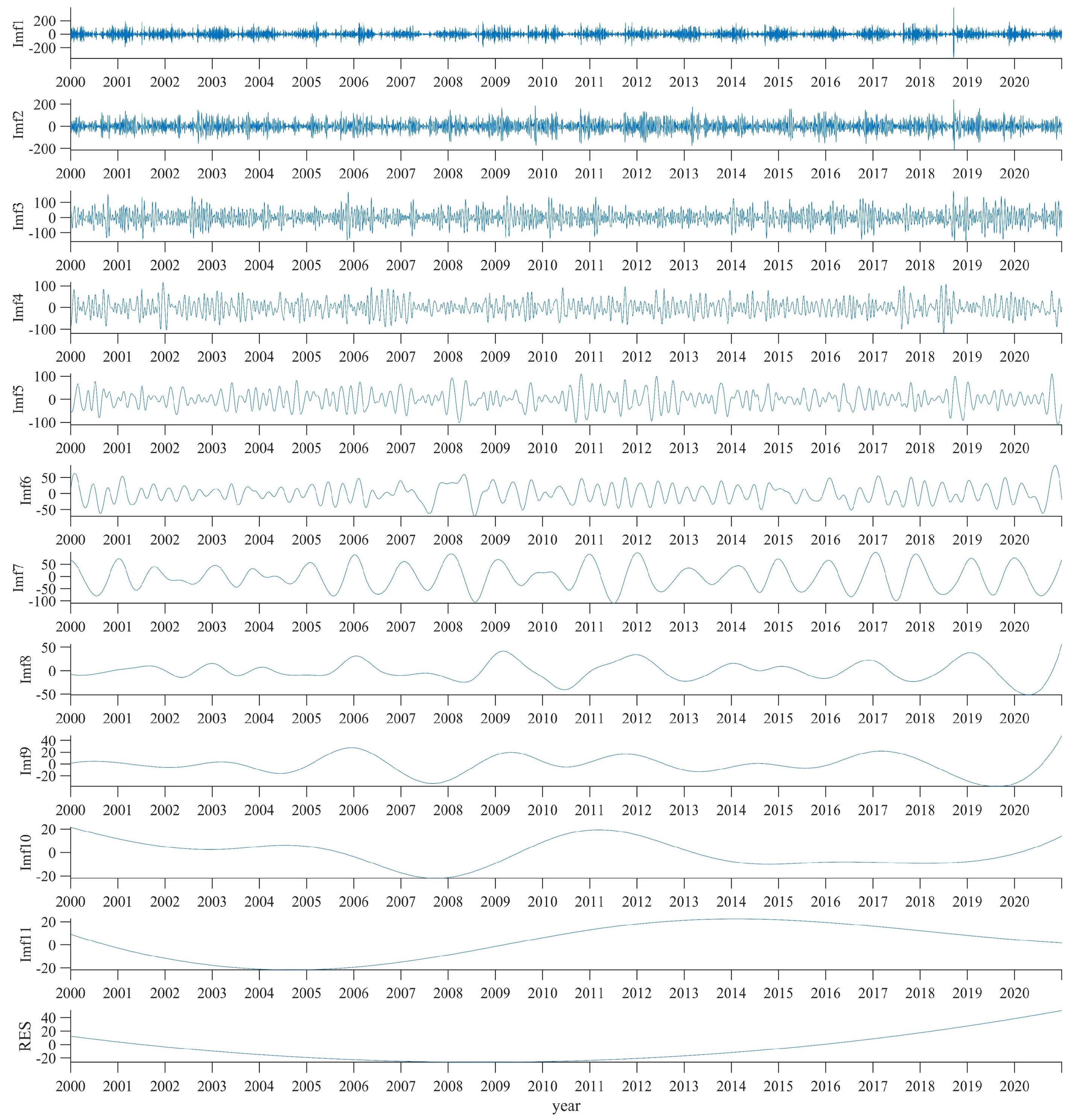
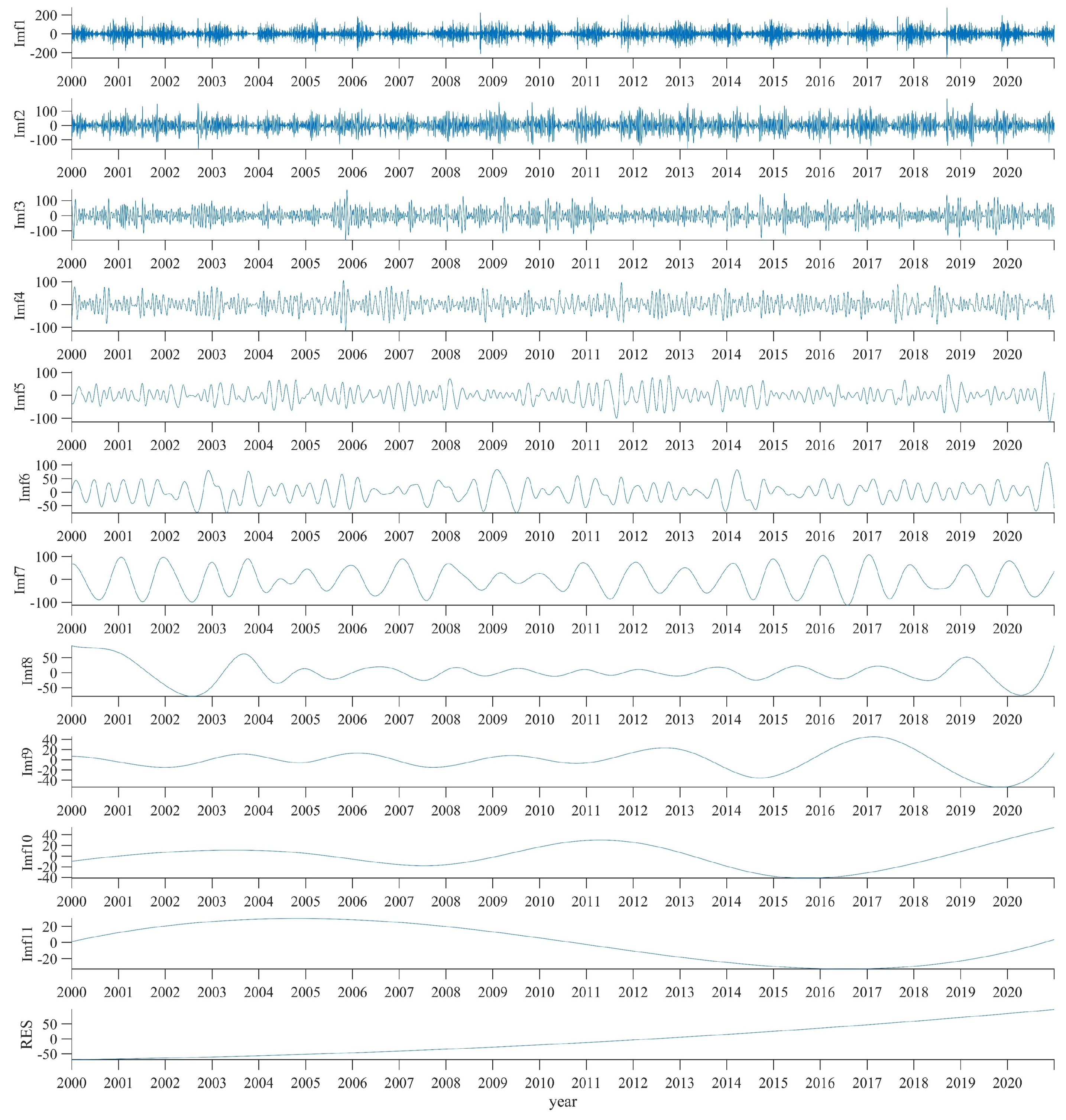
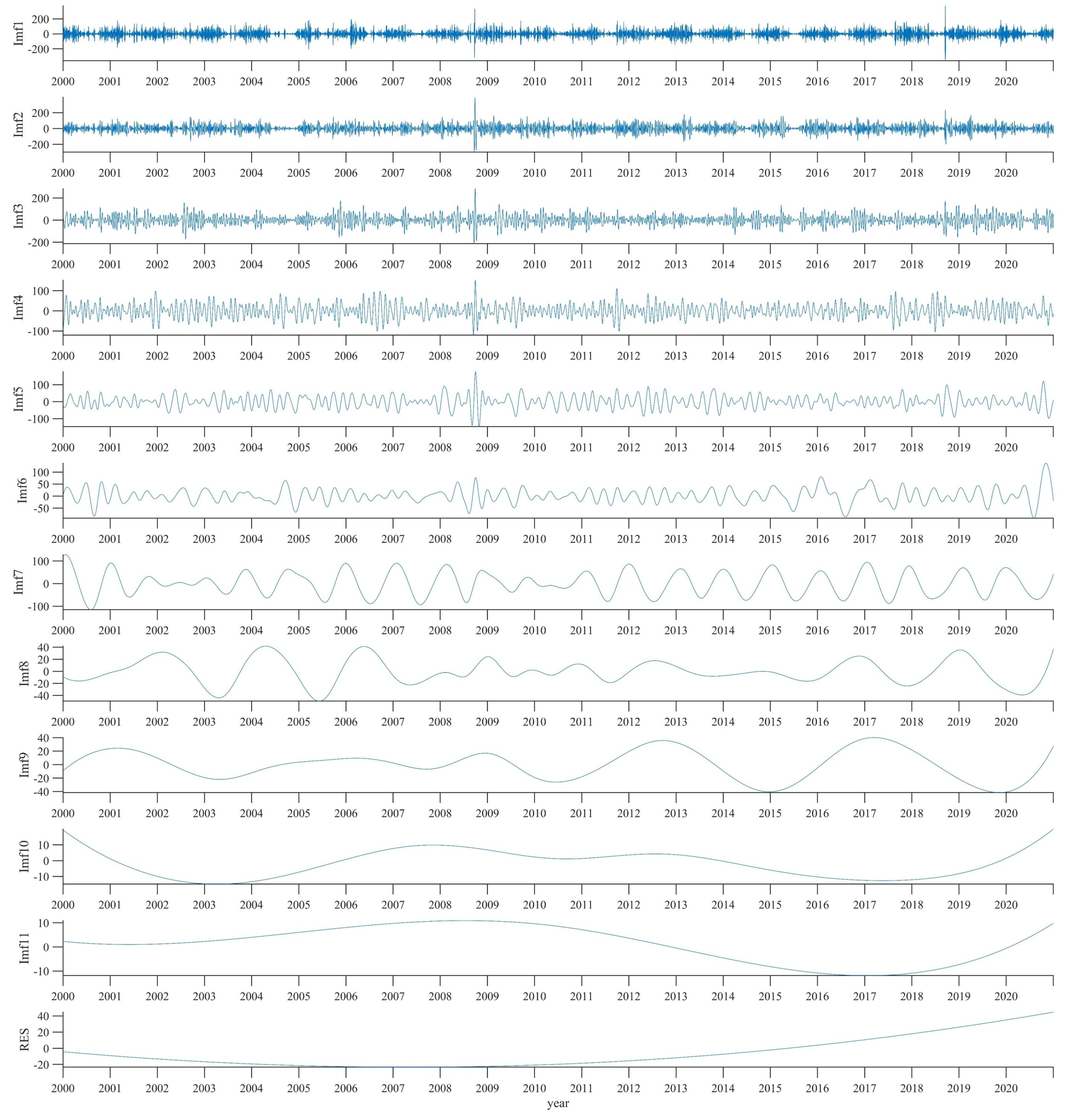
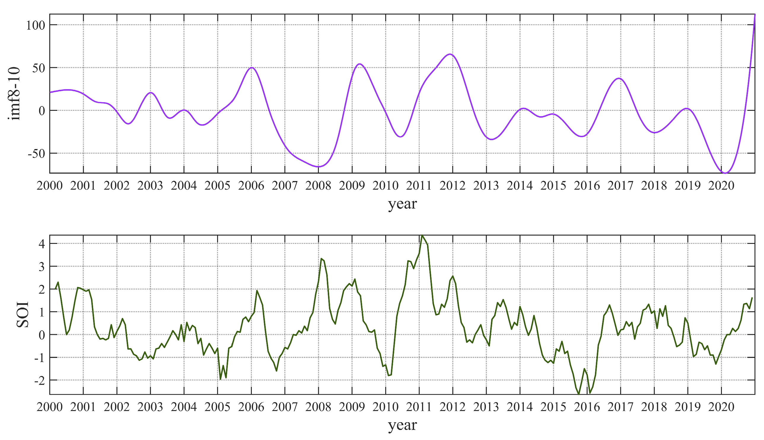
3.1. EEMD Analysis Results
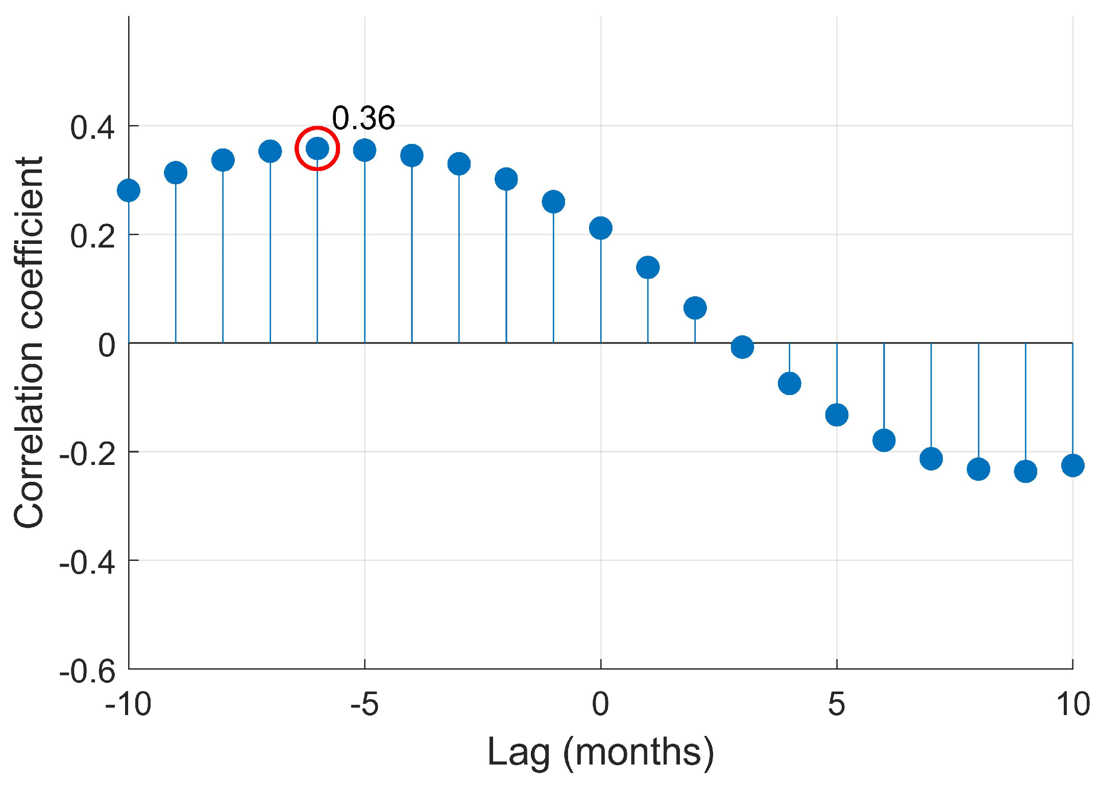
3.2. Analysis of the Impact of ENSO on Sea-Level Change
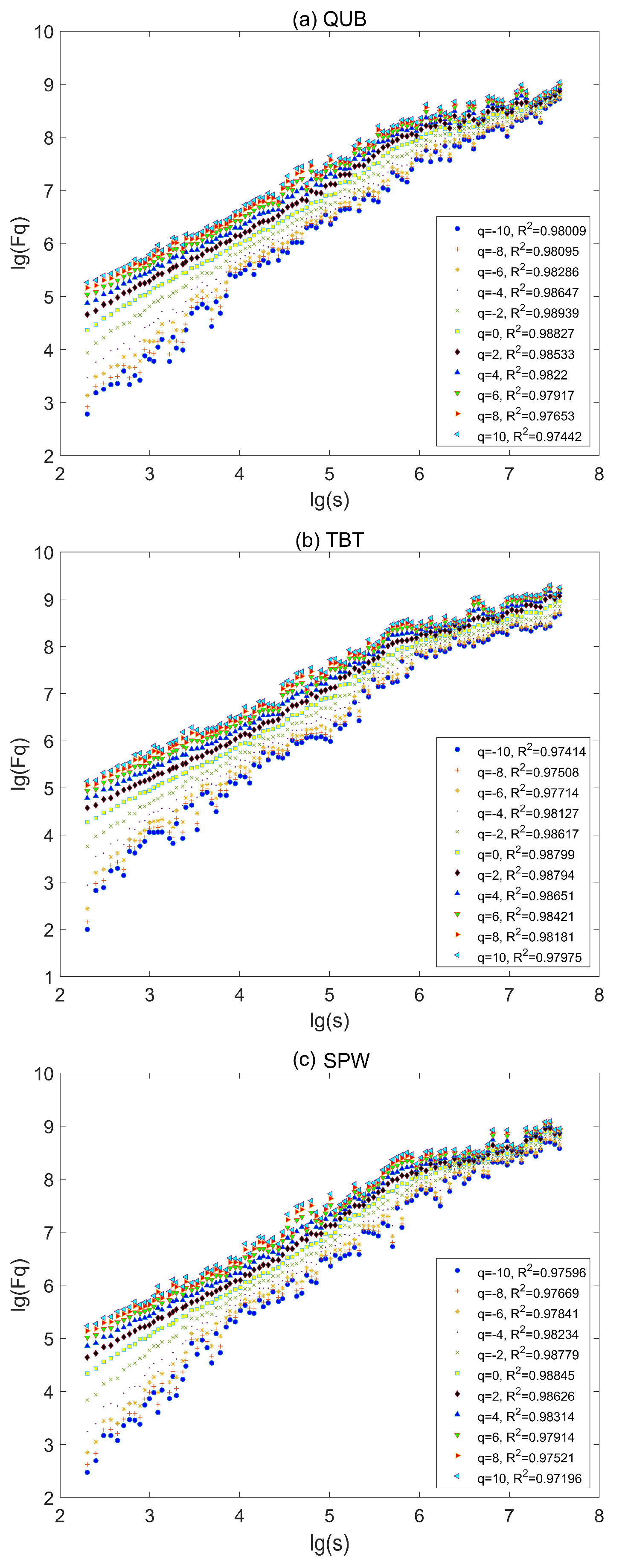
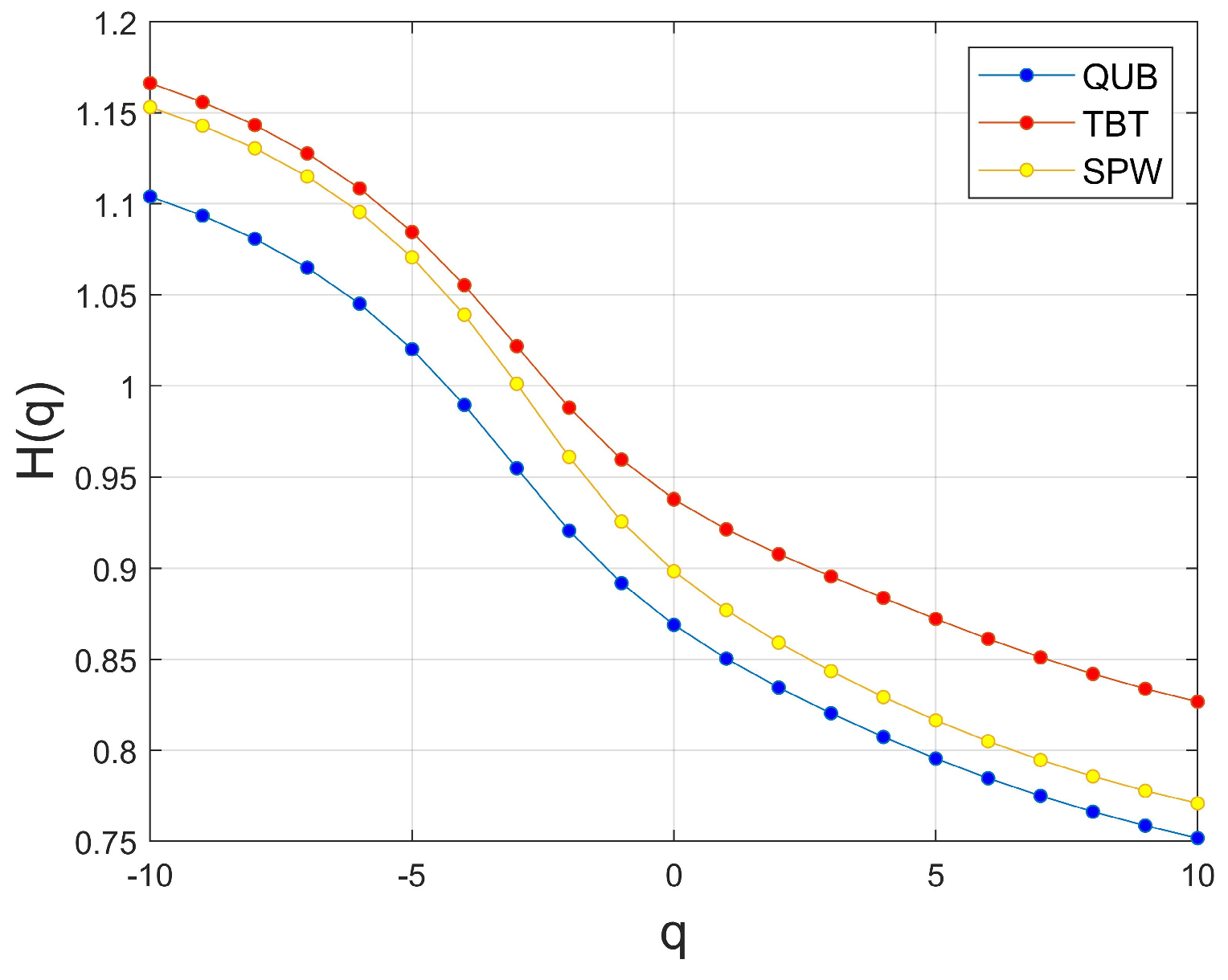
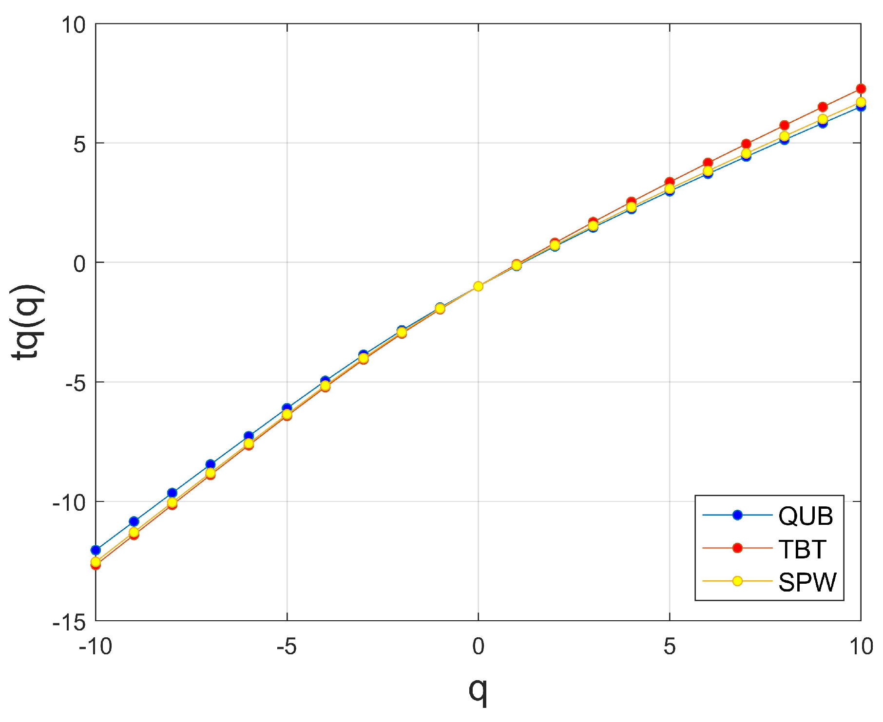
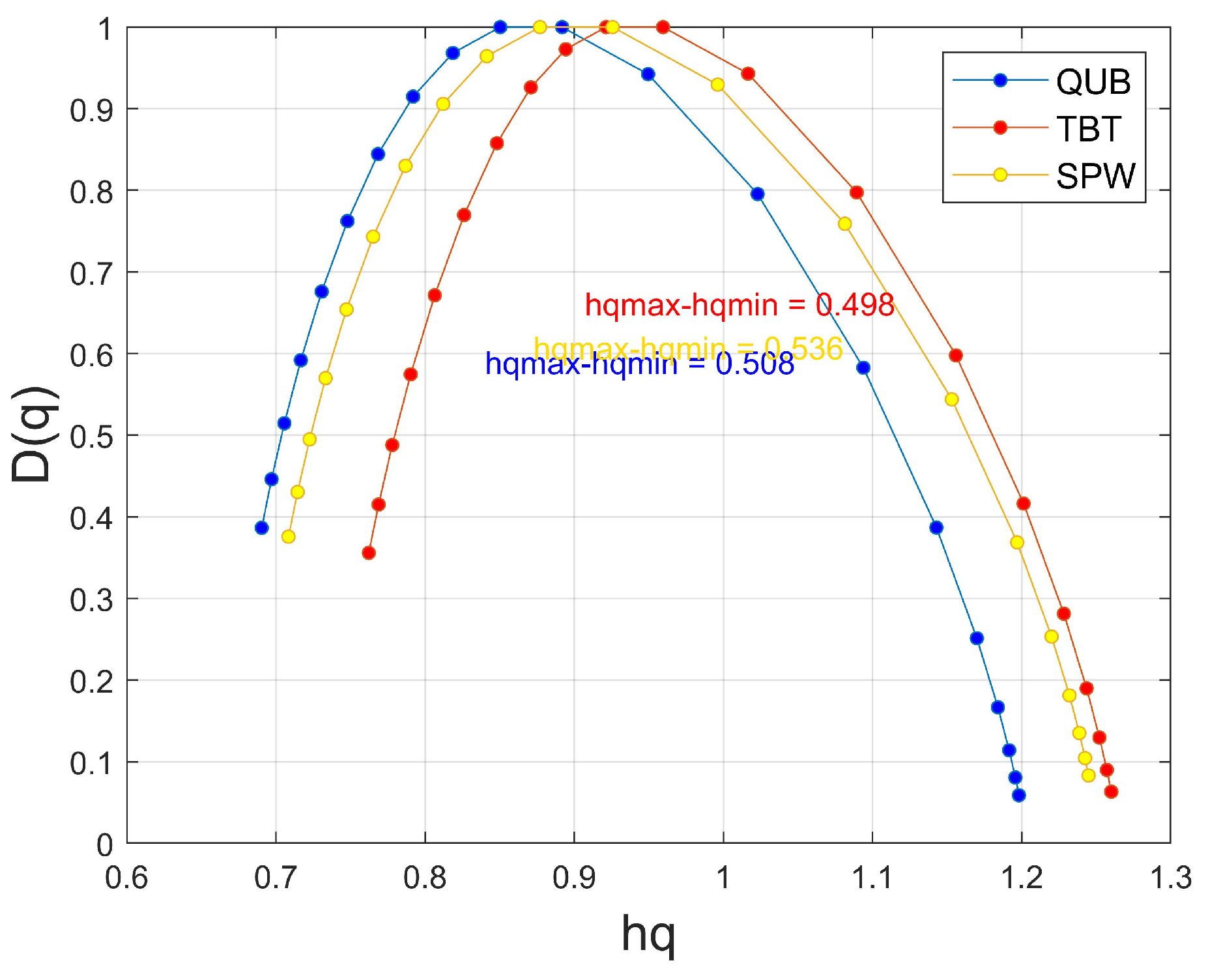
3.3. MF-DFA Analysis Results
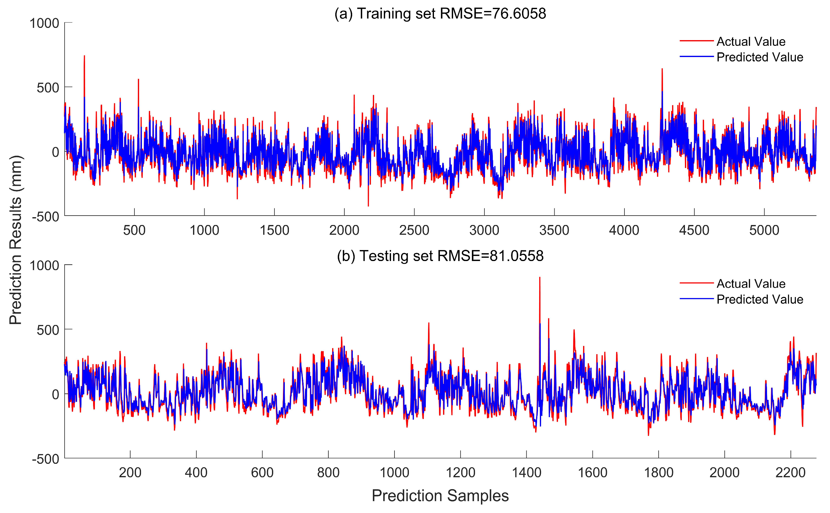
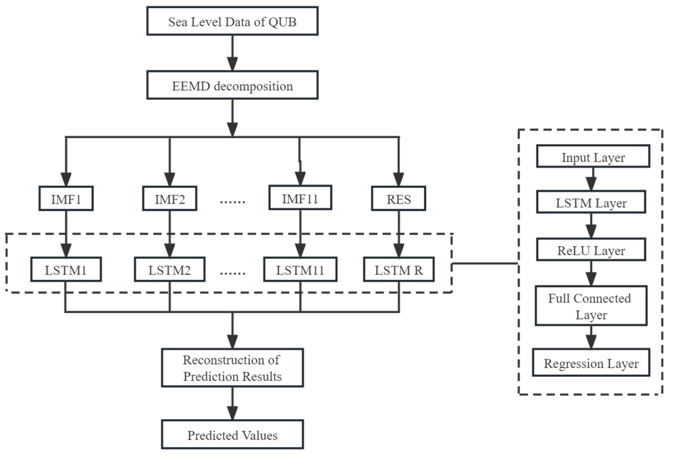
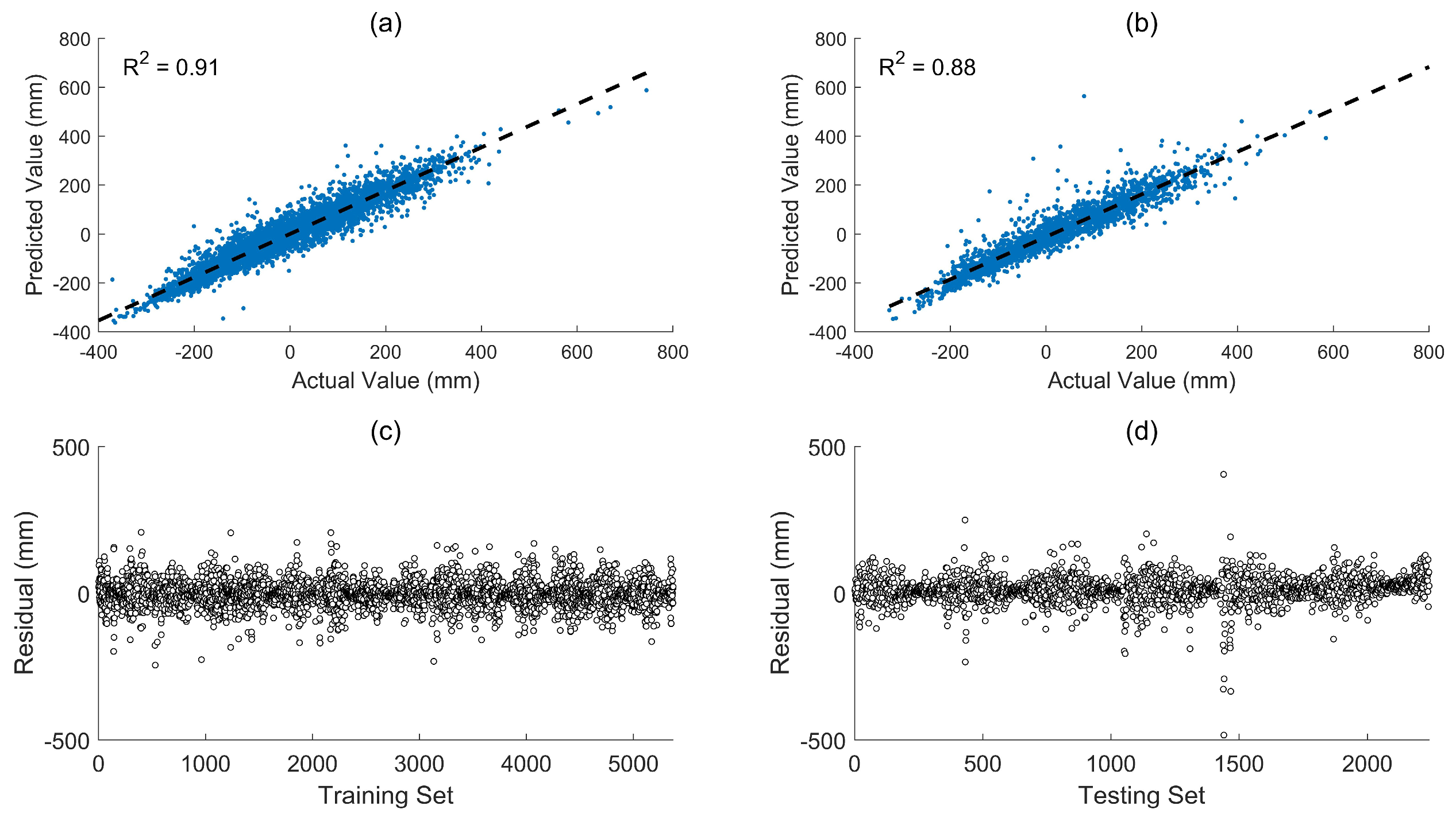
3.4. Prediction of Sea Level in the Northern South China Sea Based on EEMD-LSTM
4. Conclusions
Author Contributions
Funding
Institutional Review Board Statement
Informed Consent Statement
Data Availability Statement
Acknowledgments
Conflicts of Interest
References
- Merrifield, M.A.; Merrifield, S.T.; Mitchum, G.T. An Anomalous Recent Acceleration of Global Sea Level Rise. J. Clim. 2009, 22, 5772–5781. [Google Scholar] [CrossRef] [Green Version]
- Frederikse, T.; Landerer, F.; Caron, L.; Adhikari, S.; Parkes, D.; Humphrey, V.W.; Dangendorf, S.; Hogarth, P.; Zanna, L.; Cheng, L. The causes of sea-level rise since 1900. Nature 2020, 584, 393–397. [Google Scholar] [CrossRef] [PubMed]
- Church, J.A.; White, N.J. Sea-Level Rise from the Late 19th to the Early 21st Century. Surv. Geophys. 2011, 32, 585–602. [Google Scholar] [CrossRef] [Green Version]
- Masson-Delmotte, V.; Zhai, P.; Pirani, A.; Connors, S.L.; Péan, C.; Berger, S.; Caud, N.; Chen, Y.; Goldfarb, L.; Gomis, M. IPCC Climate Change 2021: The Physical Science Basis. Contribution of Working Group I to the Sixth Assessment Report of the Intergovernmental Panel on Climate Change; Cambridge University Press: Cambridge, UK, 2021. [Google Scholar]
- Ericson, J.; Vorosmarty, C.; Dingman, S.; Ward, L.; Meybeck, M. Effective sea-level rise and deltas: Causes of change and human dimension implications. Glob. Planet. Change 2006, 50, 63–82. [Google Scholar] [CrossRef]
- Duke, N.C.; Meynecke, J.O.; Dittmann, S.; Ellison, A.M.; Anger, K.; Berger, U.; Cannicci, S.; Diele, K.; Ewel, K.C.; Field, C.D. A world without mangroves? Science 2007, 317, 41–42. [Google Scholar] [CrossRef] [Green Version]
- Nicholls, R.J.; Hoozemans, F.M.J.; Marchand, M. Increasing food risk and wetland losses due to global sea-level rise: Regional and global analyses. Glob. Environ. Change 1999, 9, S69–S87. [Google Scholar] [CrossRef]
- Huang, Z.; Zong, Y.; Zhang, W. Coastal Inundation due to Sea Level Rise in the Pearl River Delta, China. Nat. Hazards 2004, 33, 247–264. [Google Scholar] [CrossRef] [Green Version]
- Woodruff, J.D.; Irish, J.L.; Camargo, S.J. Coastal flooding by tropical cyclones and sea-level rise. Nature 2013, 504, 44–52. [Google Scholar] [CrossRef] [Green Version]
- Stammer, D.; Cazenave, A.; Ponte, R.M.; Tamisiea, M.E. Causes for contemporary regional sea level changes. Annu. Rev. Mar. Sci. 2013, 5, 21–46. [Google Scholar] [CrossRef] [Green Version]
- Cheng, X.; Qi, Y. Trends of sea level variations in the South China Sea from merged altimetry data. Glob. Planet. Change 2007, 57, 371–382. [Google Scholar] [CrossRef]
- Fang, G.; Chen, H.; Wei, Z.; Wang, Y.; Wang, X.; Li, C. Trends and interannual variability of the South China Sea surface winds, surface height, and surface temperature in the recent decade. J. Geophys. Res. Ocean. 2006, 111, D17301. [Google Scholar] [CrossRef] [Green Version]
- Peng, D.; Palanisamy, H.; Cazenave, A.; Meyssignac, B. Interannual Sea Level Variations in the South China Sea Over 1950–2009. Mar. Geod. 2013, 36, 164–182. [Google Scholar] [CrossRef]
- Wang, L.; Li, Q.; Bi, H.; Mao, X.Z. Human impacts and changes in the coastal waters of south China. Sci. Total Environ. 2016, 562, 108–114. [Google Scholar] [CrossRef] [PubMed]
- Ablain, M.; Legeais, J.F.; Prandi, P.; Marcos, M.; Fenoglio-Marc, L.; Dieng, H.B.; Benveniste, J.; Cazenave, A. Satellite Altimetry-Based Sea Level at Global and Regional Scales. Surv. Geophys. 2017, 38, 7–31. [Google Scholar] [CrossRef]
- Gregory, J.M.; Church, J.A.; Boer, G.J.; Dixon, K.W.; Flato, G.M.; Jackett, D.R.; Lowe, J.A.; O’Farrell, S.P.; Roeckner, E.; Russell, G.L.; et al. Comparison of results from several AOGCMs for global and regional sea-level change 1900–2100. Clim. Dyn. 2001, 18, 225–240. [Google Scholar] [CrossRef]
- Liu, S.; Chen, C.; Liu, K.; Mu, L.; Wang, H.; Wu, X.; Zhang, J.; Duan, X.; Gao, J. Vertical motions of tide gauge stations near the Bohai Sea and Yellow Sea. Sci. China Earth Sci. 2015, 58, 2279–2288. [Google Scholar] [CrossRef]
- Wang, L.; Li, Q.; Mao, X.-z.; Bi, H.; Yin, P. Interannual sea level variability in the Pearl River Estuary and its response to El Niño–Southern Oscillation. Glob. Planet. Change 2018, 162, 163–174. [Google Scholar] [CrossRef]
- Willis, J.K.; Chambers, D.P.; Nerem, R.S. Assessing the globally averaged sea level budget on seasonal to interannual timescales. J. Geophys. Res. Ocean. 2008, 113, C06015. [Google Scholar] [CrossRef] [Green Version]
- Department of marine early warning and monitoring. 2020 China Sea Level Bulletin; The Ministry of Natural Resources: Beijing, China, 2021. [Google Scholar]
- Dangendorf, S.; Frederikse, T.; Chafik, L.; Klinck, J.M.; Ezer, T.; Hamlington, B.D. Data-driven reconstruction reveals large-scale ocean circulation control on coastal sea level. Nat. Clim. Change 2021, 11, 514–520. [Google Scholar] [CrossRef]
- Cheng, Y.; Plag, H.-P.; Hamlington, B.D.; Xu, Q.; He, Y. Regional sea level variability in the bohai sea, yellow sea, and east china sea. Cont. Shelf Res. 2015, 111, 95–107. [Google Scholar] [CrossRef]
- Milne, G.A.; Gehrels, W.R.; Hughes, C.W.; Tamisiea, M.E. Identifying the causes of sea-level change. Nat. Geosci. 2009, 2, 471–478. [Google Scholar] [CrossRef] [Green Version]
- Cazenave, A.; Llovel, W. Contemporary sea level rise. Annu. Rev. Mar. Sci. 2010, 2, 145–173. [Google Scholar] [CrossRef] [PubMed] [Green Version]
- Qu, Y.; Jevrejeva, S.; Jackson, L.P.; Moore, J.C. Coastal Sea level rise around the China Seas. Glob. Planet. Change 2019, 172, 454–463. [Google Scholar] [CrossRef]
- He, L.; Li, G.; Li, K.; Shu, Y. Estimation of regional sea level change in the Pearl River Delta from tide gauge and satellite altimetry data. Estuarine, Coast. Shelf Sci. 2014, 141, 69–77. [Google Scholar] [CrossRef]
- Ding, X.; Zheng, D.; Chen, Y.; Chao, J.; Li, Z. Sea level change in Hong Kong from tide gauge measurements of 1954-1999. J. Geod. 2001, 74, 683–689. [Google Scholar] [CrossRef]
- Cabanes, C. Sea Level Rise During Past 40 Years Determined from Satellite and in Situ Observations. Science 2001, 294, 840–842. [Google Scholar] [CrossRef] [Green Version]
- Willis, J.K.; Roemmich, D.; Cornuelle, B. Interannual variability in upper ocean heat content, temperature, and thermosteric expansion on global scales. J. Geophys. Res. Ocean. 2004, 109, 840–842. [Google Scholar] [CrossRef] [Green Version]
- Ho, C.R.; Zheng, Q.; Soong, Y.S.; Kuo, N.J.; Hu, J.H. Seasonal variability of sea surface height in the South China Sea observed with TOPEX/Poseidon altimeter data. J. Geophys. Res. Atmos. 2000, 105, 13981–13990. [Google Scholar] [CrossRef]
- Li, L.; Jindian, X.; Rongshuo, C. Trends of sea level rise in the South China Sea during the 1990s: An altimetry result. Chin. Sci. Bull. 2002, 47, 582–585. [Google Scholar] [CrossRef]
- Vivier, F.; Kelly, K.A.; Harismendy, M. Causes of large-scale sea level variations in the Southern Ocean: Analyses of sea level and a barotropic model. J. Geophys. Res. Ocean. 2005, 110, C09014. [Google Scholar] [CrossRef] [Green Version]
- Rong, Z.; Liu, Y.; Zong, H.; Cheng, Y. Interannual sea level variability in the South China Sea and its response to ENSO. Glob. Planet. Change 2007, 55, 257–272. [Google Scholar] [CrossRef]
- Cheng, Y.; Hamlington, B.D.; Plag, H.-P.; Xu, Q. Influence of ENSO on the variation of annual sea level cycle in the South China Sea. Ocean Eng. 2016, 126, 343–352. [Google Scholar] [CrossRef]
- Liu, C.; Li, X.; Wang, S.; Tang, D.; Zhu, D. Interannual variability and trends in sea surface temperature, sea surface wind, and sea level anomaly in the South China Sea. Int. J. Remote Sens. 2020, 41, 4160–4173. [Google Scholar] [CrossRef]
- Hebrard, E.; Llovel, W.; Cazenave, A.; Rogel, P. Interannual to multidecadal variability of the mean sea level. In Proceedings of the AGU Fall Meeting Abstracts, San Francisco, CA, USA, 11–15 December 2008; pp. 33–1347. [Google Scholar]
- Tomasicchio, G.R.; Lusito, L.; D’Alessandro, F.; Frega, F.; Francone, A.; De Bartolo, S. A direct scaling analysis for the sea level rise. Stoch. Environ. Res. Risk Assess. 2018, 32, 3397–3408. [Google Scholar] [CrossRef]
- Huang, N.E.; Shen, Z.; Long, S.R.; Wu, M.C.; Shih, H.H.; Zheng, Q.; Yen, N.C.; Tung, C.C.; Liu, H.H. The empirical mode decomposition and the Hilbert spectrum for nonlinear and non-stationary time series analysis. Proc. Math. Phys. Eng. Sci. 1998, 454, 903–995. [Google Scholar] [CrossRef]
- Wu, Z.; Huang, N.E. Ensemble empirical mode decomposition: A noise-assisted data analysis method. Adv. Adapt. Data Anal. 2011, 1, 1–41. [Google Scholar] [CrossRef]
- Chen, X.; Zhang, X.; Church, J.A.; Watson, C.S.; King, M.A.; Monselesan, D.; Legresy, B.; Harig, C. The increasing rate of global mean sea-level rise during 1993–2014. Nat. Clim. Change 2017, 7, 492–495. [Google Scholar] [CrossRef]
- Franzke, C.L.E. Nonlinear climate change. Nat. Clim. Change 2014, 4, 423–424. [Google Scholar] [CrossRef]
- Ji, F.; Wu, Z.; Huang, J.; Chassignet, E.P. Evolution of land surface air temperature trend. Nat. Clim. Change 2014, 4, 462–466. [Google Scholar] [CrossRef]
- Kim, Y.; Cho, K. Sea level rise around Korea: Analysis of tide gauge station data with the ensemble empirical mode decomposition method. J. Hydro-Environ. Res. 2016, 11, 138–145. [Google Scholar] [CrossRef]
- Lan, W.H.; Kuo, C.Y.; Lin, L.C.; Kao, H.C. Annual Sea Level Amplitude Analysis over the North Pacific Ocean Coast by Ensemble Empirical Mode Decomposition Method. Remote Sens. 2021, 13, 730. [Google Scholar] [CrossRef]
- Peng, C.K.; Havlin, S.; Stanley, H.E.; Goldberger, A.L. Quantification of scaling exponents and crossover phenomena in nonstationary heartbeat time series. Chaos 1995, 5, 82–87. [Google Scholar] [CrossRef] [PubMed]
- Kantelhardt, J.W.; Zschiegner, S.A.; Koscielny-Bunde, E.; Bunde, A.; Stanley, H.E. Multifractal detrended fluctuation analysis of nonstationary time series. Phys. A Stat. Mech. Its Appl. 2002, 316, 87–114. [Google Scholar] [CrossRef] [Green Version]
- Zhang, Q.; Zhou, Y.; Singh, V.P.; Chen, Y.D. Comparison of detrending methods for fluctuation analysis in hydrology. J. Hydrol. 2011, 400, 121–132. [Google Scholar] [CrossRef]
- Leonarduzzi, R.F.; Torres, M.E.; Abry, P. Scaling range automated selection for wavelet leader multifractal analysis. Signal Process. 2014, 105, 243–257. [Google Scholar] [CrossRef]
- Ihlen, E.A. Introduction to multifractal detrended fluctuation analysis in Matlab. Front. Physiol. 2012, 3, 141. [Google Scholar] [CrossRef] [Green Version]
- Zhou, Y.; Leung, Y. Empirical mode decomposition and long-range correlation analysis of sunspot time series. J. Stat. Mech. Theory Exp. 2010, 2010, P12006. [Google Scholar] [CrossRef]
- Zhang, Y.; Ge, E. Temporal scaling behavior of sea-level change in Hong Kong—Multifractal temporally weighted detrended fluctuation analysis. Glob. Planet. Change 2013, 100, 362–370. [Google Scholar] [CrossRef]
- Ye, X.; Xu, C.-Y.; Li, X.; Zhang, Q. Investigation of the complexity of streamflow fluctuations in a large heterogeneous lake catchment in China. Theor. Appl. Climatol. 2017, 132, 751–762. [Google Scholar] [CrossRef]
- Naren, A.; Maity, R. Modeling of local sea level rise and its future projection under climate change using regional information through EOF analysis. Theor. Appl. Climatol. 2017, 134, 1269–1285. [Google Scholar] [CrossRef]
- McIntosh, P.C.; Church, J.A.; Miles, E.R.; Ridgway, K.; Spillman, C.M. Seasonal coastal sea level prediction using a dynamical model. Geophys. Res. Lett. 2015, 42, 6747–6753. [Google Scholar] [CrossRef]
- Primo de Siqueira, B.V.; Paiva, A.d.M. Using neural network to improve sea level prediction along the southeastern Brazilian coast. Ocean Model. 2021, 168, 101898. [Google Scholar] [CrossRef]
- Tur, R.; Tas, E.; Haghighi, A.T.; Mehr, A.D. Sea Level Prediction Using Machine Learning. Water 2021, 13, 3566. [Google Scholar] [CrossRef]
- Ma, X.; Tao, Z.; Wang, Y.; Yu, H.; Wang, Y. Long short-term memory neural network for traffic speed prediction using remote microwave sensor data. Transp. Res. Part C Emerg. Technol. 2015, 54, 187–197. [Google Scholar] [CrossRef]
- Qu, Y.; Liu, Y.; Jevrejeva, S.; Jackson, L.P. Future sea level rise along the coast of China and adjacent region under 1.5 °C and 2.0 °C global warming. Adv. Clim. Change Res. 2020, 11, 227–238. [Google Scholar] [CrossRef]
- Dikshit, A.; Pradhan, B.; Alamri, A.M. Long lead time drought forecasting using lagged climate variables and a stacked long short-term memory model. Sci. Total Environ. 2021, 755, 142638. [Google Scholar] [CrossRef] [PubMed]
- Tao, L.; He, X.; Li, J.; Yang, D. A multiscale long short-term memory model with attention mechanism for improving monthly precipitation prediction. J. Hydrol. 2021, 602, 126815. [Google Scholar] [CrossRef]
- Liu, J.; Jin, B.; Wang, L.; Xu, L. Sea Surface Height Prediction With Deep Learning Based on Attention Mechanism. IEEE Geosci. Remote Sens. Lett. 2022, 19, 1–5. [Google Scholar] [CrossRef]
- Zhao, J.; Cai, R.; Sun, W. Regional sea level changes prediction integrated with singular spectrum analysis and long-short-term memory network. Adv. Space Res. 2021, 68, 4534–4543. [Google Scholar] [CrossRef]
- Ding, X.; Chao, J.; Zheng, D.; Chen, Y. Long-term sea-level changes in Hong Kong from tide-gauge records. J. Coast. Res. 2001, 17, 749–754. [Google Scholar]
- Dickman, S.R. Theoretical investigation of the oceanic inverted barometer response. J. Geophys. Res. Solid Earth 1988, 93, 14941–14946. [Google Scholar] [CrossRef]
- Zhang, X.; Zhang, G.; Qiu, L.; Zhang, B.; Sun, Y.; Gui, Z.; Zhang, Q. A Modified Multifractal Detrended Fluctuation Analysis (MFDFA) Approach for Multifractal Analysis of Precipitation in Dongting Lake Basin, China. Water 2019, 11, 891. [Google Scholar] [CrossRef] [Green Version]
- Li, E.; Mu, X.; Zhao, G.; Gao, P. Multifractal Detrended Fluctuation Analysis of Streamflow in the Yellow River Basin, China. Water 2015, 7, 1670–1686. [Google Scholar] [CrossRef] [Green Version]
- Zhan, C.; Liang, C.; Zhao, L.; Zhang, Y.; Cheng, L.; Jiang, S.; Xing, L. Multifractal characteristics analysis of daily reference evapotranspiration in different climate zones of China. Phys. A Stat. Mech. Its Appl. 2021, 583, 126273. [Google Scholar] [CrossRef]
- Gómez-Gómez, J.; Carmona-Cabezas, R.; Ariza-Villaverde, A.B.; Eduardo, G.; Jiménez-Hornero, F. Multifractal detrended fluctuation analysis of temperature in Spain (1960–2019). Phys. A Stat. Mech. Its Appl. 2021, 578, 126118. [Google Scholar] [CrossRef]
- Kantelhardt, J.W.; Koscielny-Bunde, E.; Rybski, D.; Braun, P.; Bunde, A.; Havlin, S. Long-term persistence and multifractality of precipitation and river runoff records. J. Geophys. Res. Atmos. 2006, 111, D0110. [Google Scholar] [CrossRef]
- Hochreiter, S.; Schmidhuber, J. Long short-term memory. Neural Comput. 1997, 9, 1735–1780. [Google Scholar] [CrossRef] [PubMed]
- Yan, J.; Mu, L.; Wang, L.; Ranjan, R.; Zomaya, A.Y. Temporal convolutional networks for the advance prediction of ENSO. Sci. Rep. 2020, 10, 1–15. [Google Scholar] [CrossRef]
- Amiruddin, A.; Haigh, I.; Tsimplis, M.; Calafat, F.; Dangendorf, S. The seasonal cycle and variability of sea level in the S outh C hina S ea. J. Geophys. Res. Ocean. 2015, 120, 5490–5513. [Google Scholar] [CrossRef] [Green Version]
- Cheng, X.; Zhao, M.; Duan, W.; Jiang, L.; Chen, J.; Yang, C.; Zhou, Y. Regime Shift of the Sea Level Trend in the South China Sea Modulated by the Tropical Pacific Decadal Variability. Geophys. Res. Lett. 2023, 50, 1–8. [Google Scholar] [CrossRef]
- Zhang, S.; Yang, X.; Weng, H.; Zhang, T.; Tang, R.; Wang, H.; Su, J. Spatial Distribution and Trends of Wind Energy at Various Time Scales over the South China Sea. Atmosphere 2023, 14, 362. [Google Scholar] [CrossRef]
- Hong, B.; Zhang, J. Long-Term Trends of Sea Surface Wind in the Northern South China Sea under the Background of Climate Change. J. Mar. Sci. Eng. 2021, 9, 752. [Google Scholar] [CrossRef]
- Kim, Y.-Y.; Kim, B.-G.; Jeong, K.Y.; Lee, E.; Byun, D.-S.; Cho, Y.-K. Local Sea-Level Rise Caused by Climate Change in the Northwest Pacific Marginal Seas Using Dynamical Downscaling. Front. Mar. Sci. 2021, 8, 620570. [Google Scholar] [CrossRef]
- Han, G.; Huang, W. Low-frequency sea-level variability in the South China Sea and its relationship to ENSO. Theor. Appl. Climatol. 2008, 97, 41–52. [Google Scholar] [CrossRef]
- Zou, F.; Tenzer, R.; Fok, H.S.; Meng, G.; Zhao, Q. The Sea-Level Changes in Hong Kong From Tide-Gauge Records and Remote Sensing Observations Over the Last Seven Decades. IEEE J. Sel. Top. Appl. Earth Obs. Remote Sens. 2021, 14, 6777–6791. [Google Scholar] [CrossRef]
- Xi, H.; Zhang, Z.; Lu, Y.; Li, Y. Mass sea level variation in the South China Sea from GRACE, altimetry and model and the connection with ENSO. Adv. Space Res. 2019, 64, 117–128. [Google Scholar] [CrossRef]


| Tide Gauge | Location (°) | Missing Rate/% | Linear Rate (mm/year) | |
|---|---|---|---|---|
| QUB | 114.213 E, 22.291 N | 0.36 | 2.27 ± 0.26 | 0.709 |
| TBT | 114.014 E, 22.487 N | 4.88 | 3.28 ± 0.26 | 0.648 |
| SPW | 113.894 E, 22.220 N | 5.80 | 0.54 ± 0.26 | 0.629 |
| IMFs | QUB | TBT | SPW | ||||||
|---|---|---|---|---|---|---|---|---|---|
| Period (Year) | Variance Contribution (%) | Correlation Coefficient | Period (Year) | Variance Contribution (%) | Correlation Coefficient | Period (Year) | Variance Contribution (%) | Correlation Coefficient | |
| IMF1 | 0.01 | 11.47 | 0.42 | 0.01 | 12.48 | 0.43 | 0.01 | 11.86 | 0.42 |
| IMF2 | 0.02 | 10.95 | 0.53 | 0.02 | 9.29 | 0.48 | 0.02 | 11.24 | 0.53 |
| IMF3 | 0.04 | 10.26 | 0.50 | 0.04 | 8.23 | 0.45 | 0.04 | 9.97 | 0.50 |
| IMF4 | 0.09 | 5.82 | 0.42 | 0.08 | 4.48 | 0.37 | 0.08 | 5.67 | 0.42 |
| IMF5 | 0.17 | 6.63 | 0.39 | 0.16 | 5.04 | 0.34 | 0.18 | 6.76 | 0.39 |
| IMF6 | 0.34 | 3.62 | 0.42 | 0.35 | 5.66 | 0.45 | 0.36 | 4.75 | 0.43 |
| IMF7 | 0.91 | 12.54 | 0.44 | 0.96 | 15.15 | 0.48 | 0.91 | 13.55 | 0.45 |
| IMF8 | 1.75 | 1.77 | 0.21 | 1.91 | 5.56 | 0.22 | 1.91 | 2.07 | 0.18 |
| IMF9 | 3.00 | 1.31 | 0.14 | 4.20 | 2.32 | 0.09 | 4.20 | 2.31 | 0.16 |
| IMF10 | 7.01 | 0.61 | 0.11 | 10.51 | 2.40 | 0.11 | 10.51 | 0.36 | 0.08 |
| IMF11 | 21.02 | 1.26 | 0.15 | 21.02 | 2.72 | 0.09 | 21.02 | 0.28 | 0.01 |
| IMF1 | IMF2 | IMF3 | IMF4 | IMF5 | IMF6 | IMF7 | IMF8 | IMF9 | IMF10 | IMF11 | RES | |
|---|---|---|---|---|---|---|---|---|---|---|---|---|
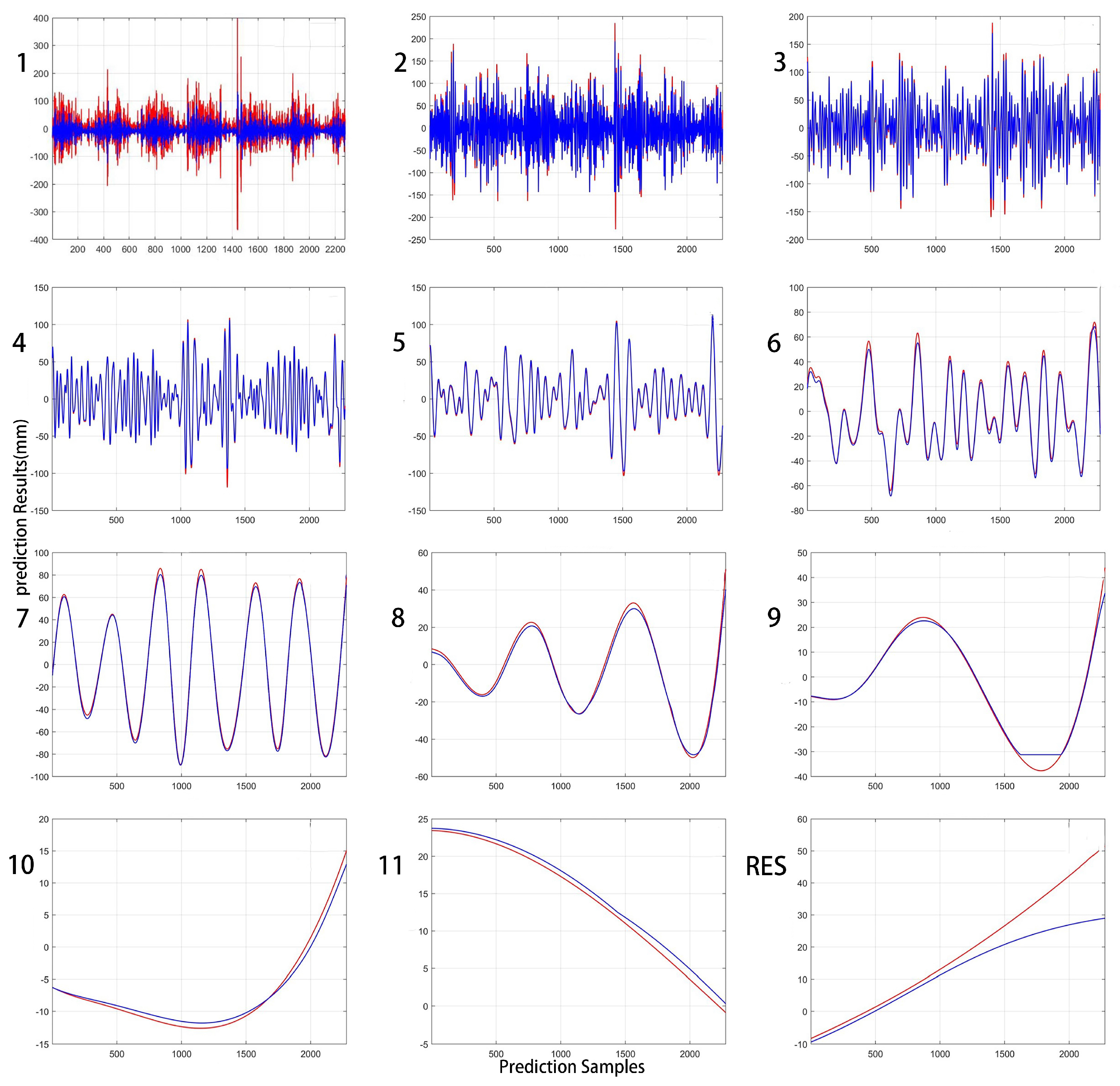
| RMSE | 46.37 | 10.09 | 4.98 | 1.89 | 2.38 | 3.54 | 2.65 | 2.06 | 2.17 | 0.84 | 0.88 | 8.48 |
| R2 | 0.26 | 0.96 | 0.99 | 0.99 | 0.99 | 0.99 | 0.99 | 0.99 | 0.99 | 0.99 | 0.97 | 0.76 |
| MAE | 30.40 | 7.28 | 3.98 | 1.25 | 2.13 | 2.94 | 2.39 | 1.68 | 1.29 | 0.82 | 1.28 | 5.84 |
| RMSE/mm | R2 | MAE/mm | |
|---|---|---|---|
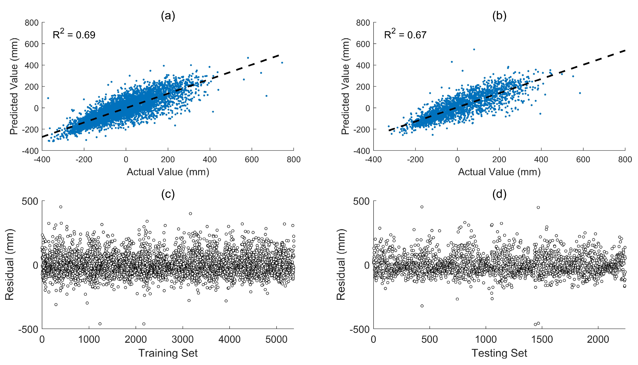
| LSTM-Training | 76.61 | 0.69 | 57.34 |
| LSTM-Testing | 81.06 | 0.67 | 59.22 |
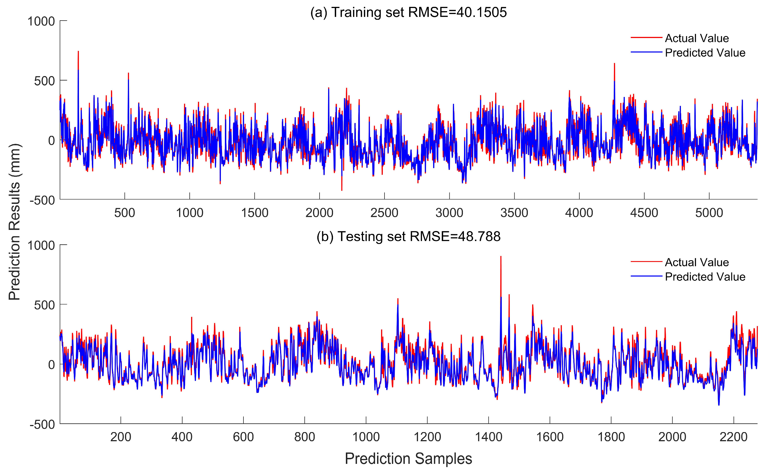
| EEMD-LSTM-Training | 40.15 | 0.91 | 28.74 |
| EEMD-LSTM-Testing | 48.79 | 0.88 | 34.21 |
Disclaimer/Publisher’s Note: The statements, opinions and data contained in all publications are solely those of the individual author(s) and contributor(s) and not of MDPI and/or the editor(s). MDPI and/or the editor(s) disclaim responsibility for any injury to people or property resulting from any ideas, methods, instructions or products referred to in the content. |
© 2023 by the authors. Licensee MDPI, Basel, Switzerland. This article is an open access article distributed under the terms and conditions of the Creative Commons Attribution (CC BY) license (https://creativecommons.org/licenses/by/4.0/).
Share and Cite
Yang, Y.; Cheng, Q.; Tsou, J.-Y.; Wong, K.-P.; Men, Y.; Zhang, Y. Multiscale Analysis and Prediction of Sea Level in the Northern South China Sea Based on Tide Gauge and Satellite Data. J. Mar. Sci. Eng. 2023, 11, 1203. https://doi.org/10.3390/jmse11061203
Yang Y, Cheng Q, Tsou J-Y, Wong K-P, Men Y, Zhang Y. Multiscale Analysis and Prediction of Sea Level in the Northern South China Sea Based on Tide Gauge and Satellite Data. Journal of Marine Science and Engineering. 2023; 11(6):1203. https://doi.org/10.3390/jmse11061203
Chicago/Turabian StyleYang, Yilin, Qiuming Cheng, Jin-Yeu Tsou, Ka-Po Wong, Yanzhuo Men, and Yuanzhi Zhang. 2023. "Multiscale Analysis and Prediction of Sea Level in the Northern South China Sea Based on Tide Gauge and Satellite Data" Journal of Marine Science and Engineering 11, no. 6: 1203. https://doi.org/10.3390/jmse11061203