Article

Theoretical Analysis Method for Roll Motion of Popup Data Communication Beacons

1
Institute of Deep-Sea Science and Engineering, Chinese Academy of Sciences, Sanya 572000, China
2
University of Chinese Academy of Sciences, Beijing 100049, China
*
Author to whom correspondence should be addressed.
J. Mar. Sci. Eng. 2023, 11(6), 1193; https://doi.org/10.3390/jmse11061193
Submission received: 23 April 2023 / Revised: 1 June 2023 / Accepted: 6 June 2023 / Published: 8 June 2023
(This article belongs to the Special Issue Young Researchers in Ocean Engineering)

Abstract

:
The popup data communication beacon (PDCB) can send data to the shore and ships through the BeiDou navigation satellite system (BDS) when it surfaces. The data can be collected by a deep-sea landing vehicle (DSLV) and transmitted using a magnetic induction coil. PDCBs can reduce the cost of DSLV recovery and redeployment. Whether the data can be successfully sent mainly depends on the outlet height and roll angle of the PDCB. Thus, accurately assessing the effect of the roll angle on data transmission is crucial. In this study, first, the differential equation of roll motion was preliminarily established using the small-amplitude wave theory along with the shape characteristics of the PDCB. Next, the nonlinear term of the recovery moment was processed using the Linz Ted Poincaré method. Then, the wave current force was analyzed using the Morrison theoretical formula along with an additional inertia moment calculation formula that is suitable for slender cylindrical small buoys. Finally, the theoretical calculation results were verified using the computational fluid dynamics (CFD) method and pool test. The roll angle error of the theoretical calculation was within 5%. Thus, the heave and roll response of PDCBs can be evaluated using theoretical calculation methods. The proposed calculation formula of additional inertia moment has guiding significance for the further optimization of the structure.

1. Introduction

With the extensive human exploration of the ocean, performing long-term, fixed-point observations of deep-sea areas are becoming increasingly necessary [1,2]. Traditional autonomous underwater vehicles (AUV) and remote underwater vehicles cannot accomplish this task [3,4]. Thus, deep-sea landing vehicles (DSLV) have attracted increased attention as underwater autonomous navigation platforms [5].
Due to the difficulty of deploying and maintaining instruments in the deep sea, the time cost of collecting deep-sea data and maintaining instruments is high [6]. The popup data communication beacon (PDCB) is an innovative solution for periodically sending data remotely. The data collected by the DSLV are transmitted using the magnetic induction coil which is placed at the bottom of the popup data communication beacon (PDCB) [7]. Data are stored on PDCB and once the collected data are sent to the base station through the BeiDou Navigation Satellite System (BDS) when it surfaces (Figure 1) [8,9]. This greatly reduces the time and cost of recycling and redeployment of DSLV.
DSLV is equipped with a variety of sensors such as a multiparameter water quality measurement instrument and RBR maestro [10], according to different requirements, as shown in Figure 2. Data are stored on the popup data communication beacon (PDCB) and once at the surface, and the measured data can be transmitted through satellites by releasing PDCBs.
The popup data communication beacon (PDCB) is a satellite communication buoy designed for release recovery by using DSLV. Whether the data can be successfully sent mainly depends on the height and roll angle of the PDCB above the sea surface. According to the structural design requirements of PDCB, the height of the PDCB above the water surface is 145 mm or more (including 110 mm of the BDS module). Thus, calculating the roll angle and evaluating its effect on data transmission are crucial [11,12].
The PDCB comprises an antenna chamber, a dome, a floating material, an electronic bay, and a magnetic induction coil, as shown in Figure 3. The pressure-resistant structure is made of a high-strength aluminum alloy, and the cap of the antenna cabin is made of polyether ether ketone (PEEK). The density of the floating material is 560 kg/m3. In practical applications, the dielectric constant and loss angle tangent of PEEK have little influence on the transmittance of radio waves [13]. In this study, a working depth of 4500 m was employed for PEEK; thus, meeting the requirements of pressure resistance, dimensional stability, corrosion resistance, aging resistance, and wave transmittance.
First, using the small-amplitude wave theory along with the shape characteristics of the PDCB to preliminarily establish the differential equation of the roll motion. Next, the Linzted Poincaré method is used to deal with the nonlinear term of the recovery moment. The dominant analysis of the wave current force was performed using the Morrison theoretical formula [14]. Moreover, the additional inertia moment calculation formula is proposed, which is suitable for slender cylindrical small floats. Furthermore, computational fluid dynamics (CFD) simulation based on STAR-CCM+ software and pool test were performed to demonstrate the feasibility of the theoretical calculation method. Data transmission results demonstrated that PDCBs can be used in the sea state with a Beaufort scale of 3, thus laying a foundation for further optimization of the structure.

2. Theoretical Calculations of the Roll Motion

In actual sea conditions, waves have relatively sharp peaks and relatively flat troughs. Stokes used mathematical equations to describe finite amplitude waves at the sea surface with relatively high accuracy [15,16,17]. However, these formulas are complex and difficult to apply directly in engineering practice.
All waves can be generated by superimposing numerous regular waves of different amplitudes and wavelengths, and regular waves [18], such as surges, are similar to plane waves in fluid mechanics. This makes it possible to study the motion performance of PDCBs when floating on the water surface through the motion performance of the plane wave.
According to fluid dynamics [19], the study of plane waves is based on the following assumptions:
(1)
The fluid is a non-viscous, incompressible ideal fluid.
(2)
The motion of fluid particles is a non-rotating potential flow motion.
(3)
The small-amplitude wave hypothesis is satisfied, that is, the wave height is small relative to the wavelength. The wave theory established according to this hypothesis is often referred to as the small-amplitude wave theory [20,21].

2.1. Sea State and Wave-Level Standards

Because no uniform wave-level standards have been established, to study the motion performance of PDCBs, we obtained the wave statistical characteristic data by using the Neumann spectrum formula:
S t ( ω ) = π c 2 ω 6 exp { 2 g 2 ω 2 U 2 } ,   ( m 2 · s ) ,
where c = 3.05   m 2 / s 5 , ω is the wave frequency ( s 1 ), g is the acceleration due to gravity ( 9.81   m / s 2 ), and U is the wind speed at 7.5 m above the sea surface ( m / s ).
The statistical characteristics of waves obtained using the Neumann spectrum formula are presented in Table 1 [22].

2.2. Establishment of Differential Equations for Roll Motion

The PDCB is a small-scale slender cylindrical marine structure used in the sea state with a Beaufort scale of 3 and an average wave height of 0.183 m. The diameter of the cylinder is 0.1 m, and the average wavelength of the sea surface ( λ ) is 6 m. Because D / λ < 0.1 , three assumptions must be made when analyzing the wave flow force [23]:
(1)
The changes in the surrounding flow field caused by the spatial distribution of the cylinder are ignored.
(2)
The flow field around cylindrical microelements are two-dimensional.
(3)
The direction of the wave flow force and the direction of movement of the cylinder are perpendicular to the axis.
Under the action of a single regular wave, the roll motion of the PDCB according to the small-amplitude wave theory, can be described using the second-order differential equation:
( J φ φ + Δ J φ φ ) φ ¨ + 2 N φ φ φ ˙ + F r ¯ φ = F a .
where J φ φ is moment of inertia; Δ J φ φ is additional moment of inertia; φ is roll angle; 2 N φ φ is damping factor; F is wave flow force; a  is the distance between the point of action of the resultant force of the wave flow force and the center of stability of the floating body.

2.2.1. Nonlinearity of the Recovery Moment

Compared with traditional communication buoys, the roll angle of small floats is large. Thus, the nonlinear components of the PDCB’s movement must be fully considered. However, the PDCB is a small-scale slender cylindrical marine structure and can be regarded as a weak nonlinear system. The nonlinear term in the recovery moment has a small value; thus, the solution of the nonlinear system can be obtained based on the linear system solution. The nonlinear factor is used as a perturbation of the linear system to perform an approximate analysis of the roll motion [24].
Linz et al. [25]. stated that the natural frequency n φ of a nonlinear system is not equal to the n φ 0 value of its derived system (a system that does not consider small parameters ε ) but is an unknown parameter that depends on ε . Therefore, when expanding the solution in the original system into a power series of ε , the natural frequency must be expanded into a power series of ε , and then the coefficients of the power series should be determined successively according to the requirements of periodic motion. The order should be determined according to the calculation accuracy requirements.
To simplify the derivation, the free vibration of the Duffin system is used as an example for the nonlinear analysis of the recovery moment [26]:
φ ¨ + n φ 0 2 ( φ + ε φ 3 ) = 0 .
The initial condition is set as
φ ( 0 ) = φ a ,   φ ˙ ( 0 ) = 0
The solution and the natural frequency of the original system are expanded into a power series of ε :
φ = φ 0 + ε φ 1 + ε 2 φ 2 + ,
n φ = n φ 0 + ε n φ 1 + ε 2 n φ 2 + ,
where n φ 0 is the natural frequency of the derived system. The square of both sides of the above formula is taken, and after arranging, we obtain
n φ 2 = n φ 0 2 ( 1 + ε σ 1 + ε 2 σ 2 + ) .
By substituting Equations (5) and (7) into Equation (3) and introducing a new independent variable ψ = n φ t , the original equation can be simplified by changing the differential sign to the original differential sign, that is, a differentiation of the ψ , such that each coefficient of the same power of the ε is zero, and the following approximate linear equations are obtained:
φ ¨ 0 + φ 0 = 0 ,
φ ¨ 1 + φ 1 = ( σ 1 φ ¨ 0 + φ 0 3 ) ,
φ ¨ 2 + φ 2 = ( σ 2 φ ¨ 0 + σ 1 φ ¨ 1 + 3 φ 0 2 φ 1 ) .
The initial conditions for each equation are as follows:
{ φ 0 ( 0 ) = φ a ,   φ ˙ 0 ( 0 ) = 0 φ 1 ( 0 ) = 0 ,   φ ˙ 1 ( 0 ) = 0 φ 2 ( 0 ) = 0 ,   φ ˙ 2 ( 0 ) = 0 .
Upon solving the zero-degree approximation equation (Equation (8a)) and the initial condition equation (Equation (9)), we obtain
φ 0 = φ a cos ψ .
Substituting this zero-degree approximation solution into the right-hand side of the approximation equation (Equation (8b)) and after simplification, we obtain
φ ¨ 1 + φ 1 = φ a ( σ 1 3 4 φ a 2 ) cos ψ 1 4 φ a 3 cos 3 ψ .
To ensure the periodicity of φ 1 ( t ) and avoid the duration term in the solution in Equation (11), the coefficient of cos ψ is considered zero. Accordingly, we obtain
σ 1 = 3 4 φ a 2 .
Substituting Equations (12) and (9) into Equation (11), we obtain
φ 1 = φ a 3 32 ( cos ψ cos 3 ψ ) .
Similarly, substituting Equation (10) into Equation (8c) gives the coefficient of cos ψ term as zero:
φ ¨ 2 + φ 2 = φ a ( σ 2 + 3 128 φ a 4 ) cos ψ + 24 128 φ a 5 cos 3 ψ 3 128 φ a 5 cos 5 ψ ,
σ 2 = 3 128 φ a 4 .
Substituting the initial condition (Equation (9)) into Equation (14) yields
φ 2 = φ a 5 1024 ( 23 cos ψ 24 cos 3 ψ + cos 5 ψ ) .
The above steps are repeated to obtain a periodic solution that satisfies the accuracy requirements:
φ = φ a cos ψ ε φ a 3 32 ( cos ψ cos 3 ψ ) + ε 2 φ a 5 1024 ( 23 cos ψ 24 cos 3 ψ + cos 5 ψ ) + = ( φ a ε φ a 3 32 + 23 ε 2 φ a 5 1024 + ) cos ψ + ( ε φ a 3 32 3 ε 2 φ a 5 128 + ) cos 3 ψ + .
Substituting σ 1 and σ 2 into Equation (7) yields
n φ 2 = n φ 0 2 ( 1 + 3 ε 4 φ a 2 3 ε 2 128 φ a 4 + ) .
where n φ is intrinsic frequency of nonlinear systems; n φ 0 is the inherent frequency of a linear system.
According to the accuracy requirements, the recovery moment F r ¯ φ can be expressed as follows:
F r ¯ φ = M h ( 1 + 3 ε 4 φ a 2 ) φ .

2.2.2. Determination of Wave Flow Force

Morison et al. proposed the Morrison theoretical formula [27], which states that the resultant force on slender structures in the ocean is composed of inertia force and drag force [28]. Comparing the relative importance of inertia force to drag force, the full Morrison theoretical formula can be simplified. The KC number is used by many marine engineers to perform the dominant analysis of inertia force and drag force [29,30], as shown in Table 2.
Keulegan and Carpenter studied the inertia force coefficient C M and drag force coefficient C D of slender cylinders and concluded that the dimensionless KC number can be expressed as
K C = u a T D ,
where u a is the amplitude of the flow rate (m/s), T is the period of the oscillating flow (s), and D is the diameter of the cylinder (m).
Because PDCBs are used in deep seas, the dispersion relationship must be used according to the situation of deep water waves, which can be obtained using the linear wave theory:
u = u a cos ( k x ω t ) ,
u a = ω A e k z ,
ω 2 = g k ,
where ω is the wave frequency (rad/s), A is the amplitude of the wave (m), k is the wavenumber ( m 1 ) , and z is the position of the cylinder.
The KC number of the PDCB when floating on the sea surface was calculated as 5.86. As can be observed from the contents of Table 2, the wave flow force is composed of an inertia force and a linearized drag force. The change of the spatial distribution of the surrounding flow field caused by the slender cylinder can be ignored. According to the Morrison theoretical formula, under the condition of waves and flows, the velocity field caused by the combination of wave flow, and object motion must be considered when calculating the drag force F D , and the incident wave force, disturbance wave force, and additional mass force F M generated by the motion of the floating body must be considered when calculating the inertia force. Thus, the wave flow force can be expressed as follows:
F = F M + F D ,
F M = 1 4 l ρ π D 2 C M V ˙ ( t ) 1 4 l ρ π D 2 C a X ¨ ( t ) ,
F D = 1 2 l ρ D C D ( V ( t ) + U X ˙ ( t ) ) | V ( t ) + U X ˙ ( t ) | .
According to Equations (20)–(22), Equation (11) can be expressed as
F M = 1 4 l ρ π D 2 [ C M ω 2 A e k z s i n ( k x ω t ) l C a φ ¨ ] .
Taking the waterline surface center of the PDCB as the origin, Equation (9) can be written as
F = 1 4 l ρ π D 2 [ C M ω 2 A e k z s i n ω t + l C a φ ¨ ] + 1 2 l ρ D C D ( V ( t ) + U X ˙ ( t ) ) | V ( t ) + U X ˙ ( t ) | .
where C D drag force factor; C M is inertial force coefficient; C a  is additional quality factor.

2.2.3. Nonlinearity of the Damping Moment

The damping force of the roll motion is positively correlated with the angular velocity. In the case of small-angle roll motion, the damping force can be considered proportional to the angular velocity. With the increase in the roll angle, the damping force gradually exhibits increasingly nonlinear characteristics. The PDCB is a small-scale slender cylindrical marine structure, and the damping ratio of the roll movement in the ocean is generally small (e.g., when the damping ratio is 0.1, the roll attenuation is considered to be very sharp). According to Equation (26), the drag force is the main cause of the nonlinear damping moment.

2.2.4. Correction of the Moment of Inertia

By simplifying the Morrison theoretical formula, additional torque during the roll motion can be obtained. The additional inertia moment is a function of the underwater part of the ocean float and depends on the shape of the object, direction of motion, acceleration, and other factors. In engineering applications, the additional inertia moment is generally calculated through model tests or empirical formulas, and theoretically, it is calculated using the slicing method or finite element method. By rearranging the F M terms in the inertial force of the Morrison theoretical formula, the additional inertia moment can be obtained; thus, the uncertainty of various parameters in the empirical formula can be avoided, and the complexity of theoretical calculations can be reduced.
According to Equation (25), the additional moment of inertia can be expressed as follows:
Δ J φ φ = π 4 a l 2 D 2 ρ C a .
By substituting Equations (5), (13), (15), and (16) into Equation (2), the theoretical calculation formula of roll motion can be obtained. The original roll differential equation comprehensively considers the additional moment of inertia, nonlinearity of the damping moment, and nonlinearity of the recovery moment when the small slender cylindrical float is at a large angle on the sea surface. The theoretical calculation formula is
( J φ φ + π 4 a l 2 D 2 ρ C a ) φ ¨ + 2 N φ φ φ ˙ + M h ( 1 + 3 ε 4 φ a 2 ) φ , = π 4 C M a A l D 2 ρ ω 2 e k z s i n ω t + 1 2 C D a l D ρ ( V ( t ) + U X ˙ ( t ) ) | V ( t ) + U X ˙ ( t ) | ,
where J φ φ is the moment of inertia, a is the distance between the resultant action point of the wave flow force and the center of stability of the floating body, l is the length of the floating body under water, D is the diameter of the floating body, ρ is the density of seawater, 2 N φ φ is the damping coefficient (twice the product of the damping ratio and natural frequency), C D is the drag force coefficient, C a is an additional quality factor, C M is the inertia force coefficient, ω is the wave frequency, A is the wave amplitude, k is the wavenumber, and z denotes the location being studied ( z = 0 represents the sea surface).

2.3. Analysis of Theoretical Calculation Results

According to Equation (30), the curve of the roll angle of a single regular wave acting on the PDCB can be plotted, as shown in Figure 4.
Under the synergistic effect of regular wave and constant flow, the PDCB changes to simple harmonic motion after a short irregular roll, with a period of approximately 2.5 s. The maximum roll angle of the simple harmonic motion is approximately 20°, and the equilibrium center of the motion is biased toward the direction of constant flow.
Drag force is the main source of the nonlinear damping moment. As the roll angle increases, the damping force gradually exhibits increasingly nonlinear characteristics. The PDCB is a small-scale slender cylindrical marine structure, and the damping ratio of floating body motion in the ocean is generally small. The analysis of the drag force term revealed that X ˙ ( t ) and | X ˙ ( t ) | are the main causes of the nonlinear damping moment.
The slender structure exhibits strong resistance to overturning. Although the center of the roll balance is always facing the direction of the constant flow, its posture can be quickly corrected when the angle is too large. In addition, the damping ratio of the buoy is generally small; thus, it can be considered that the period is similar to the inherent period. The period of the PDCB is approximately 2.5 s, which does not resonate with the waves, thus indicating high stability.

3. Simulation and Experimentation

3.1. Hydrodynamic Simulation

We established a simplified geometric model as shown in Figure 5. The head is a hemispherical cylindrical with a diameter of 100 mm, a total length of 871.9 mm, and a center-of-gravity height of 360 mm from the base.

3.1.1. Calculation Area

In CFD, the Gauss divergence theorem is used to convert differential equations such as N–S equations and k–ε equations into integral equations for calculations, and the integration region is a finite control body after the dispersion of the calculation domain. Thus, the calculation domain must be set reasonably. When setting the calculation domain, it must be ensured that the distance from the front end of the calculation object to the inlet is not less than 10 D (D is the diameter of the PDCB model), the distance from the back end of the calculation object to the outlet is not less than 15 D, and the interaction distance of the surrounding boundary is not less than 20 D.
Overlapping meshes and local encryption were used to create multiple compute domains outside of the buoy.
(1)
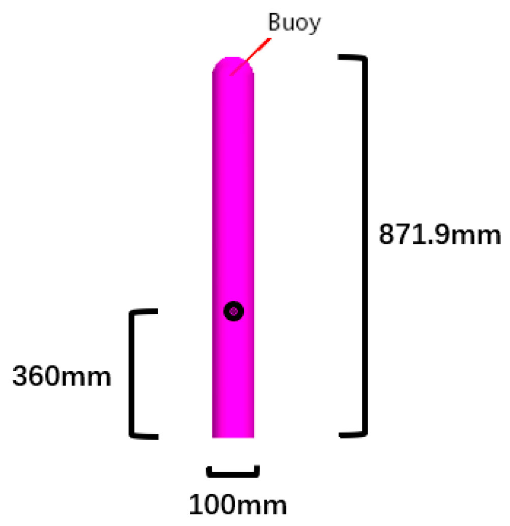
Background computational domain: The STAR-CCM+ simulation software automatically converts the wavelength to 9.03 m, while the PDCB has a diameter of 100 mm. PDCB is a small-scale object (λ/D ≈ 90 > 5), and its influence on the flow field is negligible. Thus, the x-direction, y-direction, and z-direction lengths of the background computational domain were set as 180 D, 50 D, and 50 D, respectively, and the center of mass of the PDCB model was located in the center of the computational domain to minimize the influence of the PDCB on the flow field of the background computational domain.
(2)
Background local encryption computational domain: The size of the background computational domain differs greatly from that of the PDCB. The local encryption method can avoid the problem of excessive calculation error and divergence; in addition, it can save computing resources. Therefore, the x-direction, y-direction, and z-direction lengths of the background local encryption computational domain were set as 20 D, 20 D of the diameter, and 3 m (approximately thrice the length of the PDCB), respectively. To reduce the difficulty of grid setup, the center of mass was located in the center of the computational domain.
(3)
Component grid computational domain: The overset grid is composed of the background grid and the component grid overlapping with each other. They overlap in space, but there is no connection relationship. As such, a connection relationship must be established through operations such as grid digging and interpolation. The overset grid area must be detailed in advance to provide a uniform, high-quality mesh that is otherwise prone to isolated cells. Therefore, the x-direction, y-direction, and z-direction lengths of this computational domain were set as 10 D, 10 D, and 2 m, respectively. The Boolean operation was used to accomplish the digging process.
(4)
Partial mesh local encryption computational domain: Setting this area can further improve the calculation accuracy of interactions. Thus, the x-direction, y-direction, and z-direction lengths of this computational domain were set as 10 D, 10 D, and 1.5 m, respectively.
(5)
Free-surface computational domain: This computational domain is used for the local refinement of the background domain mesh. The x-direction and y-direction lengths of the free-surface computational domain must be consistent with the background computational domain. Because the average wave height of the sea state is 0.183 m, the high z-plane of this computational domain was set as 0.187 m above the water surface, and the low z-plane was set as 0.212 m below the water surface. Setting the computational domain in this manner offers three advantages: the computational domain can cover two wave heights, the waterplane is approximately in the middle of this region, and the computational domain height is rounded off to facilitate grid division.

3.1.2. Mesh Model

(1)
Background grid settings: Set the base size as 1 m and the minimum size as 0.05 m, and the generated background mesh will automatically generate a mesh with a size between 0.05 m and 1 m according to the conditions. This setting can achieve the purpose of saving computing resources and is convenient to adapt to the free-surface mesh.
(2)
Background grid local encryption settings: By using the trimmer grid method, the grid was set as isotropic, and the absolute size was set as 0.1 m. The grid has an integer multiple relationship with the maximum absolute size of the background grid.
(3)
Partial grid settings: the surface mesh size was set as 0.005 m, which is equivalent to dividing the buoy into 20 grids along the diameter direction. The surface mesh has an integer multiple relationship with the background local encryption mesh, which facilitates data transmission. The overset mesh method requires high interpolation accuracy and requires the use of a double-precision solver. While the PDCB model is relatively simple, the use of a linear solver can greatly save computing resources while ensuring high accuracy.
(4)
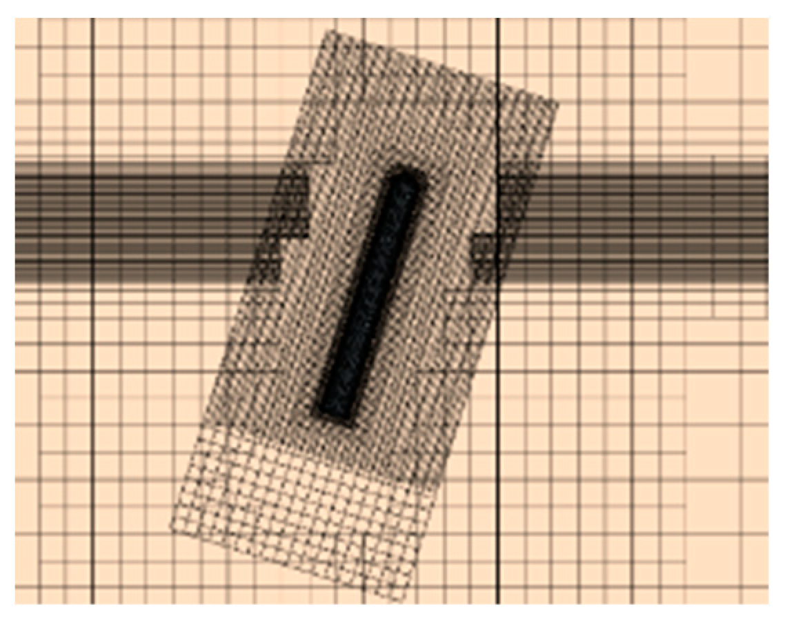
Partial mesh local encryption settings: The absolute x-direction and y-direction lengths were set as 0.005 m, which is consistent with the grid size of the surface of the PDCB. As can be seen in Figure 6, the grid size in the z-direction can be appropriately increased under the floating condition; thus, the absolute size of the grid in the z-direction was set as 0.02 m. Setting this area can further improve the computational accuracy of fluid–structure interactions. The local encryption grid exhibits a hierarchical relationship with the partial mesh, background local encryption grid, and background mesh, which aids in realizing data transmission and ensures the convergence of the calculation results. The local encryption grid and the free-surface grid exhibit an overlapping mesh relationship, which is conducive to the direct calculation of the interaction between the water surface wave and the PDCB.
(5)
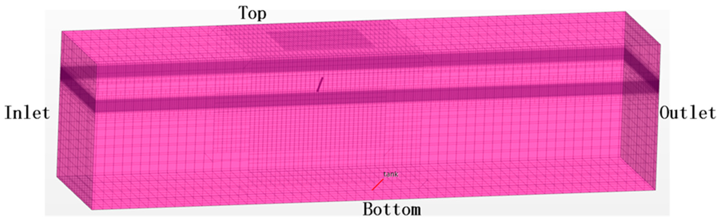
Free-surface mesh settings: Typically, 10–30 grids and 80–120 grids are set in the wave height direction and wavelength direction, respectively. The average wave height of the sea state is 0.183 m, and the average period is 2.4 s. STAR-CCM+ numerical simulation software can automatically convert the wavelength to 9.03 m. In this study, 18–19 grids were used to split the wave height and 90–91 grids were used to divide the wavelength so that each grid was 0.01 m in the wave height direction and 0.1 m in the wavelength direction, which aids in data transmission. The fluid domain length, width and height are 35 m × 8 m × 9 m.

3.1.3. Physical Model

The following physical models were selected: implicit unsteady, multiphase, volume of fluid (VOF), turbulent, k-epsilon turbulence, gravity, and VOF waves [31]. The shape and position of the free water surface were determined as shown in Figure 7.
The VOF algorithm is suitable for free-liquid surfaces as it can effectively deal with strong nonlinear phenomena such as the reconstruction of the free surface of the rising wave during the roll movement of the PDCB. As shown in Figure 7 and Figure 8, the algorithm can effectively construct and track the shape and position of the free surface according to the ratio function of the volume of heavy (seawater) and light fluids (air) in the grid cell.
Let F = 0 represent that the grid is filled with air and F = 1 represent that the grid is full of seawater. By using the six-degrees-of-freedom motion model and the k-epsilon turbulence model, the floating motion of the PDCB can be simulated. The F-function satisfies the following equation:
F t + u F x + v F y + ω F z = 0 .
The setting of the time step needs to be calculated according to the following formula, and the actual selected time step is less than the calculated time step.
Δ t S T A R = W a v e   P e r i o d N u m b e r   o f   C e l l s   p e r   W a v e   L e n g t h   ×   2.4 ( 2 π T ) 2 = g 2 π λ t a n h ( 2 π λ   d )
where T is the wave period; g is the acceleration of gravity, take 9.81 m / s 2 ; λ is the wavelength, take 6 m; d is the water depth, take 10 m. Calculate T ≈ 2 s, since the number of grids for each wavelength is 60, so the calculated Δ t S T A R = 0.0144 s, the actual selected time step is 0.001 s.
The overlapping grid method was used to simulate the roll motion process till 50 s. The roll angle result obtained through simulation is shown in Figure 9. The roll angle tended to be regular from 20 s onwards, where the maximum roll angle was approximately 21°, and the average value was approximately 20°. The equilibrium center direction coincided with the direction of constant flow. The error between the simulated roll angle and the calculated roll angle was less than 5%. The period was approximately 2.5 s, which is the same as that obtained through theoretical calculations.

3.2. Simulation Results and Pool Test

After the PDCB was released, it floated up to the water’s surface. Then, it made a roll motion with a wave height of approximately 0.183 m. An attitude sensor with a sampling frequency of 1 s was installed inside the electronic cabin to monitor the real-time roll angle of the buoy, as shown in Figure 10. To determine whether the buoy can communicate normally, it is checked whether the BDS module is transmitting data to the receiver. If the data is received, it indicates that the communication is good while performing roll angle measurements.
The pool test is shown in Figure 10 and Figure 11. After the PDCB surfaced for the first time, the outlet height under the action of inertia was very high; thus, the first swing angle was the largest (33°). Subsequently, its outlet height rapidly reduced until it stabilized at around 145 mm, thus satisfying the requirements of normal communication outlet height, and the roll amplitude decreased rapidly. The results show that the data transmitted back by the attitude sensor can be received, which demonstrates effective communication.
The error between the roll angle obtained using the CFD simulation and the roll angle calculated theoretically was less than 5%. The period was approximately 2.5 s, as shown in the Figure 12, which is the same as that obtained through theoretical calculations.

4. Discussion

In this paper, we presented the expression for additional inertia for small floating bodies, facilitating the calculation of roll motion. The traditional method of calculating the additional inertia is often based on the ship type or large buoy and is difficult to directly apply to a small float. In contrast, the additional inertia derived using the Morrison theoretical formula fully considers the geometric characteristics of the slender cylinder; thus, it is highly suitable for PDCBs.
At present, only the single degree of freedom traverse is considered and more simplifications have been made, the uncertainty of the drag coefficient is large, and the selection of many parameters in the additional moment of inertia depends on experience. In addition, the study of theoretical calculation methods, especially the use of Linz Ted—Poincaré’s method, is based on small-angle rollover motion. Subsequently, the theoretical calculation method when the roll angle is large under the harsh sea state can be studied.
In the CFD simulation process, the application of overlapping mesh and local encryption can greatly save computing resources while ensuring calculation accuracy. On the one hand, the local encryption grid forms a hierarchical relationship with the component grid, the background local encryption grid and the background grid, which realizes the step-by-step transmission of data and ensures the convergence of the calculation results, on the other hand, the local encryption grid and the free surface mesh form an overlapping grid relationship, which is conducive to the more direct calculation of the interaction between water surface waves and PDCB, and further improves the calculation accuracy of interaction. The simulation of the roll motion of PDCB when floating on the sea surface is of great significance to whether the structural design of PDCB meets the needs for use.

5. Conclusions

(1)
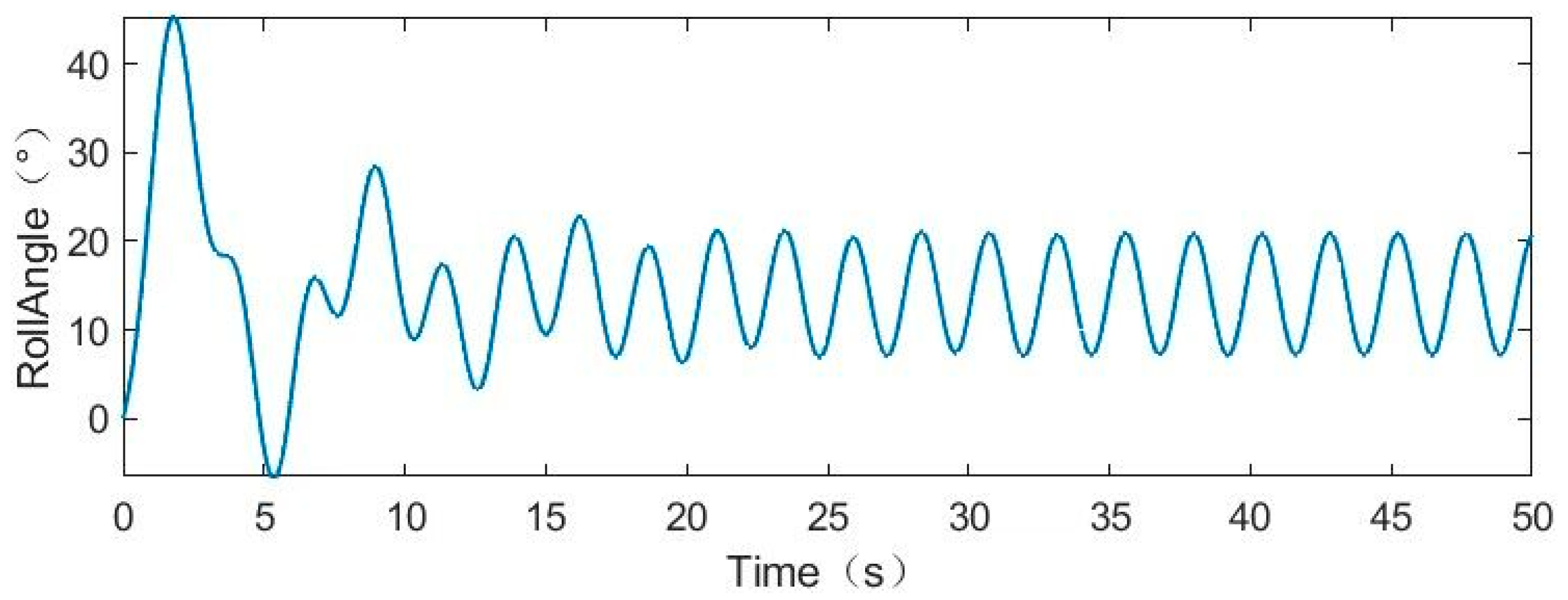
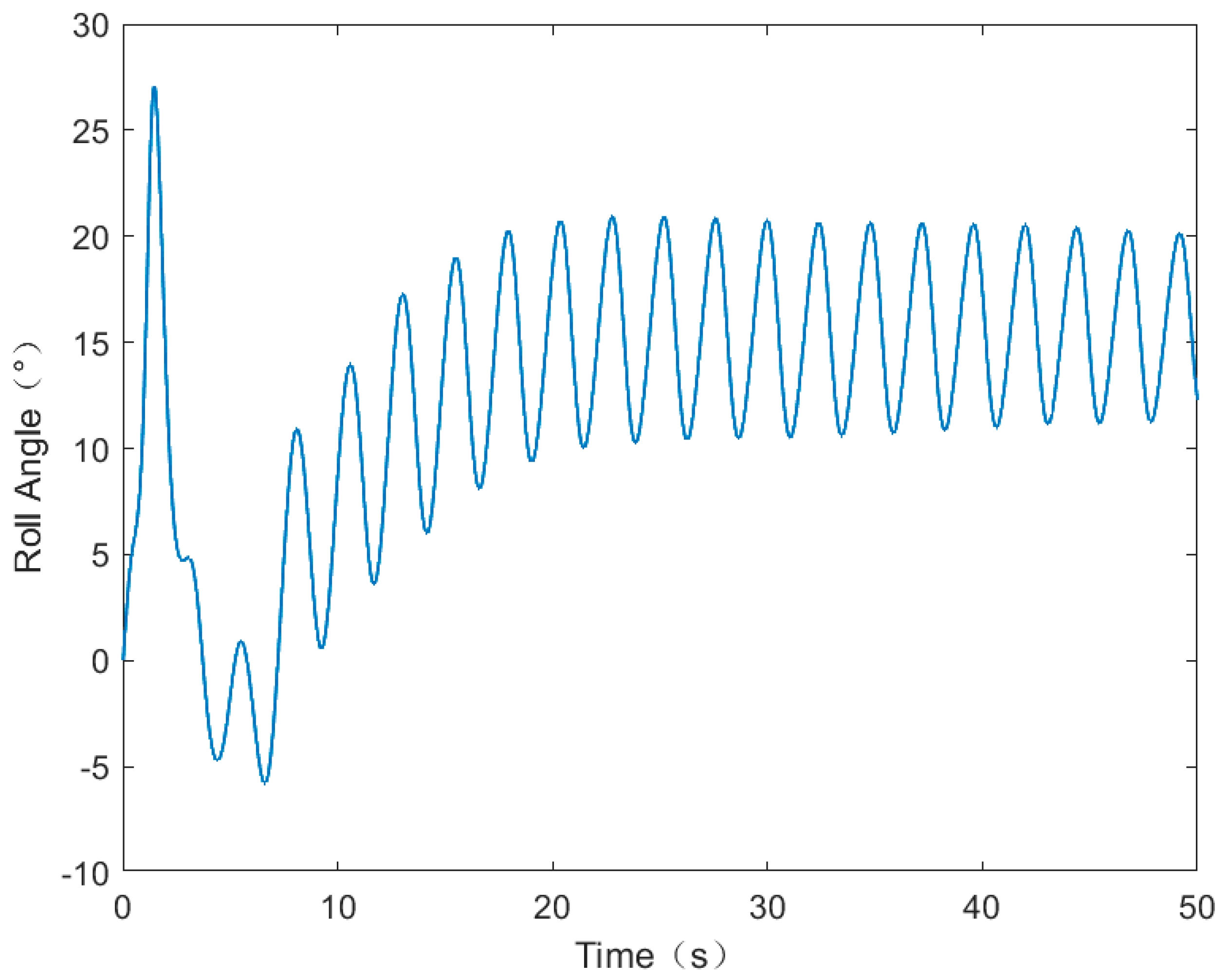
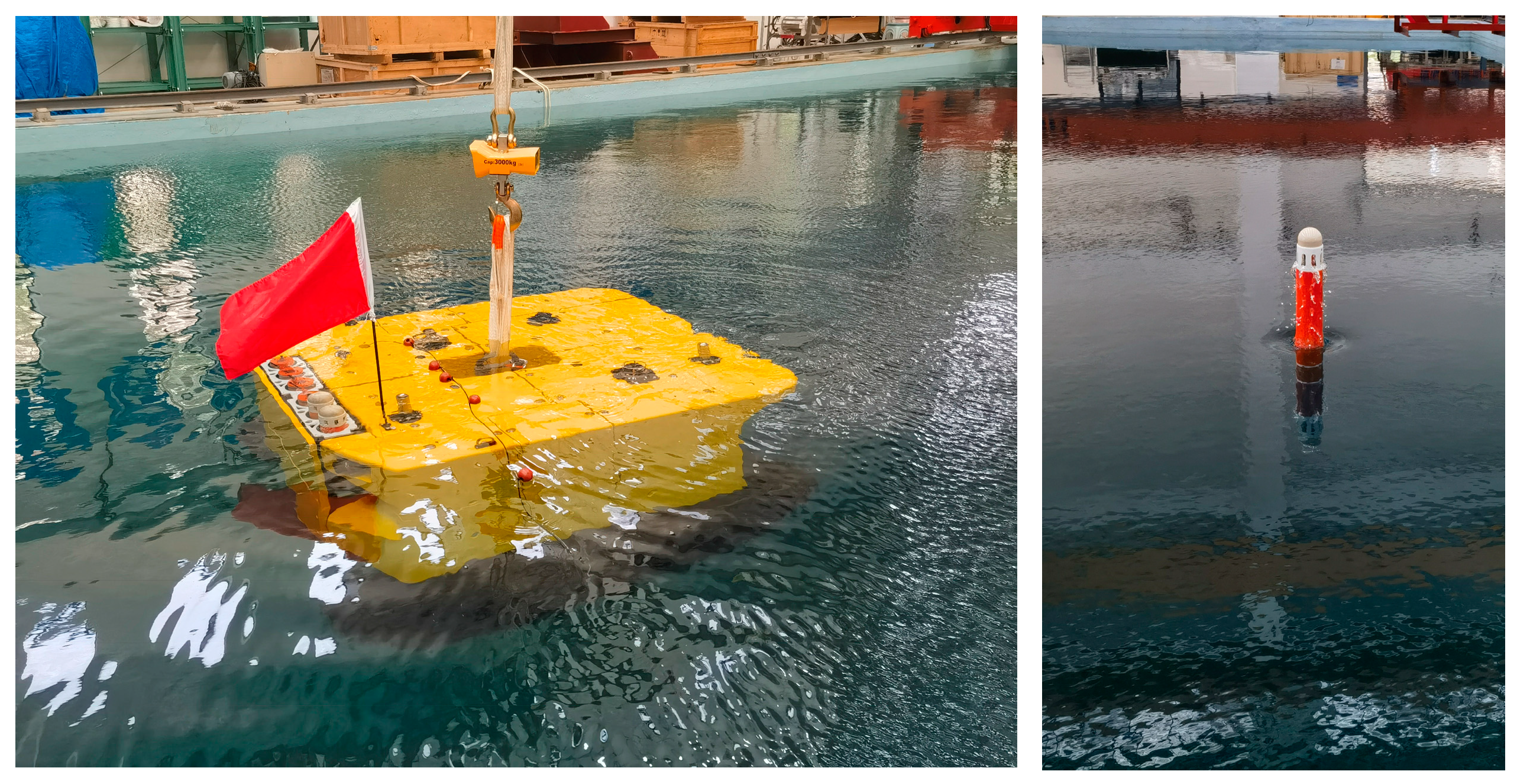
The design of PDCBs can be accomplished using the theoretical calculation method to meet the communication requirements. The comparison of the hydrodynamic simulation and pool test, the maximum roll angle error calculated theoretically is less than 5%, and the roll period is similar (~2.5 s). By using the theoretical calculation method, the roll motion can be predicted, and resonance between the floating body and the wave can be avoided during the design process.
(2)
We reduced the difficulty of processing nonlinear terms. We introduced the Morrison theoretical formula in the differential equation of roll motion and analyzed the inertia force and drag force by using the KC number. The Morrison theoretical formula fully considers the characteristics of the floating slender cylinder. In contrast, the processing of the nonlinear term by using the Linz Ted Poincaré method can appropriately omit the higher harmonics according to the accuracy requirements, simplifying the equation of roll motion. The processing method of the differential equation of roll motion proposed in this paper has guiding significance for the structural design, motion prediction, improvement, and optimization of small buoys.
(3)
We presented a clear expression for calculating the additional inertia for small buoys, which facilitates the calculation of roll motion. Traditional methods of calculating the additional inertia are often based on ship types or large buoys and are difficult to apply directly to small buoys. The additional inertia obtained using the Morrison theoretical formula fully considers the characteristics of slender cylindrical small floats; thus, it is highly suitable for PDCBs and has guiding significance for the structural design of other types of small floats.

Author Contributions

Conceptualization, C.T.; methodology, C.T. and Y.S.; software, H.C.; writing—original draft preparation, Y.S. and H.C.; writing—review and editing, Y.S. and L.Y.; visualization, Y.S., H.C., and C.W.; supervision, C.T.; project administration, C.T.; funding acquisition, C.T. All authors have read and agreed to the published version of the manuscript.

Funding

This research was funded by The Major Scientific and Technological Projects of Hainan Province, grant numbers ZDKJ202016.

Institutional Review Board Statement

Not applicable.

Informed Consent Statement

Not applicable.

Data Availability Statement

The data presented in this study are available in this article (Tables and Figures).

Acknowledgments

We thank Shiliu Peng for their help in revising the wording of this paper. We also thank the Institute of Deep-Sea Science and Engineering, Chinese Academy of Sciences for providing hydrostatic pressure testing and sea trial opportunity.

Conflicts of Interest

The authors declare no conflict of interest.

Abbreviations

The following abbreviations are used in this manuscript:
PDCBThe Popup Data Communication Beacon
DSLVDeep-Sea Landing Vehicle
AUVAutonomous Underwater Vehicle
BDSBeiDou navigation satellite System
VOFVolume of Fluid
CFDComputational Fluid Dynamics)

References

  1. Weller, R.A.; Baker, D.J.; Glackin, M.M.; Roberts, S.J.; Schmitt, R.W.; Twigg, E.S.; Vimont, D.J. The Challenge of Sustaining Ocean Observations. Front. Mar. Sci. 2019, 6, 105. [Google Scholar] [CrossRef]
  2. Venkatesan, R.; Tandon, A.; Sengupta, D.; Navaneeth, K. Recent Trends in Ocean Observations. In Observing the Oceans in Real Time; Springer: Cham, Switzerland, 2018; pp. 3–13. [Google Scholar]
  3. Matsuda, T.; Takizawa, R.; Sakamaki, T.; Maki, T. Landing method of autonomous underwater vehicles for seafloor surveying. Appl. Ocean Res. 2020, 101, 102221. [Google Scholar] [CrossRef]
  4. Griffiths, G. Technology and Applications of Autonomous Underwater Vehicles; CRC Press: Boca Raton, FL, USA, 2002; Volume 2. [Google Scholar]
  5. Sun, H.; Guo, W.; Lan, Y.; Wei, Z.; Gao, S.; Sun, Y.; Fu, Y. Black-Box Modelling and Prediction of Deep-Sea Landing Vehicles Based on Optimised Support Vector Regression. J. Mar. Sci. Eng. 2022, 10, 575. [Google Scholar] [CrossRef]
  6. Garzoli, S.; Boebel, O.; Bryden, H.; Fine, R.A.; Fukasawa, M.; Gladyshev, S.; Johnson, G.; Johnson, M.; MacDonald, A.; Meinen, C. Progressing towards global sustained deep ocean observations. In Proceedings of the OceanObs’09, Venice-Lido, Italy, 21–25 September 2009. [Google Scholar]
  7. Karstensen, J.; Motz, M.; Hansen, B.; Larsen, K.; Rayner, D. Technical Enhancement of TMA Sites for Data Safety & Cost Efficiency; AtlantOS: Kiel, Germany, 2018. [Google Scholar]
  8. Liu, Q.; Chen, Y. Research on sea surface drifting buoy based on Beidou communication System. In Proceedings of the 2017 5th International Conference on Frontiers of Manufacturing Science and Measuring Technology (FMSMT 2017), Taiyuan, China, 24–25 June 2017; pp. 1300–1304. [Google Scholar]
  9. Luo, P.; Song, Y.; Xu, X.; Wang, C.; Zhang, S.; Shu, Y.; Ma, Y.; Shen, C.; Tian, C. Efficient Underwater Sensor Data Recovery Method for Real-Time Communication Subsurface Mooring System. J. Mar. Sci. Eng. 2022, 10, 1491. [Google Scholar] [CrossRef]
  10. Halverson, M.; Jackson, J.; Richards, C.; Melling, H.; Brunsting, R.; Dempsey, M.; Gatien, G.; Hamilton, A.; Hunt, B.; Jacob, W. Guidelines for Processing RBR CTD Profiles; Fisheries and Oceans Canada= Pêches et océans Canada: Ottawa, ON, Canada, 2017. [Google Scholar]
  11. Sugimura, D.; Arai, M.; Sakaguchi, K.; Araki, K.; Sotoyama, T. A study on beam tilt angle of base station antennas for base station cooperation systems. In Proceedings of the 2011 IEEE 22nd International Symposium on Personal, Indoor and Mobile Radio Communications, Toronto, ON, Canada, 11–14 September 2011; pp. 2374–2378. [Google Scholar]
  12. Ling, C.; Yin, X.; He, Y.; Ruiz Boqué, S. Attitude Estimation for In-Service Base Station Antenna Using Downlink Channel Fading Statistics. Int. J. Antennas Propag. 2015, 2015, 898631. [Google Scholar] [CrossRef] [Green Version]
  13. Xia, X.; Zhang, H.; Lu, T.; Gulliver, T.A. Design of a beidou satellite radome for deep-sea buoys. In Proceedings of the 2017 IEEE Pacific Rim Conference on Communications, Computers and Signal Processing (PACRIM), Victoria, BC, Canada, 21–23 August 2017; pp. 1–5. [Google Scholar]
  14. Zan, X.; Lin, Z.; Gou, Y. The Force Exerted by Surface Wave on Cylinder and Its Parameterization: Morison Equation Revisited. J. Mar. Sci. Eng. 2022, 10, 702. [Google Scholar] [CrossRef]
  15. Tsuji, Y.; Nagata, Y. Stokes’ expansion of internal deep water waves to the fifth order. J. Oceanogr. Soc. Jpn. 1973, 29, 61–69. [Google Scholar] [CrossRef]
  16. Fenton, J.D. A fifth-order Stokes theory for steady waves. J. Waterw. Port Coast. Ocean Eng. 1985, 111, 216–234. [Google Scholar] [CrossRef] [Green Version]
  17. Karambas, T.V.; Koutitas, C.G. An improvement to Stokes nonlinear theory for steady waves. J. Waterw. Port Coast. Ocean Eng. 1998, 124, 36–39. [Google Scholar] [CrossRef]
  18. Chen, L.F.; Zang, J.; Hillis, A.J.; Morgan, G.C.J.; Plummer, A.R. Numerical investigation of wave–structure interaction using OpenFOAM. Ocean Eng. 2014, 88, 91–109. [Google Scholar] [CrossRef] [Green Version]
  19. Zank, G.P.; Matthaeus, W.H. The equations of nearly incompressible fluids. I. Hydrodynamics, turbulence, and waves. Phys. Fluids A Fluid Dyn. 1991, 3, 69–82. [Google Scholar] [CrossRef]
  20. Ursell, F.; Dean, R.G.; Yu, Y.S. Forced small-amplitude water waves: A comparison of theory and experiment. J. Fluid Mech. 2006, 7, 33–52. [Google Scholar] [CrossRef]
  21. Choun, Y.-S.; Yun, C.-B. Sloshing analysis of rectangular tanks with a submerged structure by using small-amplitude water wave theory. Earthq. Eng. Struct. Dyn. 1999, 28, 763–783. [Google Scholar] [CrossRef]
  22. Pierson, W.J. Practical Methods for Observing and Forecasting Ocean Waves by Means of Wave Spectra and Statistics; Hydrographic Office: Washington, DC, USA, 1958. [Google Scholar]
  23. Paidoussis, M.P. Flow-induced Instabilities of Cylindrical Structures. Appl. Mech. Rev. 1987, 40, 163–175. [Google Scholar] [CrossRef]
  24. Merchant, H.; Kelf, M. Nonlinear analysis of submerged ocean buoy systems. In Proceedings of the Ocean 73-IEEE International Conference on Engineering in the Ocean Environment, Seattle, WA, USA, 25–28 September 1973; pp. 390–395. [Google Scholar]
  25. Verhulst, F.; Verhulst, F. The Poincaré-Lindstedt method. In Nonlinear Differential Equations and Dynamical Systems; Springer: Berlin/Heidelberg, Germany, 1996; pp. 122–135. [Google Scholar]
  26. Nedjadi, Y.; Barrett, R. The Duffin-Kemmer-Petiau oscillator. J. Phys. A Math. Gen. 1994, 27, 4301. [Google Scholar] [CrossRef] [Green Version]
  27. Morison, J.; Johnson, J.W.; Schaaf, S.A. The force exerted by surface waves on piles. J. Pet. Technol. 1950, 2, 149–154. [Google Scholar] [CrossRef]
  28. Sumer, B.M. Hydrodynamics around Cylindrical Strucures; World Scientific: Singapore, 2006; Volume 26. [Google Scholar]
  29. Cotter, D.C.; Chakrabarti, S.K. Wave force tests on vertical and inclined cylinders. J. Waterw. Port Coast. Ocean Eng. 1984, 110, 1–14. [Google Scholar] [CrossRef]
  30. Keulegan, G.H.; Carpenter, L.H. Forces on Cylinders and Plates in an Oscillating Fluid; U.S. Department of Commerce National Bureau of Standards: Washington, DC, USA, 1956. [Google Scholar]
  31. Lu, Y.; Shao, W.; Gu, Z.; Wu, C.; Li, C. Research on ship motion characteristics in a cross sea based on computational fluid dynamics and potential flow theory. Eng. Appl. Comput. Fluid Mech. 2023, 17, 2164618. [Google Scholar] [CrossRef]
Figure 1. Data transmission.
Jmse 11 01193 g001
Figure 2. RBR maestro.
Jmse 11 01193 g002
Figure 3. Structure of the PDCB.
Jmse 11 01193 g003
Figure 4. Roll curve obtained using the theoretical calculation method.
Jmse 11 01193 g004
Figure 5. Geometric model.
Jmse 11 01193 g005
Figure 6. Partial mesh local encryption settings.
Jmse 11 01193 g006
Figure 7. The computational domain and the boundaries (Perspective View).
Jmse 11 01193 g007
Figure 8. The shape and position of the free water surface.
Jmse 11 01193 g008
Figure 9. Roll monitor plot obtained using the computational fluid dynamics method.
Jmse 11 01193 g009
Figure 10. Attitude sensor.
Jmse 11 01193 g010
Figure 11. Pool test of the PDCB.
Jmse 11 01193 g011
Figure 12. Theoretical calculation of roll angle of PDCB under the influence of waves, CFD simulation, and comparison of experimental measurement results.
Jmse 11 01193 g012
Table 1. Wave characteristic data.
Beaufort ScaleWind Velocity (m/s) h ¯
(m)
h 1 / 3  
(m)
The Period of the Wave (s)Wavelength (m)
RangeAverageRangeAverage
00~0.2000000
10.3~1.50.0150.020~1.00.50~0.90.10
21.6~3.30.0550.090.4~2.81.40.7~252.00
33.4~5.40.1830.300.8~4.92.42~606.00
45.5~7.90.5490.881.6~7.63.98~11616.00
58.0~10.71.3112.102.8~10.65.415~19331.00
610.8~13.82.5004.003.8~13.67.024~30050.00
713.9~17.14.4507.004.8~17.08.737~44078.00
817.2~20.77.01011.306.0~20.510.551~610115.00
Table 2. Dominant analysis of drag force and inertial force.
KC Number.Dominance Analysis
KC < 3The inertia force accounts for the main component.
3 < KC < 15Inertia force + linearized drag force.
15 < KC < 45Inertia force + complete nonlinear drag force.
KC > 45The drag force accounts for the main component.
Disclaimer/Publisher’s Note: The statements, opinions and data contained in all publications are solely those of the individual author(s) and contributor(s) and not of MDPI and/or the editor(s). MDPI and/or the editor(s) disclaim responsibility for any injury to people or property resulting from any ideas, methods, instructions or products referred to in the content.

