
A Side-Scan Sonar Image Synthesis Method Based on a Diffusion Model

Abstract
:1. Introduction
2. Methods
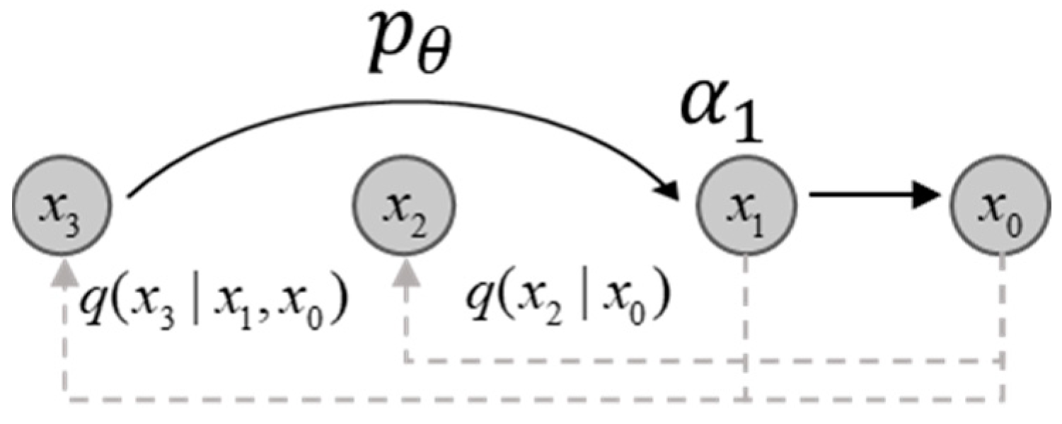
2.1. Diffusion Mode
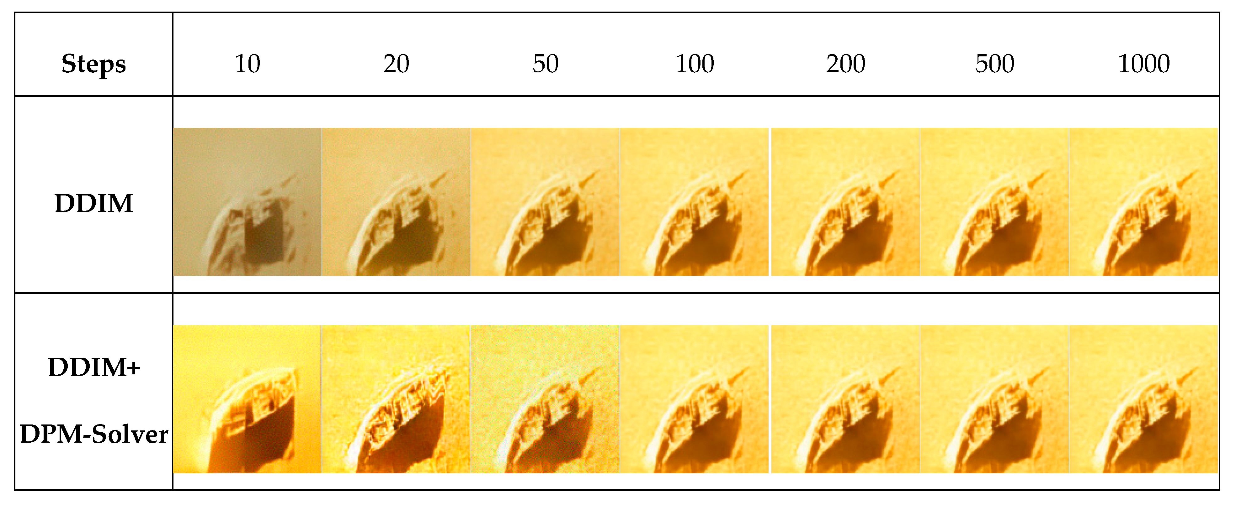
2.2. DPM-Solver
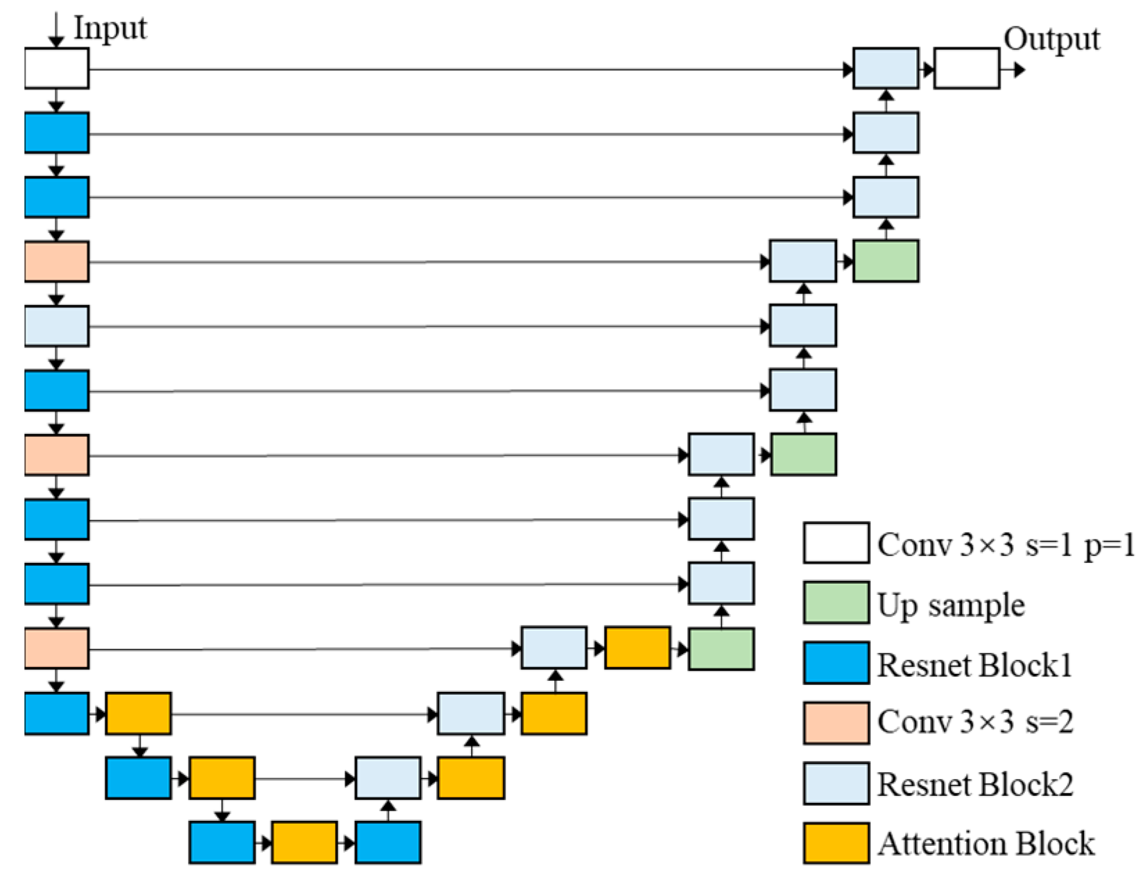
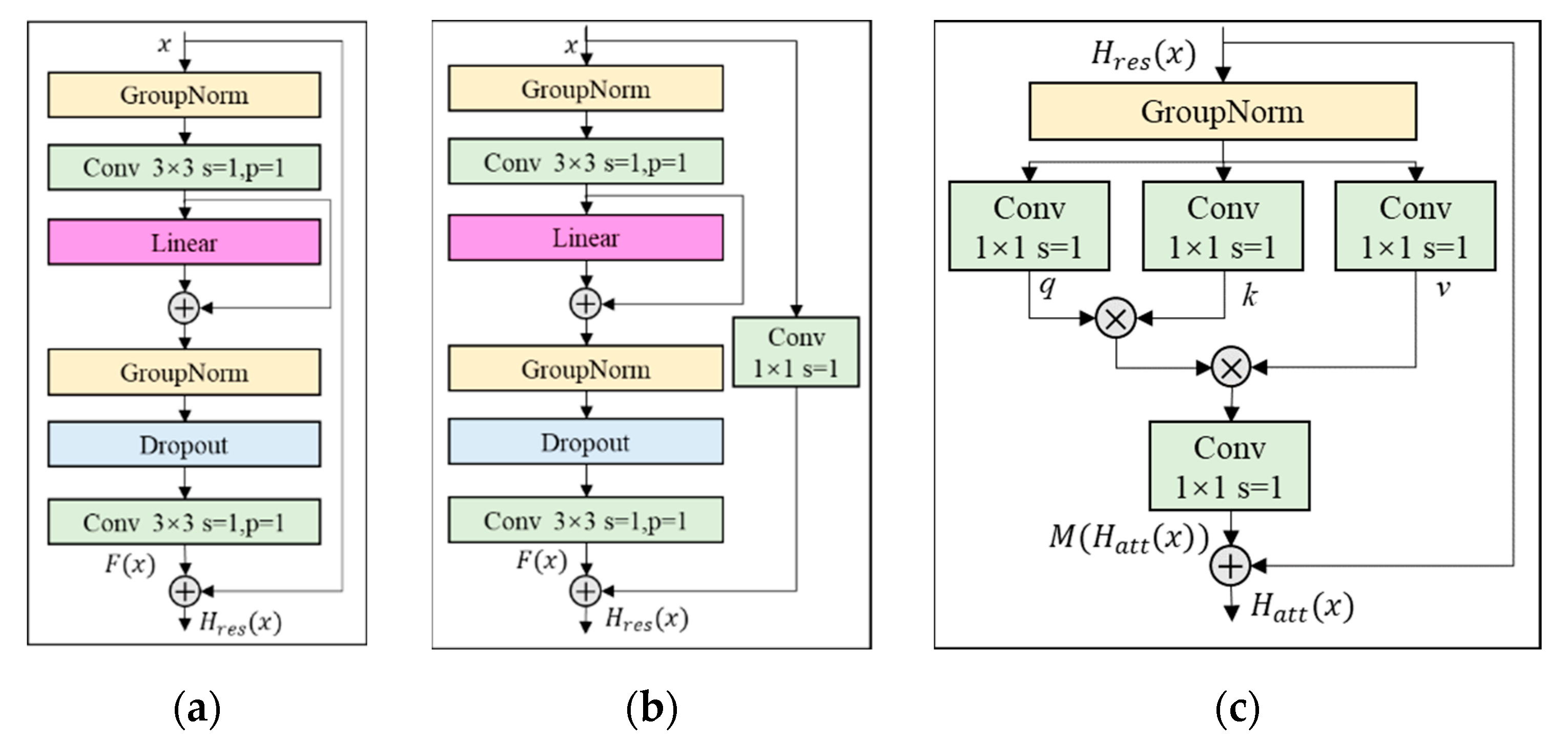
2.3. Model Structure
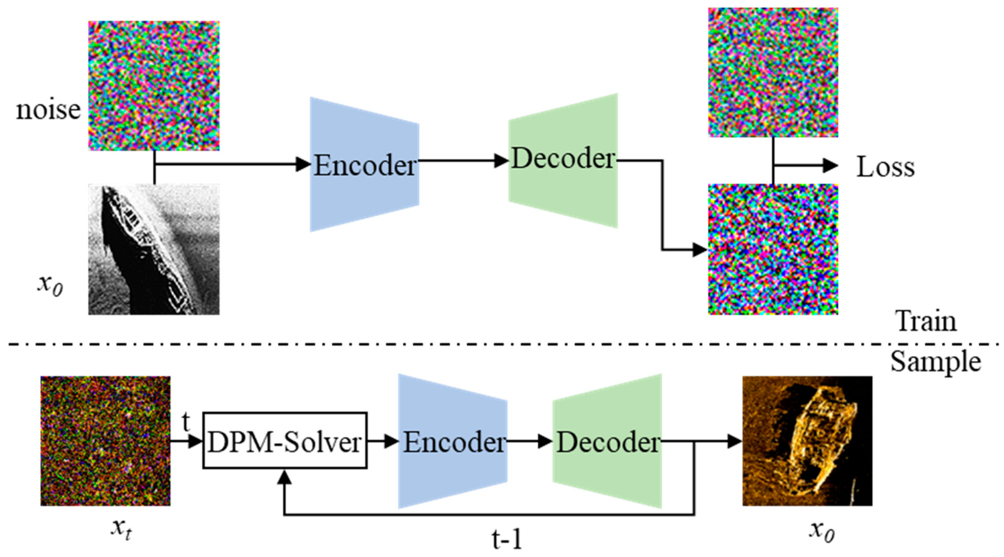
2.4. Model Training and Sample Generation Process
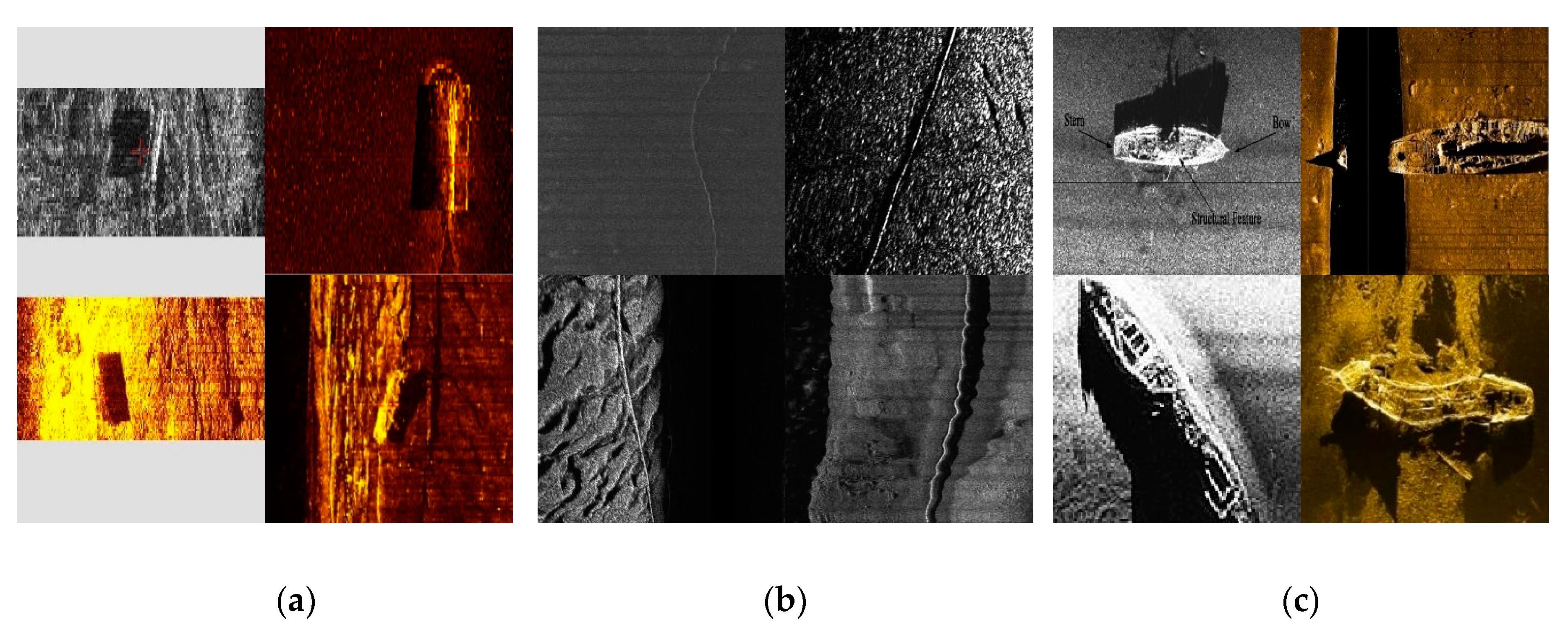
3. Experimental Validation
3.1. Evaluation Metrics
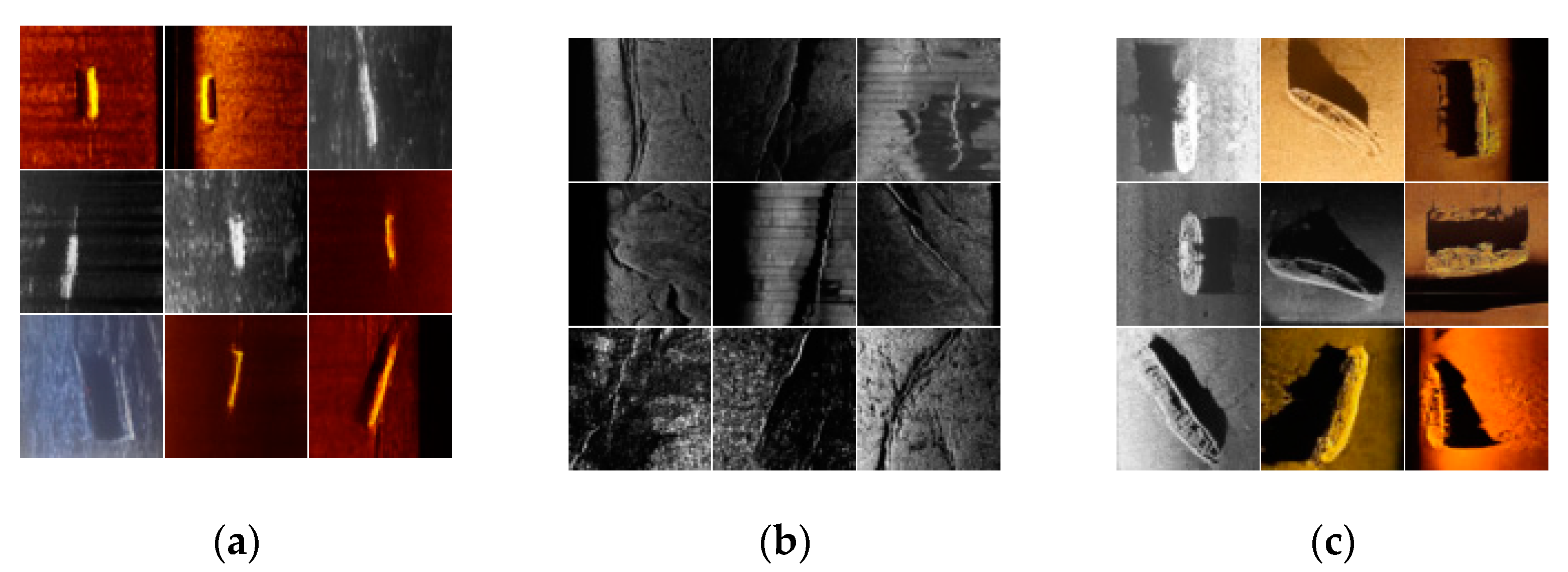
3.2. Experimental Design and Image Generation
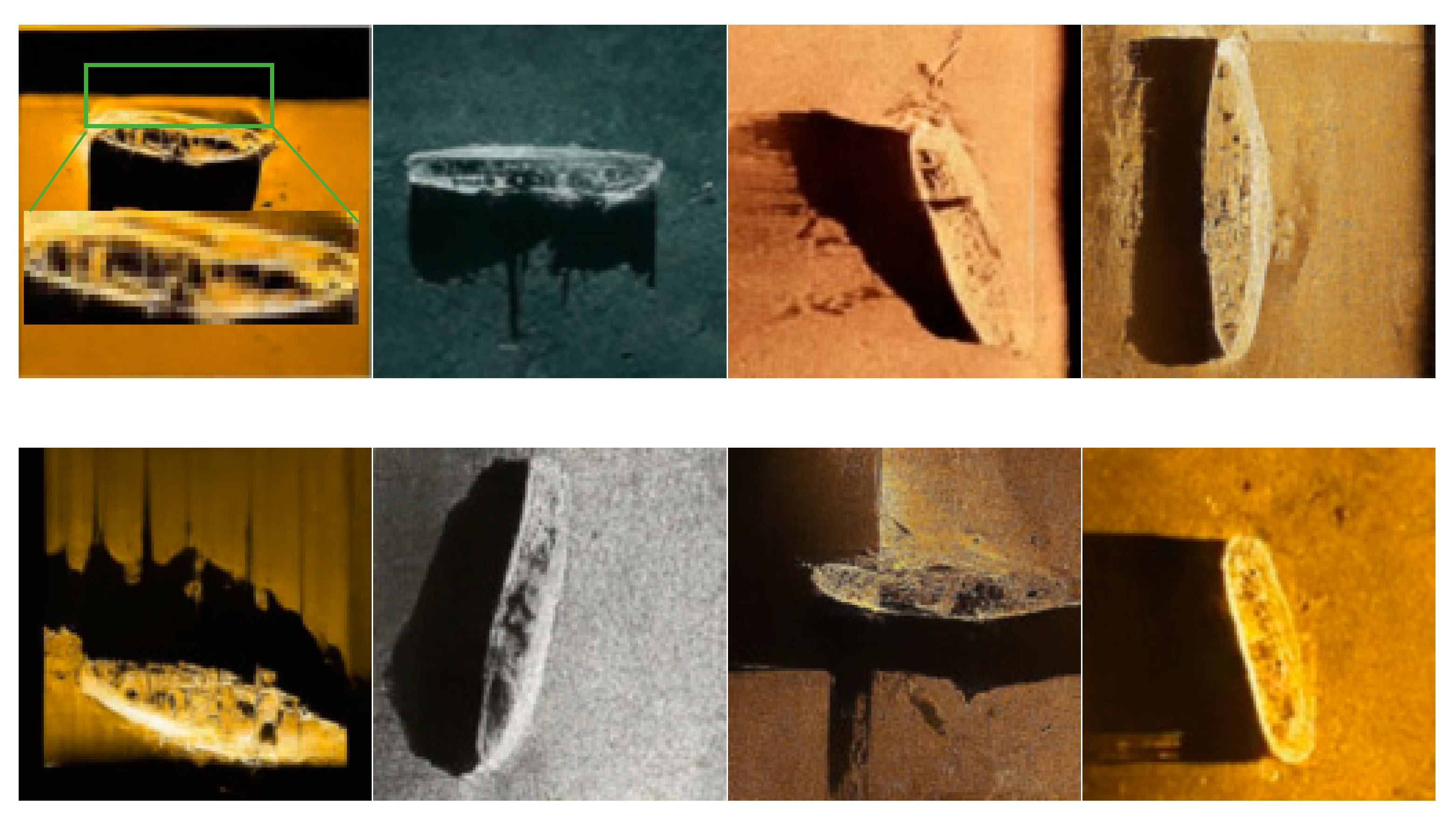
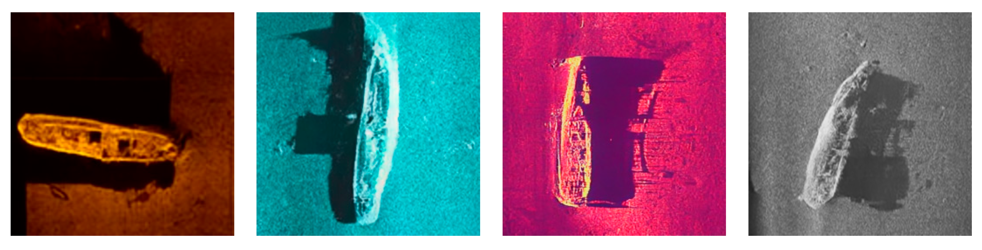
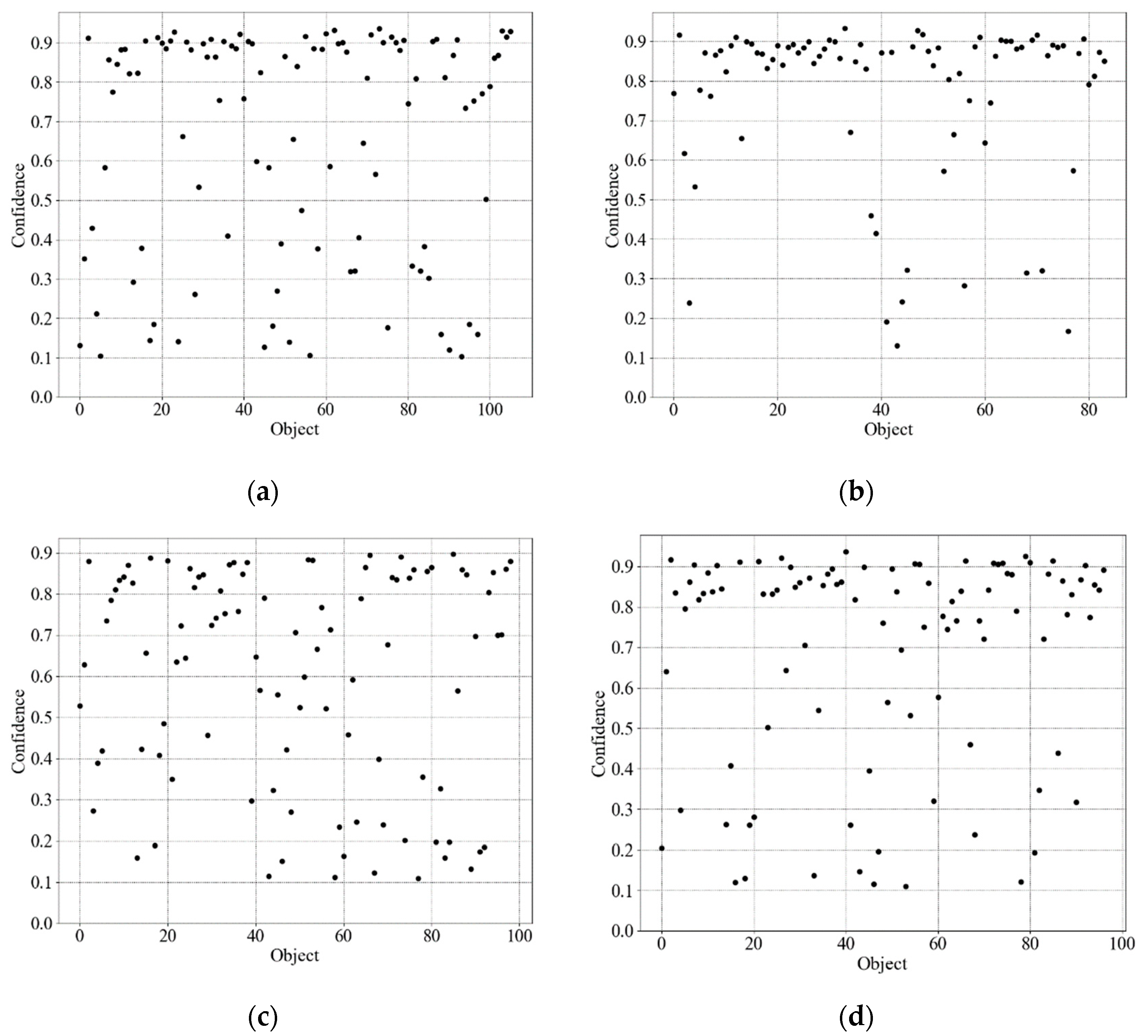
3.3. Qualitative Analysis
3.4. Wreck Object Detection Model Training
4. Discussion
4.1. Difference between Different Sampling Steps
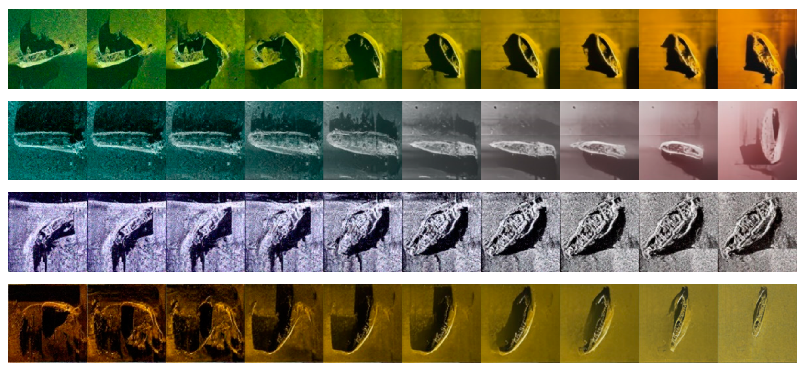
4.2. Effect of Different Noise Inputs on Sample Generation
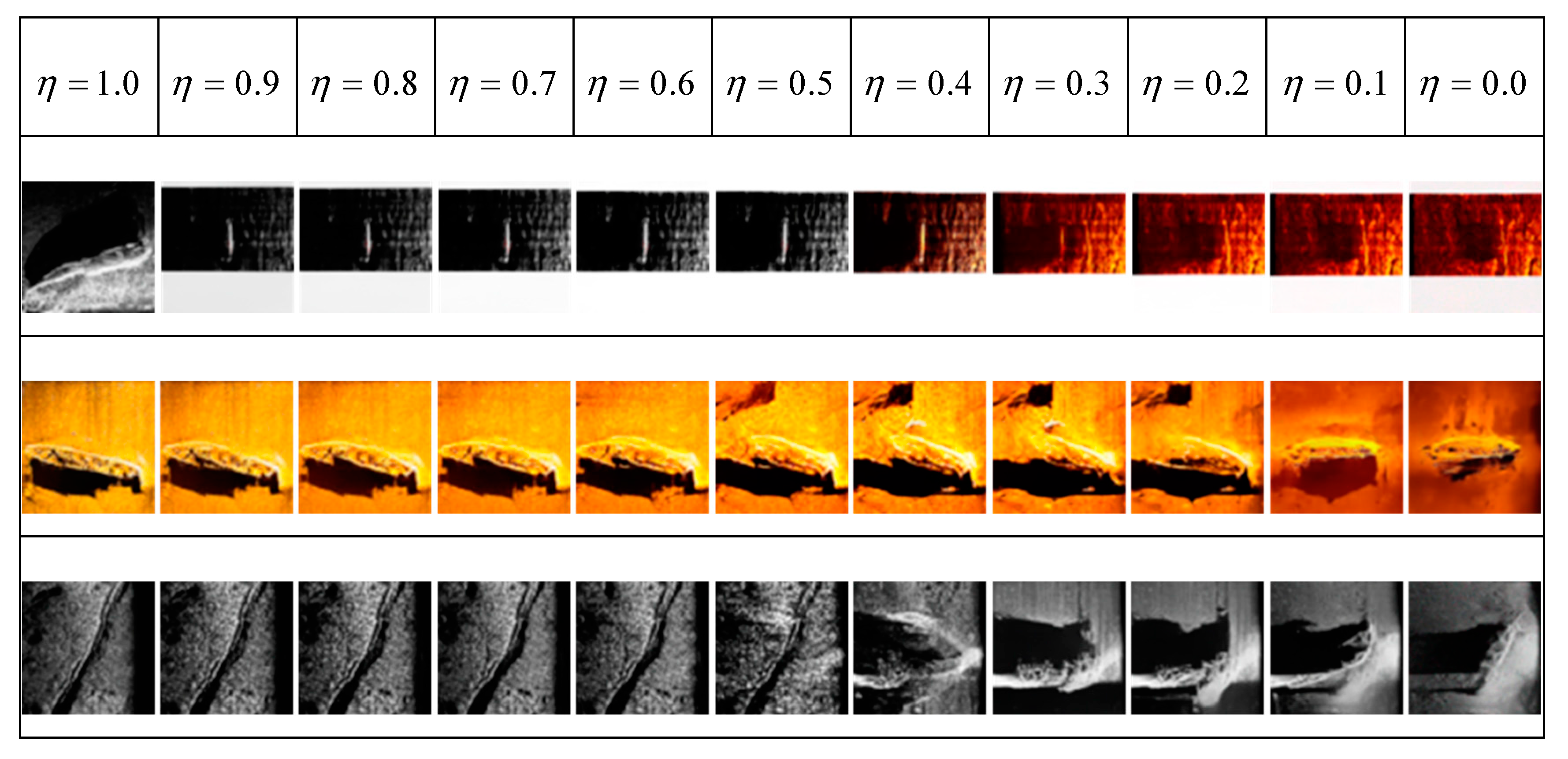
4.3. The Effect of Random Noise on Sample Generation
5. Conclusions
Author Contributions
Funding
Data Availability Statement
Acknowledgments
Conflicts of Interest
References
- Yu, Y.; Zhao, J.; Gong, Q.; Huang, C.; Zheng, G.; Ma, J. Real-time underwater maritime object detection in side-scan sonar images based on transformer-YOLOv5. Remote Sens. 2021, 13, 3555. [Google Scholar] [CrossRef]
- Cvikel, D.; Grøn, O.; Boldreel, L.O. Detecting the Ma’agan Mikhael B shipwreck. Underw. Technol. 2016, 34, 93–98. [Google Scholar] [CrossRef]
- Xiaonan, C.; Minyan, L.; Longjun, H. Shipwreck statistical analysis and suggestions for ships carrying liquefiable solid bulk cargoes in China. Proc. Eng. 2014, 84, 188–194. [Google Scholar] [CrossRef]
- Piccinelli, M.; Gubian, P. Modern ships voyage data recorders: A forensics perspective on the Costa concordia shipwreck. Digit. Investig. 2013, 10, 41–49. [Google Scholar] [CrossRef]
- Ødegård, Ø.; Mogstad, A.A.; Johnsen, G.; Sørensen, A.J.; Ludvigsen, M. Underwater hyperspectral imaging: A new tool for marine archaeology. Appl. Opt. 2018, 57, 3214–3223. [Google Scholar] [CrossRef]
- Greene, A.; Rahman, A.F.; Kline, R.; Rahman, M.S. Side scan sonar: A cost-efficient alternative method for measuring seagrass cover in shallow environments. Estuar. Coast. Shelf Sci. 2018, 207, 250–258. [Google Scholar] [CrossRef]
- Girshick, R.; Donahue, J.; Darrell, T.; Malik, J. Region-based convolutional networks for accurate object detection and semantic segmentation. IEEE Trans. Pattern Anal. Mach. Intell. 2016, 38, 142–158. [Google Scholar] [CrossRef]
- Tan, C.; Sun, F.; Kong, T.; Zhang, W.; Yang, C.; Liu, C. A survey on deep transfer learning. In Proceedings of the Artificial Neural Networks and Machine Learning-ICANN 2018: 27th International Conference on Artificial Neural Networks, Rhodes, Greece, 4–7 October 2018; pp. 270–279. [Google Scholar]
- Nayak, N.; Nara, M.; Gambin, T.; Wood, Z.; Clark, C.M. Machine learning techniques for AUV side-scan sonar data feature extraction as applied to intelligent search for underwater archaeological sites. Field Serv. Robot. 2021, 16, 219–233. [Google Scholar]
- Nguyen, H.-T.; Lee, E.-H.; Lee, S. Study on the classification performance of underwater sonar image classification based on convolutional neural networks for detecting a submerged human body. Sensors 2019, 20, 94. [Google Scholar] [CrossRef]
- Lee, S.; Park, B.; Kim, A. Deep learning from shallow dives: Sonar image generation and training for underwater object detection. arXiv 2018, arXiv:1810.07990. [Google Scholar]
- Huo, G.; Wu, Z.; Li, J. Underwater object classification in sidescan sonar images using deep transfer learning and semisynthetic training data. IEEE Access 2020, 8, 47407–47418. [Google Scholar] [CrossRef]
- Ge, Q.; Ruan, F.; Qiao, B.; Zhang, Q.; Zuo, X.; Dang, L. Side-scan sonar image classification based on style transfer and pre-trained convolutional neural networks. Electronics 2021, 10, 1823. [Google Scholar] [CrossRef]
- Li, C.; Ye, X.; Cao, D.; Hou, J.; Yang, H. Zero shot objects classification method of side scan sonar image based on synthesis of pseudo samples. Appl. Acoust. 2021, 173, 107691. [Google Scholar] [CrossRef]
- Huang, C.; Zhao, J.; Yu, Y.; Zhang, H. Comprehensive Sample Augmentation by Fully Considering SSS Imaging Mechanism and Environment for Shipwreck Detection Under Zero Real Samples. IEEE Trans. Geosci. Remote Sens. 2021, 60, 1–14. [Google Scholar] [CrossRef]
- Karras, T.; Laine, S.; Aittala, M.; Hellsten, J.; Lehtinen, J.; Aila, T. Analyzing and improving the image quality of stylegan. In Proceedings of the IEEE/CVF Conference on Computer Vision and Pattern Recognition, Seattle, WA, USA, 14–19 June 2020; pp. 8110–8119. [Google Scholar]
- van den Oord, A.; Dieleman, S.; Zen, H.; Simonyan, K.; Vinyals, O.; Graves, A.; Kalchbrenner, N.; Senior, A.; Ka-vuk-cuoglu, K. WaveNet: A generative model for raw audio. arXiv 2016, arXiv:1609.03499. [Google Scholar]
- Goodfellow, I.; Pouget-Abadie, J.; Mirza, M.; Xu, B.; Warde-Farley, D.; Ozair, S.; Courville, A.; Bengio, Y. Generative Adversarial Nets in Advances in Neural Information Processing Systems (NIPS); Curran Associates, Inc.: Red Hook, NY, USA, 2014; pp. 2672–2680. [Google Scholar]
- van den Oord, A.; Kalchbrenner, N.; Kavukcuoglu, K. Pixel recurrent neural networks. arXiv 2016, arXiv:1601.06759. [Google Scholar]
- Rezende, D.J.; Mohamed, S. Variational inference with normalizing flows. arXiv 2015, arXiv:1505.05770. [Google Scholar]
- Kingma, D.P.; Welling, M. Auto-Encoding variational bayes. arXiv 2013, arXiv:1312.6114v10. [Google Scholar]
- Bore, N.; Folkesson, J. Modeling and Simulation of Side scan Using Conditional Generative Adversarial Network. IEEE J. Ocean. Eng. 2021, 46, 195–205. [Google Scholar] [CrossRef]
- Jiang, Y.F.; Ku, B.; Kim, W.; Ko, H. Side-Scan Sonar Image Synthesis Based on Generative Adversarial Network for Im-ages in Multiple Frequencies. IEEE Geosci. Remote Sens. Lett. 2021, 18, 1505–1509. [Google Scholar] [CrossRef]
- Brock, A.; Donahue, J.; Simonyan, K. Large scale GAN training for high fidelity natural image synthesis. arXiv 2018, arXiv:1809.11096. [Google Scholar]
- Karras, T.; Laine, S.; Aila, T. A Style-Based generator architecture for generative adversarial networks. arXiv 2018, arXiv:1812.04948. [Google Scholar]
- Sohl-Dickstein, J.; Weiss, E.; Maheswaranathan, N.; Ganguli, S. Deep unsupervised learning using nonequilibrium ther-modynamics. In Proceedings of the International Conference on Machine Learning, Lille, France, 6–11 July 2015; pp. 2256–2265. [Google Scholar]
- Ho, J.; Jain, A.; Abbeel, P. Denoising diffusion probabilistic models. arXiv 2020, arXiv:2006.11239. [Google Scholar]
- Song, J.; Meng, C.; Ermon, S. Denoising diffusion implicit models. arXiv 2020, arXiv:2010.02502. [Google Scholar]
- Lu, C.; Zhou, Y.; Bao, F.; Chen, J.; Li, C.; Zhu, J. DPM-Solver: A Fast ODE Solver for Diffusion Probabilistic Model Sam-pling in Around 10 Steps. arXiv 2022, arXiv:2206.00927. [Google Scholar]
- Atkinson, K.; Han, W.; Stewart, D.E. Numerical Solution of Ordinary Differential Equations; John Wiley & Sons: Hoboken, NJ, USA, 2011; Volume 108. [Google Scholar]
- Hochbruck, M.; Ostermann, A. Exponential integrators. Acta Numer. 2010, 19, 209–286. [Google Scholar] [CrossRef]
- Ronneberger, O.; Fischer, P.; Brox, T. U-net: Convolutional networks for biomedical image segmentation. In Proceedings of the Medical Image Computing and Computer-Assisted Intervention–MICCAI 2015: 18th International Conference, Munich, Germany, 5–9 October 2015; Proceedings, Part III 18. Springer International Publishing: Berlin/Heidelberg, Germany, 2015; pp. 234–241. [Google Scholar]
- Xiao, X.; Lian, S.; Luo, Z.; Li, S. Weighted res-unet for high-quality retina vessel segmentation. In Proceedings of the2018 9th International Conference on Information Technology in Medicine and Education (ITME), Hangzhou, China, 19–21 October 2018; pp. 327–331. [Google Scholar]
- He, K.; Zhang, X.; Ren, S.; Sun, J. Deep residual learning for image recognition. In Proceedings of the IEEE Conference on Computer Vision and Pattern Recognition, Las Vegas, NV, USA, 27–30 June 2016; pp. 770–778. [Google Scholar]


| Group | Training Set Category | Batch Size | Image Size |
|---|---|---|---|
| T1 | Shipwreck, Container, Pipeline | 40 | 64 × 64 |
| T2 | Shipwreck | 11 | 128 × 128 |
| T3 | Shipwreck | 3 | 256 × 256 |
| Model | Target | FID | MMD | PSNR | SSIM | LPIPS |
|---|---|---|---|---|---|---|
| T1 | Shipwreck | 138.56 | 0.2357 | 11.1764 | 0.1753 | 0.3942 |
| Container | 108.869 | 0.2324 | 10.0542 | 0.2512 | 0.426 | |
| Pipeline | 102.656 | 0.2343 | 15.1054 | 0.208 | 0.2921 | |
| T2 | Shipwreck | 153.59 | 0.1194 | 10.6517 | 0.1769 | 0.4415 |
| T3 | Shipwreck | 153.75 | 0.0601 | 10.3241 | 0.18114 | 0.4969 |
| Group | Training Set | Number | Test Set | Number |
|---|---|---|---|---|
| G1 | SSS Images | 205 | SSS Images | 81 |
| G2 | Generate images (128 × 128/256 × 256) | 8765 | SSS Images | 81 |
| G3 | Generate image (128 × 128) | 5794 | SSS Images | 81 |
| G4 | Generate image (256 × 256) | 2971 | SSS Images | 81 |
| Group | Training Set | Prediction | Recall |
|---|---|---|---|
| G1 | SSS Images | 0.888 | 0.84 |
| G2 | Generate images (128 × 128/256 × 256) | 0.93 | 0.851 |
| G3 | Generate image (128 × 128) | 0.929 | 0.702 |
| G4 | Generate image (256 × 256) | 0.922 | 0.755 |
Disclaimer/Publisher’s Note: The statements, opinions and data contained in all publications are solely those of the individual author(s) and contributor(s) and not of MDPI and/or the editor(s). MDPI and/or the editor(s) disclaim responsibility for any injury to people or property resulting from any ideas, methods, instructions or products referred to in the content. |
© 2023 by the authors. Licensee MDPI, Basel, Switzerland. This article is an open access article distributed under the terms and conditions of the Creative Commons Attribution (CC BY) license (https://creativecommons.org/licenses/by/4.0/).
Share and Cite
Yang, Z.; Zhao, J.; Zhang, H.; Yu, Y.; Huang, C. A Side-Scan Sonar Image Synthesis Method Based on a Diffusion Model. J. Mar. Sci. Eng. 2023, 11, 1103. https://doi.org/10.3390/jmse11061103
Yang Z, Zhao J, Zhang H, Yu Y, Huang C. A Side-Scan Sonar Image Synthesis Method Based on a Diffusion Model. Journal of Marine Science and Engineering. 2023; 11(6):1103. https://doi.org/10.3390/jmse11061103
Chicago/Turabian StyleYang, Zhiwei, Jianhu Zhao, Hongmei Zhang, Yongcan Yu, and Chao Huang. 2023. "A Side-Scan Sonar Image Synthesis Method Based on a Diffusion Model" Journal of Marine Science and Engineering 11, no. 6: 1103. https://doi.org/10.3390/jmse11061103