Article

Hydrokinetic Power Potential in Spanish Coasts Using a Novel Turbine Design

by
Mahmoud I. Ibrahim
1,2 and
María José Legaz
3,*
1
Department of Naval Architecture and Marine Engineering, Faculty of Engineering, Alexandria University, Alexandria 21544, Egypt
2
Laboratório de Sistemas e Tecnologia Subaquática (LSTS), Faculdade de Engenharia, Universidade do Porto, 4200-465 Porto, Portugal
3
Department of Applied Physics and Naval Technology, Faculty of Naval and Ocean Engineering, Technical University of Cartagena, 30203 Cartagena, Spain
*
Author to whom correspondence should be addressed.
J. Mar. Sci. Eng. 2023, 11(5), 942; https://doi.org/10.3390/jmse11050942
Submission received: 27 March 2023 / Revised: 26 April 2023 / Accepted: 26 April 2023 / Published: 28 April 2023
(This article belongs to the Special Issue Tidal and Wave Energy)

Abstract

:
Nowadays, there is great concern about obtaining clean energy. Governments around the world are boosting renewable energy resources. Oceans provide abundant renewable energy resources, including tidal, wave, and current energy. It seems that ocean currents are one of the most promising ways to obtain energy from the oceans. The goal of this paper is to assess the hydrokinetic power potential in three different areas of the Spanish coast using a novel turbine design, named the fin-ring turbine. The patented turbine was previously power tested in 2014 in the Gulf of Mexico and numerically validated in the literature. A three-dimensional computational fluid dynamics (CFD) simulation of the novel current turbine is presented, including mesh sensitivity and turbulence studies. The turbine’s performance represented in TSR-Cp is discussed. The turbine was simulated in different regions with several current speeds, focusing on the Spanish coast. The results are very promising, with upper limit power coefficients of 37.5%, and 36.5% as a lower limit. Also, the comparisons with power test data available in the literature show very satisfactory agreement. The results highlight the superiority of the turbine in lower currents and present the suitability of the turbine’s applicability.

1. Introduction

According to [1], energy demand is going to grow by approximately 37% by 2040. In addition to this, fossil fuel reserves are decreasing [2], and governments around the world are worried about the effects of global warming and climate change [3]. All of this has led to great interest in exploiting renewable energy resources. Not only have oceans and seas played a significant role in the growth of human civilization, but they can also be key players in the provision of clean, limitless energy. Ocean energy resources have the potential to provide approximately 120,000 TWh/year [4], which could be enough to produce more than 400% of the current global demand for electricity. This enormous potential is partially linked to the huge variety of extraction principles, including wave, tidal, marine current, ocean thermal, and osmotic (salinity gradient) techniques [4].
One of the most promising among them is undoubtedly linked to ocean currents. Wind is what typically drives ocean surface currents. However, tides, river discharge, pressure gradients (created, for example, by sea-surface slopes built up by coastal long waves), and bottom friction all contribute to general ocean circulation [5]. Resources associated with ocean currents have recently been evaluated on a global scale. Duerr and Dhanak [6] estimated the ocean current in Florida. The estimation of the Kuroshio current off the coast of Taiwan was made by [7]. Regarding tidal stream resource assessment, studies can be found in the Kennebec estuary in the USA [8], in the Severn estuary [9], and in the Pentland Firth (UK), respectively [10]. Countries like Iran [11] and Korea [12] have also evaluated tidal resources at different locations along their coasts.
In Spain, the situation is similar to the rest of the world, and commitments to renewable energy are inevitable. Nowadays, the development of hydro renewable energy is in the stage of research projects, patents, and prototypes. Therefore, there is a very long path ahead of us. Understanding the available resources is a crucial starting step. Some studies, including Calero et al. [13], have focused on the energy of marine currents in the Strait of Gibraltar and their potential as a renewable energy resource. Mestres et al., 2019 [14] have assessed the tidal streams in the Ria of Ferrol. Carballo et al. [15] have evaluated tidal stream energy resources in the Ria of Muros. Mestres et al. [16] have analyzed the optimal location for a tidal energy converter in the Ria of Vigo. Ramos et al. [17] have investigated the viability of a farm to fulfill the electricity demands of the Port of Ribadeo. Ramos and Iglesias [18] have compared the performance of two different tidal stream turbines in the Ria of Arousa. In the bay of Cádiz area, Legaz and Soares [19] have evaluated the performance of various wave energy converters.
The energy supply provided by current energy extraction is modified by several technological, environmental, and economic aspects, in addition to the energy resource that is available. The extracted power also depends on the extraction devices, namely, hydrokinetic turbines. In terms of the fundamental principles of operation and electrical components, hydrokinetic turbines and wind turbines are very similar. The discrepancy is caused by the density of water, which is around 1000 times denser than that of air. As a result, even in the presence of weak currents, water turbines outperform wind turbines [20].
Hydrokinetic turbines can be classified according to the driving force or by the turbine’s rotational axis orientation to the direction of the water flow [21]. The second classification, which is widely adopted, is to classify them into two mechanical categories: horizontal axis turbines (axial turbines) and vertical axis turbines (cross-flow turbines) [22]. Currently, horizontal axis turbines are the most widely used technology for tidal current energy extraction. This is probably due to the success of this configuration in wind turbines. Numerous models and prototypes of horizontal axis turbines have been developed by leading companies in the hydropower industry. Marine Current Turbines (MCT) developed two large-scale turbines: Seaflow and Seagen. The performance of both turbines shows that the power coefficient is consistently within the range of 37–45% [23]. Hammerfest Strøm of Norway is the creator of another cutting-edge horizontal axis technology [24]. In 2003, this corporation installed a fully submerged device in water that was 50 m deep in Kvalsund, northern Norway. It was tested for four years before being taken out. The power rating was 300 kW [25].
The development and optimization of hydrokinetic turbine designs is ongoing. However, there are some limitations concerning the turbine’s design and the amount of power that can be extracted from the flowing water current. In limited river or channel applications for a hydrokinetic turbine, increasing rotor diameters may not be an option. Additionally, the entire network is impacted by river/channel applications, since flow-diverting or damming impacts may affect the operation of the turbines [26]. There is another downside to the maximum amount of kinetic energy that can be extracted from an unrestricted flow. For horizontal axis turbines, the theoretical maximum amount of shaft power, or the power coefficient that can be extracted from an unrestricted flow is called the Betz limit, which has a value of 59.3%. The percentage of the power that can typically be extracted from a flow by a single device (hydrodynamic efficiency) is below the Betz limit [27]. The previous literature review highlighted the advantages and limitations of horizontal-axis hydrokinetic turbines. To reduce the limitations of horizontal axis hydrokinetic turbines, a novel design was introduced [28]. This novel turbine is called a “fin-ring turbine” and comprises 7 concentric rings with 88 connecting cambered fins and a solid center hub. The 4 outermost rings have 16 connecting fins per ring, while the 3 innermost rings have 8 connecting fins per ring.
On the Iberian Peninsula, current speeds take different values depending on their location. Stronger currents can be found in areas like Cape Begur. An example of one area with medium current values is Cape Palos. Lower values can be found in places like the Gulf of Cádiz [29]. There are few published studies about marine hydrokinetic turbines on the Spanish coast. This work tries to fill this gap by assessing the hydrokinetic power potential in three places with strong, medium, and low current values on the Spanish coast, using the novel “fin-ring turbine” design.
The workflow is the following: Section 2 presents the methodology: overview (Section 2.1), the Reynolds-averaged Navier-Stokes equation (Section 2.2), turbulence models (Section 2.3), the performance characteristics of marine turbines (Section 2.4), and fin-ring turbine 3D model (Section 2.5). Section 3 contains the results and discussion. In Section 4, the conclusions are presented.

2. Methodology

2.1. Overview

Traditionally, approximate order numerical methods, such as the blade element momentum method and the vortex element method, have been used to design and predict the performance of wind turbine blades. Batten et al. [30] recently demonstrated that these methods can also be employed to characterize horizontal axis tidal turbine (HATT) blade performance. In both cases, the results from numerical simulations have been shown to agree with the experimental measurements of a HATT taken by Myers and Bahaj [31].
Nevertheless, it is important to note that the blade element momentum method and the boundary element method rely on experimental measurements and empirical correlations to achieve accurate results. For example, blade element momentum calculations use compiled experimental data to estimate the hydrodynamic forces on the blade, whereas boundary element methods typically use empirical correlation to account for far-field wake effects. Unfortunately, neither method inherently models viscous effects, which needs to be considered to achieve the most accurate turbine performance predictions possible [32].
Conversely, computational fluid dynamics (CFD) simulations model fluid flows grounded on basic principles and, therefore, they inherently capture viscous effects. In the past ten years, wind turbine CFD models have been extensively used to explore complicated flow phenomena that are difficult to quantify using straightforward numerical techniques [33]. In addition, CFD calculations may be more suitable for simulating the performance of turbines with complex designs and non-conventional blades.
The fin-ring turbine under consideration in this study is a non-conventional turbine design that uses many fins for kinetic energy extraction instead of the conventional rotor and blades. To simulate the performance of this unique turbine design, CFD simulations may be more appropriate than straightforward numerical techniques.

2.2. Reynolds-Averaged Navier-Stokes Equation (RANSE)

The Reynolds-averaged Navier-Stokes equation (RANSE) is a time-averaged momentum transport equation for fluid flow. Turbulent flows are primarily described by RANSE. CFD is a numerical modeling technique that uses algorithms to solve RANSE. Typically, each flow variable is divided into mean and turbulent (fluctuating) components by the Reynolds averaging procedure.
In this study, the commercial CFD software ANSYS Fluent 18.1 is used to solve the RANSE.
Consequently, velocity can be divided into:
u i = u i ¯ + u i
where u i is the velocity component in the ith direction, and u i ¯ and u i are the mean and fluctuating velocity components of u i , respectively. The output of the averaging process is an analogous equation for the mean flow, except for turbulent fluxes ρ u i   u j ¯ , also known as Reynolds stresses or the apparent stress, which contributes to a net momentum transport.
The continuity and Navier-Stokes equations can be represented in a Cartesian tensor manner once the Reynolds averaging method for turbulence modeling is applied to the governing mass and momentum conservation equations, as demonstrated in Equations (2) and (3).
ρ t + x i ρ u i ¯ = 0
t ρ u i ¯ + x i ρ u i ¯ u j ¯ = p x i + x i μ u i ¯ x i + u j ¯ x i 2 3 δ i j u i ¯ x i + x i ρ u i   u j ¯
where u i ¯ , is the mean velocity in Equations (2) and (3), δ i j is the Kronecker delta and ρ u i   u j ¯ is the Reynolds stress. Equation (3) represents the RANSE, where the left-hand side shows changes in the mean momentum of a fluid element owing to unsteadiness in the mean flow and convection by the mean flow. The mean body force counteracts these variations. For the RANSE to be solved, more modeling of the apparent stress is necessary. As a result, numerous alternative turbulence models have been created. To specify the Reynolds stresses and hence solve the mean flow equations, turbulence models are a useful tool [34].

2.3. Turbulence Models

The most widely used model in modern engineering applications is the k-ε model. The k-ε model is used for simulating fully turbulent flows. However, simulating transient (laminar–turbulent) flows requires a different set of models capable of capturing the change from laminar to turbulent flow and the effect of that change on the overall solution. Such models are known as “transition-sensitive models”. The most commonly employed model of this type in modern engineering applications is the K-kl-ω [34].
The Standard k-ε model solves one equation for k (turbulence kinetic energy) and another for ϵ (turbulence dissipation rate). The model is well known for its robustness, reasonable accuracy, and reasonable computational time for a wide range of turbulent flows [35].
The K-kl-ω transition model is used to predict boundary layer development and transition onset. The laminar/turbulent transition exerts considerable influence on the loss of flow of kinetic energy. Therefore, the correct transition evaluation is fundamental in many technical applications, including research on hydrokinetic turbines.
This model is employed in the simulation presented here, as it effectively addresses the transition of the boundary layer from the laminar to the turbulent regime, especially in rotating flows. The model is a three-equation, eddy viscosity-type model, which includes transport equations for turbulent kinetic energy (kT), laminar kinetic energy (kL), and the inverse turbulent time scale ( ω ), as shown in Appendix A.
In this paper, a sensitivity study is conducted between the fully turbulent K-ε model and the transitional K-kl-ω model to determine the most suitable model to be used with fin-ring turbines. The details of the two turbulence model equations are discussed in detail in Appendix A.

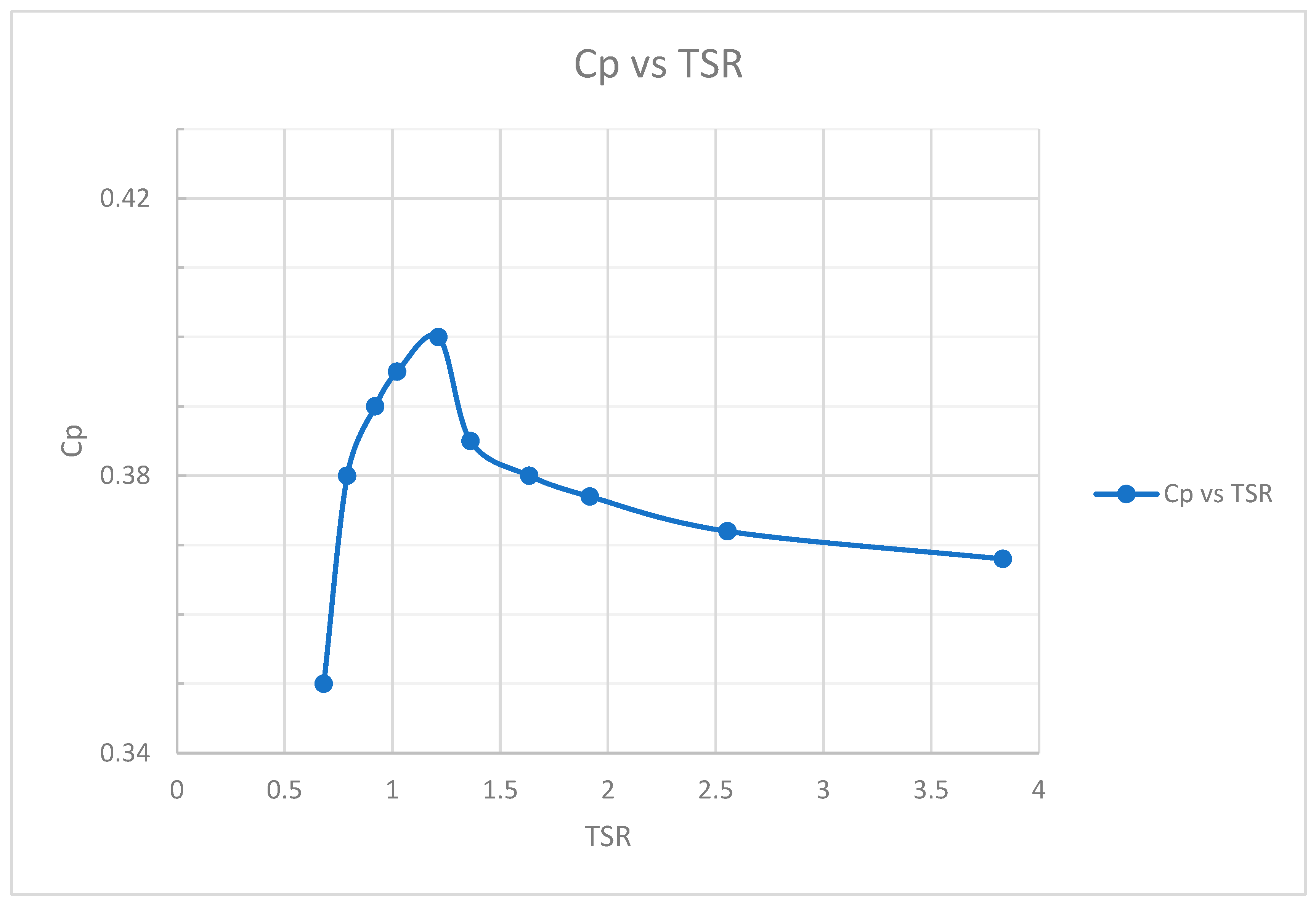
2.4. Performance Characteristics of Marine Turbines

Turbine performance is traditionally represented in terms of the tip-speed ratio (TSR), available power (Pavailabe), and power coefficient (Cp) according to Equations (4)–(6), respectively.
C P = P turbine   P available   = T ω 1 / 2 ρ AU 3
TSR = R ω U
P available   = 1 2 × ρ × A   ×   U 3
where U is the free stream speed (m/s), R is the radius of the turbine’s rotation (m), ω is the rotational speed of the turbine, Pturbine is the power generated by the turbine (W), ρ is the water density (kg/m3), and A is the turbine’s swept area (m2).

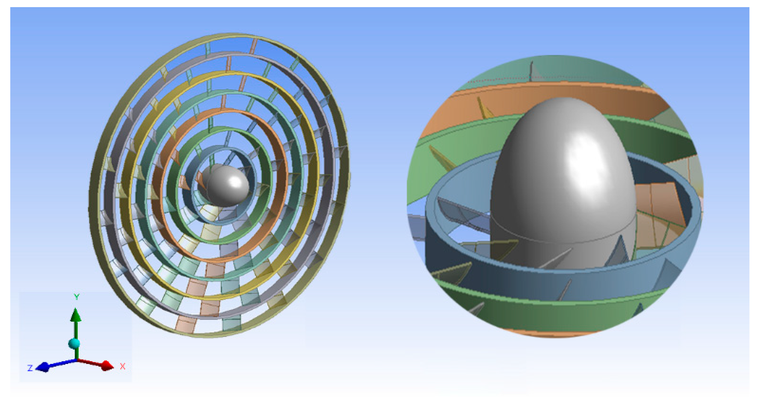
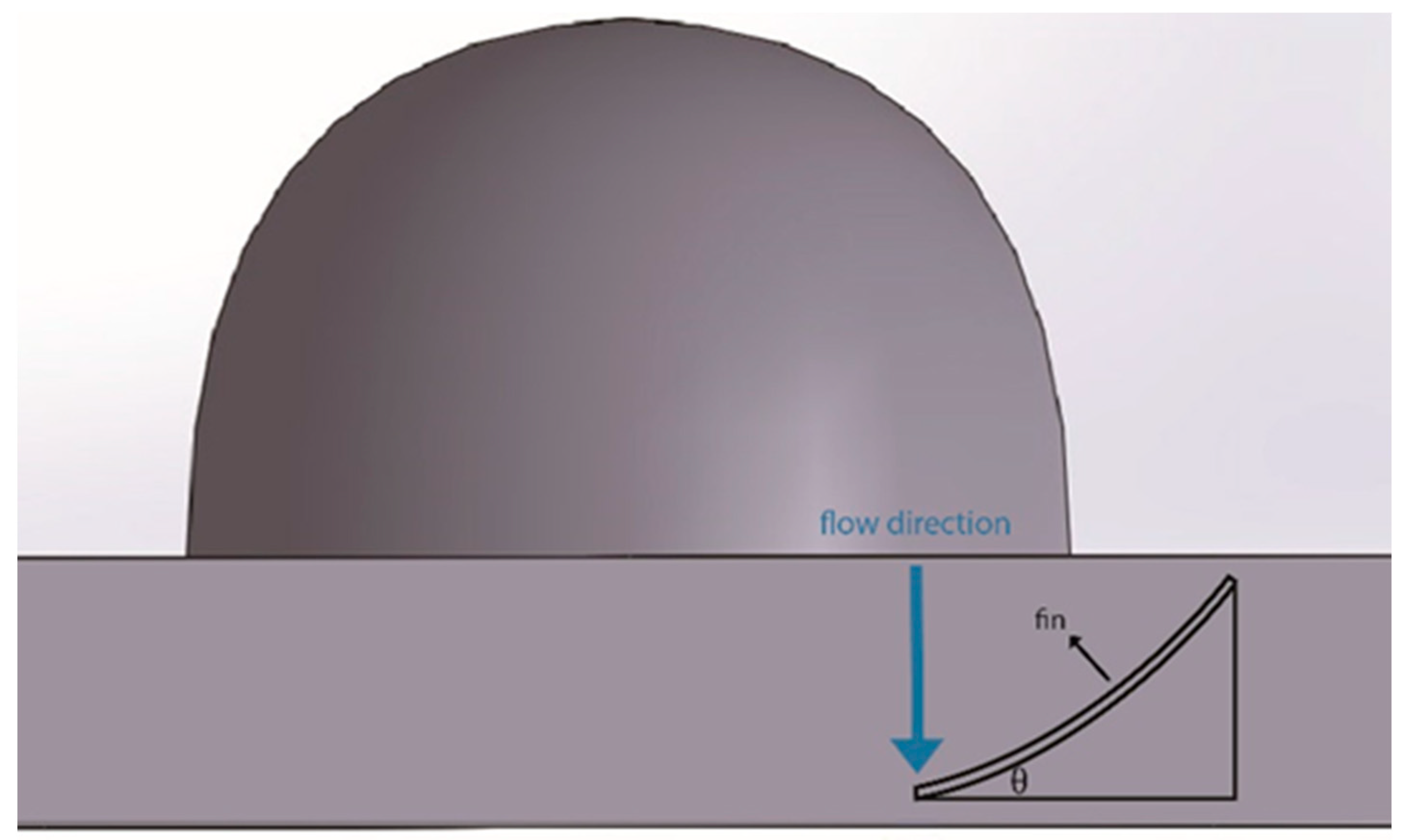
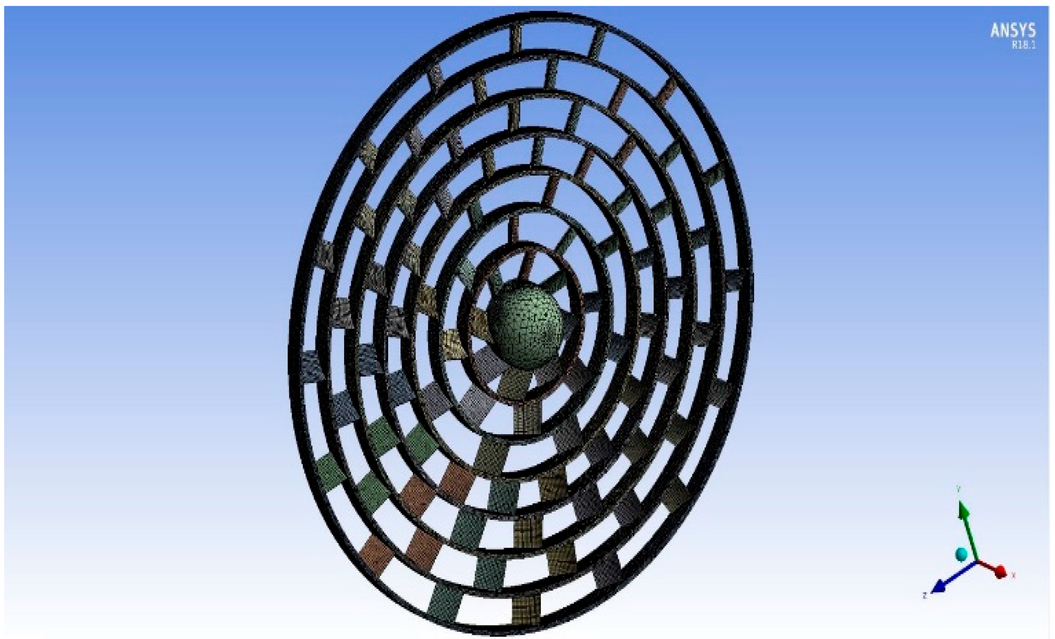
2.5. Fin-Ring Turbine 3D Model

The hydrodynamic performance of the fin-ring turbine [28] is numerically predicted by CFD simulations in this paper using ANSYS Fluent 18.1 software. In [36], the description of the benchmark design model geometry is presented and discussed. The benchmark design 3D model was created using the ANSYS Design modeler.
The fin-ring turbine 3D model has 7 rings with 88 fins and a solid center hub. The outside rings have 16 fins connecting the rings and, on the inside, it drops to 8 fins per ring. The fins are flat plates with a camber (l) and are oriented at a pitch angle (θ) to the direction of the flow. They act as hydrofoil sections that create drag and rotate the turbine to generate green electricity. The 3D turbine model’s isometric view and fins are shown in Figure 1 and Figure 2.
The fin pitch angle (θ) is defined as the angle between the fin and the virtual line perpendicular to the water current flow direction, as shown in Figure 2. The fins are distributed over 7 rings in a way that makes every fin in each ring situated in the middle radial space between two successive fins in the next ring. Due to the definition of the fin pitch angle (θ), the angle has a fixed value of 37.5° through all the rings [28,36].
The configuration of the design used in this work, including the dimensions of the turbine and fins, is summarized in Table 1.

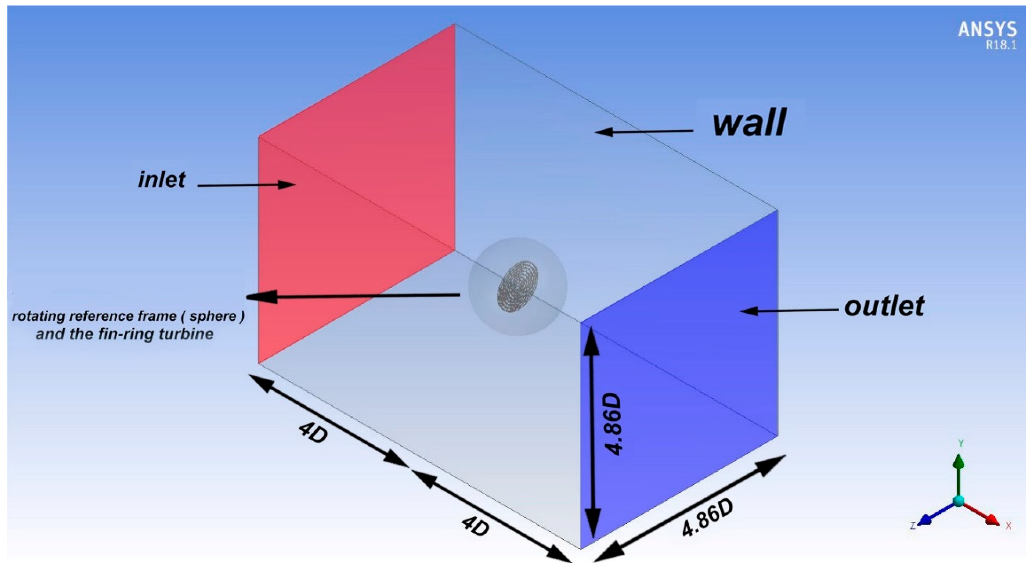
2.5.1. Computational Domain and Boundary Conditions
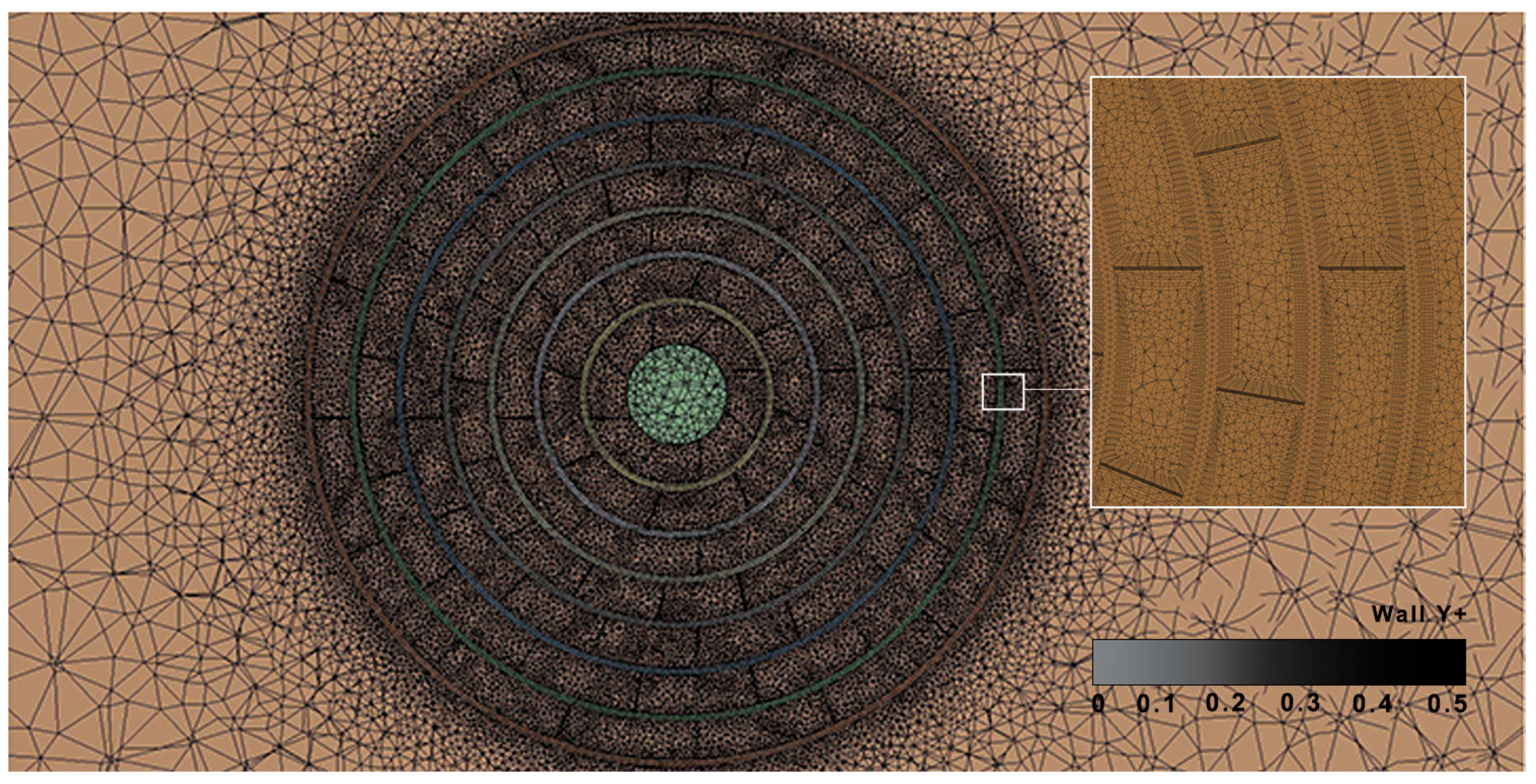
The rectangular computational domain is widely adopted when it comes to modeling open water flow and turbines. Thus, the computational domain is designed with a rectangular cross-section of 12 m × 12 m and a total length of L = 20 m. The fin-ring turbine was placed longitudinally at a distance of 4D from the inlet and the outlet of the domain where D is the diameter of the turbine, as shown in Figure 3.
For the flow field upstream of the turbine, no complex flow features are expected. However, the inlet section needs to be long enough for the flow to be fully developed before reaching the turbine. This requires extensive computational resources and comes with the price of increasing the computational time. The computational domain dimensions are considered within the recommended values provided by [34].
The computational domain is divided into two sections: the fixed domain and a rotating area bounded by the interface. A rotating frame of reference is selected to simulate the rotation of the turbine to save computational time. The rotating enclosure is chosen to be a sphere. This approach simulates the rotation of the turbine at different constant angular speeds without physically rotating the whole grid. This is achieved by applying the governing equations to the domain in a frame of reference that rotates with the turbine, while the outer domain remains referenced to a stationary coordinate system.
The slip boundary condition is used in the bottom, side, and top walls. The interface boundary condition is adopted between the chosen sphere and the fin-ring turbine. The inlet condition (red surface) is set with a uniform and steady current. The outlet (blue surface) is set with outlet pressure conditions, and the static gauge pressure is considered to be 101,300 Pa.
The solver settings and discretization method for the equations are shown in Table 2.
The maximum number of iterations for the convergence of governing equations is set to 1000, which is enough for all the governing equations being solved to reach convergence. The convergence relative percentage error (RPE) is set to the order of magnitude 1 × 10⁻², which is the default recommended by ANSYS Fluent 18.1. The RPE is the difference between the calculated value of a parameter and the guessed value of the same parameter at each iteration.

2.5.2. Mesh

The unstructured mesh created with ANSYS-CFX MESH is suitable for the type of problem under consideration while avoiding all complexities associated with other types of meshes. A grid sensitivity study was conducted to choose the optimal mesh, considering the best power coefficient (Cp) and fewest number of elements, as shown in Table 3.
After conducting the sensitivity study, the final mesh used in this work is of a fine, 3D tetrahedron element type, with 4,143,649 elements. There is no need to use the very fine mesh, since it uses tremendous computational power for an improvement in the Cp of only 1%. The body-sizing function was applied to the rectangular domain, limiting the maximum element size to 0.35 m, while the maximum element size was limited to 0.78 m for the turbine. To capture the exact flow behavior near the walls, the prism layer was used to resolve the boundary layer. In grid generation, the normal non-dimensional distance y+ of the first cell layer adjacent to the turbine wall was kept below 0.5 to resolve the near wall boundary layer, as shown in Figure 4. The reported quality of the mesh elements is the following: the average skewness is 0.22, maximum skewness is 0.82, average aspect ratio is 1.8, maximum aspect ratio is 11.2, average orthogonal quality is 0.86, and maximum orthogonal quality is 0.99. The mesh is shown in Figure 5.

3. Results and Discussion

In this section, the numerical results of the hydrodynamic performance of the fin-ring turbine used in this work are presented and discussed. The results include the turbine’s output power and power coefficient (Cp) generated for two different current speeds, plotted against a range of rpms. In addition, power test results for an installation of two identical prototypes of the fin-ring turbine are shown for validation, as obtained by [36]. The power output delivered by the two tested turbines is extracted from the power tests for validation. In addition, the turbulence model sensitivity study between the two turbulence models discussed previously in Section 2 is presented to choose the best turbulence model for the novel turbine’s design. The comparison is based on the performance curves of the two turbines. Moreover, the turbine’s Cp vs. tip-speed ratio (TSR) performance curve is constructed and presented to provide a complete overview of the turbine’s performance for a logical range of different marine current speeds. Finally, the potential for extracting hydrokinetic power using the turbine in three areas on the Spanish coast is explored and discussed.
Figure 6 shows the numerical results of the power generated by the fin-ring turbine design referred to in Table 2 vs. a range of rpms varying from 1 to 26 at current speeds of 6 ft/s (1.83 m/s) and 6.7 ft/s (2.04 m/s). The generated power increases with the rpm until it reaches a maximum, and then it inverses downwards. The results show a maximum power of 5.78 kW, obtained at an rpm of 15 for the lower current speed, and a maximum power of 7.96 kW, obtained at an rpm of 19 for the higher current speed. The working rotational speed corresponding to the maximum power changed by almost 27%, from 15 rpm to 19 rpm. This proves that the turbine is working in a low rpm range, which reduces the possibility of cavitation. These results are presented for the specific design configuration presented in Table 2. However, more designs can be generated to explore the influence of the turbine’s input design parameters: fin pitch angle (θ), camber (l), and ASR on the generated Cp.
The prototype of the turbine was tested in the Gulf of Mexico as a fully functional submerged generation support structure by pulling it with a boat to simulate various ocean stream velocities [28]. Figure 7 shows the power test results for the generated power delivered by two prototypes of the fin-ring turbine pulled for 2 h and at various forward speeds. From the power tests, the two turbines generated an average total power of 11.8 kW after considerable losses with 40 % efficiency at a current speed of 6 ft/s (1.83 m/s) and 16.4 kW with the same efficiency but at a speed of 6.7 ft/s (2.04 m/s).
The CFD results were validated with the field test results in terms of the turbine’s peak power coefficient Cp and output power Poutput. The relative percentage error (RPE) between the CFD and field test results can be calculated using Equation (7).
RPE   % =   CFD   results     Field .   results   Field .   results   × 100
The comparison reveals the accuracy of the results, since the error is 2% and 3%, respectively. The comparison is presented in Table 4.
This result particularly demonstrates the accuracy of the turbine’s CFD numerical model, which could encourage other researchers to replicate the design for subsequent analyses and future studies.
For all the previous simulation cases performed, the turbulence model used was the k-ε standard model. However, this model deals with turbulent flows only, which means the laminar and transition zone effect was not captured and included in the results. Thus, another suitable turbulence model must be used to capture and include the laminar and transition zone effect. The turbulence model most frequently used for such cases is the k-kl-ω. Figure 8 shows the comparison between the turbine’s generated Poutput using the k-ε model and the k-kl-ω for a current speed of 1.83 m/s. The comparison shows that the max Poutput of the turbine has increased by 1% to a value of 5.9 kW and the Cp to a value of 0.40. The sensitivity study highlights the advantage of using the k-kl-ω model over the k-ε model for the turbine presented in this work. Moreover, it proves that the dominant flow around the turbine is laminar, as the laminar/turbulent transition exerts considerable influence on the loss of flow’s kinetic energy, which affects the Cp of the turbine.
The main goal of this study is to explore the potential for hydrokinetic power on the Spanish coast using a suitable turbine that can operate efficiently at lower current speeds. Therefore, the values of the average current speed around the Iberian Peninsula, the Canary Islands, and the Balearic Islands in 2022 have been studied. Around the Iberian Peninsula and islands, the currents take different values. Three areas have been selected as representative of low, medium, and high values of current speed. The lowest values of current speed occur in areas like the Gulf of Cádiz, located in the eastern sector of the North Atlantic Ocean, to the southwest of the Iberian Peninsula. Medium values of current speed are in areas like Cape Palos near Cartagena, Spain. The highest current values can be found in areas like Cape Begur on the northern Mediterranean coast [29]. These values are shown in Table 5.
To this end, it is more practical to evaluate the hydrodynamic performance of the fin-ring turbine at any current speed based on the power coefficient (Cp) vs. the tip-speed ratio (TSR) curve. The curve defines the logical range of marine current speeds at which the fin-ring turbine will perform satisfactorily and efficiently. Based on the turbine’s performance curve, the potential for extracting hydrokinetic power in three regions on the Spanish coast is explored and discussed.
To construct the Cp vs. TSR performance curve, more current speeds must be established. Thus, more CFD simulations have been conducted for speed values ranging from 0.4 m/s to 3 m/s. For each current speed, the maximum Poutput is calculated from CFD simulations, and the corresponding rotational speed ω is noted. Then, the Pavailabe, Cp, and TSR are calculated using Equations (4)–(6), respectively. The Cp vs. TSR turbine performance curve is shown in Figure 9.
The performance curve shows that the fin-ring turbine’s Cp increases with higher TSRs until it reaches the peak value of 0.4 at a TSR of 1.213 with a current speed of 2 m/s. Then, it decreases by 5% to a value of 0.38 at TSR = 1.64 with current speed of 1.25 m/s, creating a narrow performance band shape for all the current speed values in between these values. After this, the Cp traces a linear downward movement with a low slope until it reaches a minimum value of 0.368, 8% lower than the peak value at a TSR of 3.83 with a current speed of 0.4 m/s.
This performance curve highlights the advantages of the unique design of the fin-ring turbine. Lowering the current speed from 2 m/s to 1.25 m/s, which is a 37.5% reduction in value, only decreased the Cp by 5%, while reducing the current speed by 80% to a value of 0.4 m/s reduced the peak value by 8%.
Based on this unique turbine’s performance, the potential for extracting hydrokinetic power in lower current areas is feasible. Using the turbine in three areas of the Spanish coast with different current values is investigated.
The three areas are considered in increasing order for their current values, starting from the lowest value of 0.45 m/s in Cádiz, the average value of 0.55 m/s in Cape Palos, and the maximum value of 0.81 m/s in Cape Begur [29]. Notably, the Cp of the turbine in these three places varies from 0.365 to 0.375, approximately 91.25% and 93.75%, respectively, of the peak Cp value of 0.4. This proves the adequate performance of the turbine in lower current values, hence the suitability of using it in lower current areas.

4. Conclusions

In this study, CFD simulations of the hydrodynamic performance of a fin-ring marine current turbine have been carried out and validated using test data available in the literature. A comparison of the results reveals the accuracy of the simulations, as discussed earlier.
Validated results are obtained for two different current speeds with a range of rpms. A maximum power coefficient (Cp) of nearly 40% is obtained at the two current speeds, which closely agrees with the maximum Cp obtained from the field power tests. The turbine generates power in a low rpm range, which eliminates the odds of cavitation.
The results of the mesh independency study revealed that the fine mesh provides a viable compromise between computational resources and accuracy. The optimal fine mesh generated a peak Cp of 0.392, which is only 1% lower than the peak Cp of the very fine mesh (0.401). Notably, the fine mesh required 15% fewer mesh elements to achieve these results, resulting in a significant reduction in computational resources without sacrificing much accuracy. Overall, these findings underscore the importance of carefully balancing mesh resolution and computational cost in numerical simulations, particularly in limited resource settings.
The fin-ring turbine operates mostly in a laminar regime flow. Thus, the turbine’s maximum Cp is increased by 1% when capturing the laminar/turbulent transition due to using the k-kl-ω model. This proves the suitability of this model for the existing turbine and other turbines that operate under the same conditions.
The Cp vs. TSR performance curve was constructed to evaluate the hydrodynamic performance of the fin-ring turbine on a range of current speeds. The turbine’s peak Cp value of 0.4 at a current speed of 2 m/s was reduced only by 8% to a value of 0.368 at the lowest current of 0.4 m/s. The narrow shape performance curve highlights the advantages of the fin-ring turbine’s unique design.
Based on this unique turbine’s performance curve, the potential for extracting hydrokinetic power in three areas on the Spanish coast has been explored. Cadiz, Cape Palos, and Cape Begur, with low, average, and high current values of 0.45 m/s, 0.55 m/s, and 0.81 m/s, respectively, serve the purpose of testing the turbine’s performance. The different CFD numerical results show that the turbine’s peak Cp slightly decreased by 8.75% and 6.25% from 0.4. This proves that the turbine’s performance is not highly sensitive to the lower variation of current speed, making it suitable for the lower current areas found in locations like the Spanish coast.
Our results are a preamble to an optimization study on the current design of the proposed fin-ring turbine. The study will cover varying relevant design parameters to improve the hydrodynamic efficiency of the turbine. These parameters will include the fin pitch angle, fin camber, fin aspect ratio, and number of rings.

Author Contributions

Conceptualization, M.I.I. and M.J.L.; methodology, M.I.I.; software, M.I.I.; validation, M.I.I.; formal analysis, M.I.I.; writing—original draft preparation, M.I.I. and M.J.L.; writing—review and editing, M.I.I. and M.J.L.; visualization, M.I.I. and M.J.L.; supervision. M.J.L.; All authors have read and agreed to the published version of the manuscript.

Funding

This research is funded by Project PID2019-108336GB-I00 financed by MCIN/AEI/10.13039/501100011033.

Institutional Review Board Statement

Not applicable.

Informed Consent Statement

Not applicable.

Data Availability Statement

Not applicable.

Conflicts of Interest

The authors declare no conflict of interest.

Appendix A

The k- ε model used in this work contains the following expressions:
The following (simplified) model equation for k is commonly used:
ρ k t +   div ρ k U = div μ t σ k grad k   + 2 μ t E i j · E i j ρ ε
The following (simplified) model equation for ε is commonly used:
ρ ε t +   div ρ ε U =   div μ t σ ε grad ε + C 1 ε ε k 2 μ t E i j · E i j C 2 ε ρ ε 2 k
where k is the turbulent kinetic energy per unit mass, ε is the dissipation rate of k , U is the mean velocity component at the x direction, μ t is the turbulent viscosity, E i j is the mean rate of deformation tensor, σ k and σ ε are the Prandtl numbers which connect the diffusivity of k and ε to the eddy viscosity, and C 1 ε and C 2 ε are the model constants with values of 1.44 and 1.92, respectively.
Also,
μ t = C μ k 2 ε , C μ = 0.09 , E i j = 1 2 U i x j + U j x i , σ k = 1 ,   and   σ ε = 1.3
The k-kl-ω transition model used in this work contains the following expressions:
The following three equations are commonly used:
  • Transport equation for turbulent kinetic energy, kt
    D k t D t = P k T + R B P + R N A T ω k t D t + x j ν + α T σ k k t x j
  • Transport equation for laminar kinetic energy, k L
    D k L D t = P k L R B P R N A T D L + x j ν k L x j
  • Transport equation for inverse turbulent time turbulent scalar diffusivity, f W is the inviscid near-wall scale, ω , defined as ω = ε / k t
    D ω D t = C ω 1 ω k t P k T + C ω R f W 1 ω k t R B P + R N A T C ω 2 ω 2 + C ω 3 f ω α T f W 2 k t d 3 + x j ν + α T σ ω ω x j
The near-wall dissipation is given by
D t = 2 v k t x j k t x j D L = 2 v k L x j k L x j
The damping function f W is defined as
f W = λ e f f λ T
where D t and D L are the near-wall dissipation terms for k t and k L , respectively. P K L is the production of laminar kinetic energy from large-scale turbulent fluctuations; P K t is the production of turbulent kinetic energy from large-scale turbulent fluctuations; R B P represents the averaged effect of the breakdown of streamwise fluctuations into turbulence during bypass transition; R N A T is the natural transition production term indicating the breakdown to turbulence due to instabilities; α T is the turbulent scalar diffusivity; f W is the inviscid near-wall scale, ω , defined as ω = ε / k t damping function; f ω is the boundary layer wake term damping function; λ T is the turbulent length scale; and λ e f f is the effective length.
The values of the model constants are: C ω 1 = 0.44 , C ω 2 = 0.92 , C ω 3 = 0.3 , C ω R = 1.5 , σ k = 1 , and σ ω = 1.17 .

References

  1. Gordon, M.; Weber, M. Global Energy Demand to Grow 47% by 2050, with Oil Still Top Source: US EIA. 2021. Available online: https://www.spglobal.com/commodityinsights/en/market-insights/latest-news/oil/100621-global-energy-demand-to-grow-47-by-2050-with-oil-still-top-source-us-eia (accessed on 1 January 2023).
  2. Bentley, R.W. Global Oil & Gas Depletion: An Overview. Energy Policy 2002, 30, 189–205. [Google Scholar] [CrossRef]
  3. Konrad, K. An Unexpected Future for Oil and Gas. Max Planck Research Magazine. 2022. Available online: https://www.mpg.de/19037054/an-unexpected-future-for-oil-and-gas (accessed on 1 January 2023).
  4. Esteban, M.D.; Espada, J.M.; Ortega, J.M.; López-Gutiérrez, J.-S.; Negro, V. What about Marine Renewable Energies in Spain? J. Mar. Sci. Eng. 2019, 7, 249. [Google Scholar] [CrossRef]
  5. Haas, K. Assessment of Energy Production Potential from Ocean Currents along the United States Coastline; Georgia Institute of Technology: Atlanta, GA, USA, 2013. [Google Scholar]
  6. Duerr, A.E.S.; Dhanak, M.R. Hydrokinetic Power Resource Assessment of the Florida Current. In Proceedings of the OCEANS 2010 MTS/IEEE SEATTLE, Seattle, WA, USA, 20–23 September 2010. [Google Scholar] [CrossRef]
  7. Chen, F. Kuroshio Power Plant Development Plan. Renew. Sustain. Energy Rev. 2010, 14, 2655–2668. [Google Scholar] [CrossRef]
  8. Brooks, D.A. The Hydrokinetic Power Resource in a Tidal Estuary: The Kennebec River of the Central Maine Coast. Renew. Energy 2011, 36, 1492–1501. [Google Scholar] [CrossRef]
  9. Xia, J.; Falconer, R.A.; Lin, B. Numerical Model Assessment of Tidal Stream Energy Resources in the Severn Estuary, UK. Proc. Inst. Mech. Eng. Part A J. Power Energy 2010, 224, 969–983. [Google Scholar] [CrossRef]
  10. Draper, S.; Adcock, T.A.A.; Borthwick, A.G.L.; Houlsby, G.T. Estimate of the Tidal Stream Power Resource of the Pentland Firth. Renew. Energy 2014, 63, 650–657. [Google Scholar] [CrossRef]
  11. Rashid, A. Status and Potentials of Tidal In-Stream Energy Resources in the Southern Coasts of Iran: A Case Study. Renew. Sustain. Energy Rev. 2012, 16, 6668–6677. [Google Scholar] [CrossRef]
  12. Byun, D.-S.; Hart, D.; Jeong, W.-J. Tidal Current Energy Resources off the South and West Coasts of Korea: Preliminary Observation-Derived Estimates. Energies 2013, 6, 566–578. [Google Scholar] [CrossRef]
  13. Calero Quesada, M.C.; García Lafuente, J.; Sánchez Garrido, J.C.; Sammartino, S.; Delgado, J. Energy of Marine Currents in the Strait of Gibraltar and Its Potential as a Renewable Energy Resource. Renew. Sustain. Energy Rev. 2014, 34, 98–109. [Google Scholar] [CrossRef]
  14. Mestres, M.; Cerralbo, P.; Grifoll, M.; Sierra, J.P.; Espino, M. Modelling Assessment of the Tidal Stream Resource in the Ria of Ferrol (NW Spain) Using a Year-Long Simulation. Renew. Energy 2019, 131, 811–817. [Google Scholar] [CrossRef]
  15. Carballo, R.; Iglesias, G.; Castro, A. Numerical Model Evaluation of Tidal Stream Energy Resources in the Ría de Muros (NW Spain). Renew. Energy 2009, 34, 1517–1524. [Google Scholar] [CrossRef]
  16. Mestres, M.; Griñó, M.; Sierra, J.P.; Mösso, C. Analysis of the Optimal Deployment Location for Tidal Energy Converters in the Mesotidal Ria de Vigo (NW Spain). Energy 2016, 115, 1179–1187. [Google Scholar] [CrossRef]
  17. Ramos, V.; Carballo, R.; Álvarez, M.; Sánchez, M.; Iglesias, G. A Port towards Energy Self-Sufficiency Using Tidal Stream Power. Energy 2014, 71, 432–444. [Google Scholar] [CrossRef]
  18. Ramos, V.; Iglesias, G. Performance Assessment of Tidal Stream Turbines: A Parametric Approach. Energy Convers. Manag. 2013, 69, 49–57. [Google Scholar] [CrossRef]
  19. Legaz, M.J.; Soares, C.G. Evaluation of various wave energy converters in the bay of Cádiz. Brodogr. Teor. I Praksa Brodogr. I Pomor. Teh. 2022, 73, 57–88. [Google Scholar] [CrossRef]
  20. Behrouzi, F.; Maimun, A.; Nakisa, M. Review of Various Designs and Development in Hydropower Turbines. Int. J. Mech. Aerosp. Ind. Mechatron. Manuf. Eng. 2014, 8, 293–297. [Google Scholar]
  21. Kusakana, K.; Vermaak, H.J. Hydrokinetic Power Generation for Rural Electricity Supply: Case of South Africa. Renew. Energy 2013, 55, 467–473. [Google Scholar] [CrossRef]
  22. Tian, W.; Song, B.; VanZwieten, J.H.; Pyakurel, P.; Li, Y. Numerical Simulations of a Horizontal Axis Water Turbine Designed for Underwater Mooring Platforms. Int. J. Nav. Archit. Ocean. Eng. 2016, 8, 73–82. [Google Scholar] [CrossRef]
  23. Elghali, S.E.B.; Benbouzid, M.E.H.; Charpentier, J.F.; Ahmed-Ali, T.; Munteanu, I. High-Order Sliding Mode Control of a Marine Current Turbine Driven Permanent Magnet Synchronous Generator. In Proceedings of the 2009 IEEE International Electric Machines and Drives Conference, Miami, FL, USA, 3–6 May 2009. [Google Scholar] [CrossRef]
  24. Hammerfest, A.H. Renewable Energy from Tidal Currents; Andritz Hydro: Charlotte, NC, USA, 2009. [Google Scholar]
  25. Thake, J. Development, Installation and Testing of a Large Scale Tidal Current Turbine. I T Power. 2005. Available online: https://www.osti.gov/etdeweb/biblio/20714897 (accessed on 1 January 2023).
  26. Gaden, D.L.F.; Bibeau, E.L. A Numerical Investigation into the Effect of Diffusers on the Performance of Hydro Kinetic Turbines Using a Validated Momentum Source Turbine Model. Renew. Energy 2010, 35, 1152–1158. [Google Scholar] [CrossRef]
  27. Kramm, G.; Sellhorst, G.; Ross, H.K.; Cooney, J.; Dlugi, R.; Mölders, N. On the Maximum of Wind Power Efficiency. J. Power Energy Eng. 2016, 4, 41001. [Google Scholar] [CrossRef]
  28. Bolin, W. Ocean Stream Power Generation: Unlocking a Source of Vast, Continuous, Renewable Energy. In Proceedings of the 2nd Marine Energy Technology Symposium, Seattle, WA, USA, 15–18 April 2014. [Google Scholar]
  29. Puertos del Estado. Predicción de Oleaje, Nivel del Mar; Boyas y Mareógrafos. Available online: https://www.puertos.es/en-us/oceanografia/Pages/portus.aspx (accessed on 1 January 2023).
  30. Batten, W.M.J.; Bahaj, A.S.; Molland, A.F.; Chaplin, J.R. Experimentally Validated Numerical Method for the Hydrodynamic Design of Horizontal Axis Tidal Turbines. Ocean. Eng. 2007, 34, 1013–1020. [Google Scholar] [CrossRef]
  31. Myers, L.; Bahaj, A.S. Power output performance characteristics of a horizontal axis marine current turbine. Renew. Energy 2006, 31, 211–222. [Google Scholar] [CrossRef]
  32. Lawson, M.J.; Li, Y.; Sale, D.C. Development and Verification of a Computational Fluid Dynamics Model of a Horizontal-Axis Tidal Current Turbine. In Proceedings of the International Conference on Ocean, Offshore and Arctic Engineering (ASME 2011), Rotterdam, The Netherlands, 19–24 June 2011. [Google Scholar] [CrossRef]
  33. Pape, A.L.; Lecanu, J. 3D Navier-Stokes Computations of a Stall-Regulated Wind Turbine. Wind Energy 2004, 7, 309–324. [Google Scholar] [CrossRef]
  34. Helal, M.M.; Ahmed, T.M.; Banawan, A.A.; Kotb, M.A. Numerical Prediction of the Performance of Marine Propellers Using Computational Fluid Dynamics Simulation with Transition-Sensitive Turbulence Model. Proc. Inst. Mech. Eng. Part M J. Eng. Marit. Environ. 2018, 233, 515–527. [Google Scholar] [CrossRef]
  35. Launder, B.E.; Spalding, D.B. The Numerical Computation of Turbulent Flows. Comput. Methods Appl. Mech. Eng. 1974, 3, 269–289. [Google Scholar] [CrossRef]
  36. Ibrahim, M.I.; Hamed, T.M.; Banawan, A.A. CFD Simulation of the Hydrodynamic Performance of a Fin-Ring Marine Current Turbine. In Sustainable Development and Innovations in Marine Technologies, Proceedings of the 18th International Congress of the Maritime Association of the Mediterranean (IMAM 2019), Varna, Bulgaria, 9–11 September 2019; CRC Press: Boca Raton, FL, USA; pp. 545–551. [CrossRef]
Figure 1. Design and geometry of the fin-ring turbine.
Jmse 11 00942 g001
Figure 2. Fin pitch angle θ and camber [36].
Jmse 11 00942 g002
Figure 3. Computational domain and boundaries [36].
Jmse 11 00942 g003
Figure 4. Turbine wall y+ values.
Jmse 11 00942 g004
Figure 5. Fin-ring turbine unstructured mesh.
Jmse 11 00942 g005
Figure 6. Turbine output power vs. rpm at two different current speeds.
Jmse 11 00942 g006
Figure 7. Power test results for two prototype turbines [28].
Jmse 11 00942 g007
Figure 8. Poutput at current speed of 1.83 m/s using k-ε and k-kl-ω.
Jmse 11 00942 g008
Figure 9. Cp vs. TSR performance curve.
Jmse 11 00942 g009
Table 1. Characteristics of the fin-ring turbine reference design.
Characteristic of Fin-Ring Turbine
Number of ringsNrings7
Turbine diameter (outmost diameter)D2.44 m
Spacing between rings (fin height)S0.13 m
No. of finsNfins88
Fin pitch angleθ37.5°
Fin camber lengthl0.01 m
Fin aspect ratioASR0.82
Table 2. Solver settings and discretization method.
Solver Settings and Discretization Method
Solver typePressure-based (coupled)
Analysis typeSteady-state (totating frame of reference)
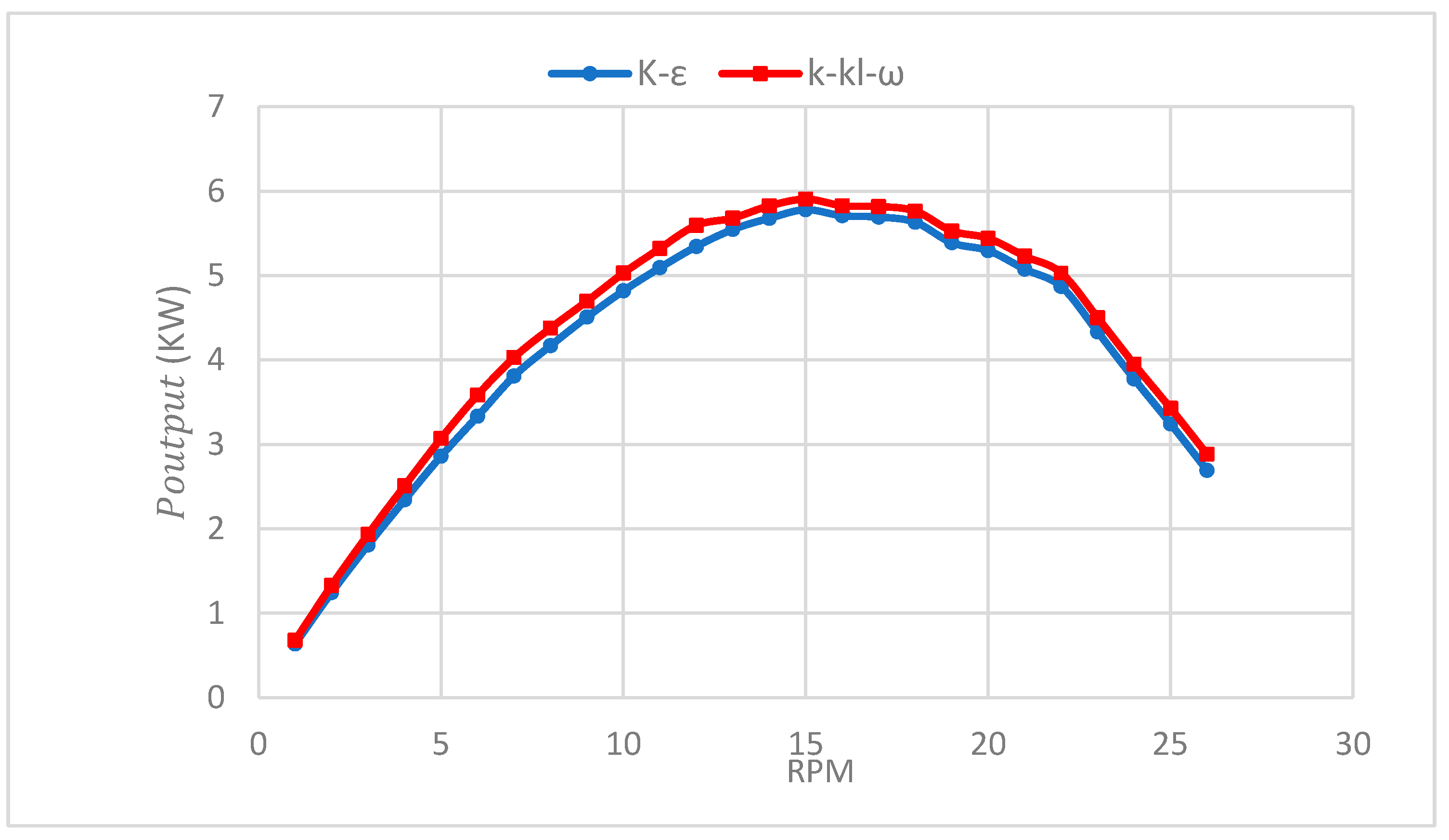
Turbulence modelStandard k-ε & K-kl-ω
Spatial discretization2nd order upwind for all the equations
Table 3. Mesh sensitivity study.
Mesh TypeCoarseFineVery Fine
No of elements1,093,2214,143,6496,153,212
Cp0.3500.3920.401
Table 4. CFD and power test results validation.
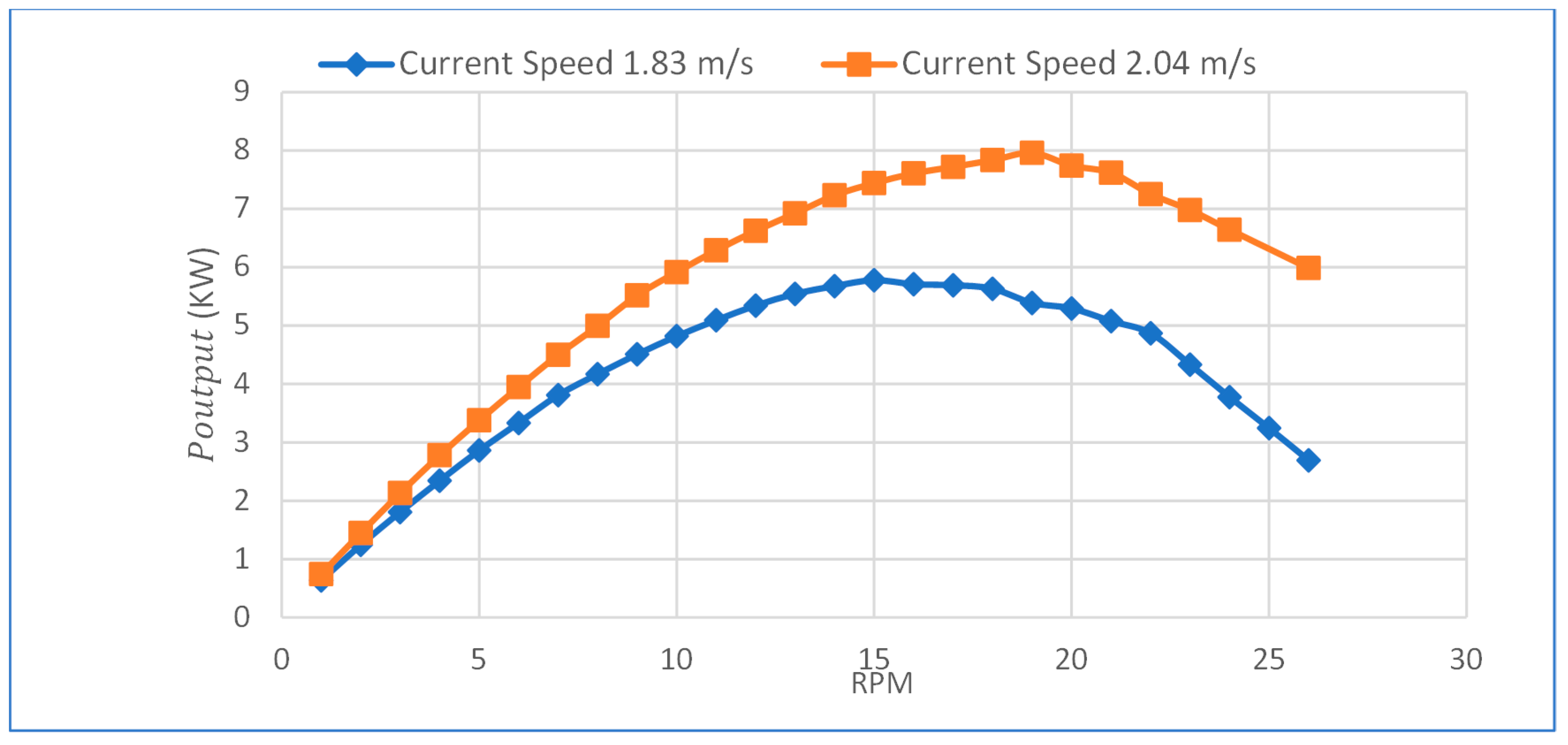
CFD and Power Test Results Validation
Current speed (m/s)1.832.04
Type of resultCFDFieldCFDField
Poutput (kW)5.785.97.968.2
Cp0.3920.400.3880.4
RPE (%)23
Table 5. Values of current speed on the Spanish coast [29].
Average Current Speed in m/s. Year 2022
Gulf of Cádiz buoyCape Palos buoyCape Begur buoy
0.450.550.88
Disclaimer/Publisher’s Note: The statements, opinions and data contained in all publications are solely those of the individual author(s) and contributor(s) and not of MDPI and/or the editor(s). MDPI and/or the editor(s) disclaim responsibility for any injury to people or property resulting from any ideas, methods, instructions or products referred to in the content.

