Numerical Analysis of Local Scour of the Offshore Wind Turbines in Taiwan

Abstract

Rapid expansions of the offshore wind industry have stimulated a renewed interest in the behavior of offshore wind turbines. Monopile, tripod, and jack-up wind turbines support most offshore wind turbines. These foundations are sensitive to scour, reducing their ultimate capacity and altering their dynamic response. However, the existing approaches ignore the seabed’s rheological properties in the scour process. This study focuses on the scour development around the wind turbine foundation in the Changhua wind farm in Taiwan. The simulation results explain the influence of different hydrodynamic mechanisms on the local scours in a cohesive fluid, such as regular waves, random waves, and constant currents. A newly non-Newtonian fluid model, the Discontinuous Bi-viscous Model (DBM), reproduces closet mud material nature without many empirical coefficients and an empirical formula. This new rheology model is integrated and coupled into the Splash3D model, which resolves the Navier–Stokes equations with a PLIC-VOF surface-tracking algorithm. The deformation of the scour hole, the backfilling, and the maximum scour depth are exhibited around the wind turbines. Waves, including regular and irregular waves, do not increase the scour depth compared with currents only. In the case of random wave–current coupling, the results present a signal of scour evolution. However, the scour depth is shallow at $0.033\le S/D\le 0.046$.

1. Introduction

Taiwan’s government actively promotes the utilization of renewable energy, aiming at strengthening energy autonomy and responding to climate change. The government aims for renewable energy to represent 20% of total power generation by 2025 and has set a target of 5.5 GW for offshore wind capacity. Offshore power generation has great potential for Taiwan [1]. The coastal areas of west Taiwan are rich in wind energy resources [2]. In addition, the Changhua area has the best wind energy potential on Taiwan’s west coast [3]. Currently, offshore wind turbines in Taiwan are installed underwater at 10 to 50 m.

Taiwan is in the Pacific Rim seismic zone. The Changhua offshore wind farm is located in western Taiwan. The seabed sediments are mostly sand and clay, which are relatively soft. Earthquakes occasionally take place, threatening the stability of offshore wind turbine foundations. Because of these special situations in Taiwan, offshore wind turbines not only sustain the impact of ocean currents and typhoon waves but also suffer the threats caused by the local scour of the seabed around the foundation piles.

In the Taiwan Strait, the waves are combined with currents and waves caused by typhoons. As for the wave field, this study provides a random wave field under the analysis of the JONSWAP spectrum in the Changhua Offshore wind farm. This wave field is the main input hydrodynamic condition when studying the local scour around the wind turbine systems.

Some offshore wind turbine foundations such as monopile, tripod, jacket, gravity base, and floating are popular worldwide. The adopted foundation solution depends on local seabed conditions, water depth, and financial constraints [4]. Monopiles are the most widely adopted substructure–foundation system for modern offshore wind farms located in shallow water depths (≤~40 m). Braced support structures (i.e., tripod and jacket) are more suitable for deeper water and heavier turbines [5,6]. For water depths greater than 50 m, floating platforms for wind turbines will impose many new design challenges [5,6].

In 2019, Chen studied the influence of ocean currents on the monopile and jacket foundations of offshore wind turbines in Taiwan [1]. Hydraulic model experiments were conducted to investigate the maximum scour depth and range around pillars in these foundations [1].

Many wind farms were built in environments characterized by the strong influence of tides, wind-induced currents, and waves. A scour hole will be developed if the wind turbines are placed without protection on an erodible seabed [7]. A real-time scour monitoring system can improve the safety of structures and afford cost-effective operations by preventing premature or unnecessary maintenance [8]. Scour in uniform sandy soils has been studied for decades. The role of waves on sand cannot be ignored [9]. Whitehouse monitored the scour development due to waves and currents around the installed foundations [10]. Offshore wind turbines founded on loose sands suffer significant stiffness reductions [11].

However, marine sediments of silty sand or sandy clay do not respond in the same way as sand. Marine sediment erosion is still uncertain and requires further investigation [12]. Scour prediction in cohesive or multi-modal soils (i.e., clay, silt, sand, gravel mixtures) is more complex. Typically, the scour process is much slower. The effect of scour depends on the time the structure will remain at the site [12]. Compared to mobile sand beds, mixtures of sand, silt, clay, and layered sediments should limit the extent of scour in complex soils. Further, clay soils can maintain steeper side slopes, affecting scour hole development [12].

The wind turbine foundations are sensitive to scour. Nonetheless, the present approaches ignore the seabed’s rheological properties in the scour process. This study focuses on scouring under the consideration of the rheology of the seabed sediment. In this study, a newly non-Newtonian fluid model, the Discontinuous Bi-viscous Model (DBM), reproduces closet mud material nature without many empirical coefficients and the empirical formula. This new rheology model is integrated and coupled into the Splash3D model, which resolves the Navier–Stokes equations with a PLIC-VOF surface-tracking algorithm.

The mathematical equations of Splash3D and rheological models are presented in Section 2. The model validations are shown in Section 3, including regular and random waves. Section 4 and Section 5 give the models’ applications. Section 4 contains four cases of local scour around a monopile wind turbine. Section 5 holds 4 cases of scouring process nearby a tripod and jack-up (4-leg) wind turbine. Section 6 and Section 7 give some discussions and conclusions from the study.

2. Numerical Model

2.1. Fluid Solver

This study adopted the Splash3D numerical model to solve breaking wave problems [13,14]. The model solves three-dimensional incompressible flow with Navier–Stokes equations. The free surface is tracked by the Volume-of-Fluid (VOF) method [15]. The domain is discretized by the Finite Volume Method (FVM) [16]. The turbulent effect is close to the Large Eddy Simulation (LES) model [17]. Detail description is presented in [18,19]. The mass conservation equation, the momentum conservation equation, and the VOF equation for the transport of the volume fraction α are defined as:

$$\frac{\partial \rho }{\partial t}+\nabla ·\left(\rho \mathit{u}\right)=0$$

(1)

$$\frac{\partial \rho \mathit{u}}{\partial t}+\nabla ·\left(\rho \mathit{u}\mathit{u}\right)=-\nabla P+\nabla ·{\mu }_e\left(\nabla \mathit{u}+{\left(\nabla \mathit{u}\right)}^T\right)+f_B$$

(2)

where the velocity vector is $\mathit{u}$, the pressure is $P$, the body force is $f_B$ (gravity force is an example), and the density is $\rho$. Equation (1) describes the transport of density, or more simply, the transport of different fluids within the domain. Equation (2) is a Eulerian expression of the conservation of fluid momentum. The effective viscosity ${\mu }_e$ is defined as:

$${\mu }_e=\mu \left(\dot{\gamma }\right)+{\mu }_t+{\mu }_m$$

(3)

where $\mu \left(\dot{\gamma }\right)$ is the rheology viscosity of the cohesive material calculated by the rheological model. ${\mu }_t$ is the viscosity of the sub-grid scale turbulence, of which a detailed calculation is presented in [18]. ${\mu }_m$ is the molecular viscosity.

Individual fluids are incompressible. The model considers multiple immiscible fluids (of different densities) within a domain and retains $\rho$ within the bracketed terms on the left-hand side of Equation (2). However, as the density of any fluid particle remains constant,

$$\frac{D\rho }{Dt}=0$$

(4)

and so:

$$\nabla ·\mathit{u}=0$$

(5)

2.2. Rheological Model

The Bingham model [20] is the simplest and the favorite mode to describe the rheological properties of the cohesive material. In addition, there are some other rheology models, namely, the modified Bingham model [21], the Bi-viscosity (or Bilinear) model [22], the Power law model [23], and the Herschel–Bulkley model [24].

A ball-measuring system measures the rheological characteristics of waste rock materials and mine tailings materials [25,26]. Both experiment data serials show that the shear stress of debris flow or mud flow materials can be divided into two regimes based on a yield shear rate, which defines the materials’ slip surface (yield surface). There is a distinct peak value of shear stress in a relatively low shear rate regime. After the peak value, an abrupt decrease in shear stress is observed [26]. This flow curve is also typically used in soil rheology [25]. This evidence about the distinct peak value and the abrupt decrease in shear stress promoted the development of the Discontinuous Bi-viscosity Model (DBM), which is indicated in detail in [19]. The DBM successfully predicted the mud flow and landslide tsunami in [18,19]. The DBM is written as:

$$\mu \left(\dot{\gamma }\right)=\left\{\begin{array}{c}{\mu }_A\gg \frac{{\tau }_y}{{\dot{\gamma }}_y} if \gamma <{\gamma }_y \\ {\mu }_B+\frac{{\tau }_y}{\dot{\gamma }} if \gamma \ge {\gamma }_y\end{array}\right.$$

(6)

where ${\mu }_A$ is the viscosity of the un-yield region, ${\mu }_B$ is the viscosity of the yield zone, ${\tau }_y$ is the yield stress, and ${\gamma }_y$ is the yield strain rate. The symbol $\gamma$ is the second invariant of the ${\gamma }_{ij}$, which is defined as $\gamma =\sqrt{\frac{1}{2}{\gamma }_{ij}{\gamma }_{ij}}$, where ${\gamma }_{ij}=\frac{\partial u_i}{\partial x_j}+\frac{\partial u_j}{\partial x_i}$. When the shear stress at the riverbed is lower than the yield stress, the cohesion of the bed material becomes important, and the riverbed behaves like a rigid boundary. Above the yield stress, the bed material acts like a Newtonian fluid. The boundary viscosity ${\mu }_A$ represents the viscosity of immobile bed material. When the boundary viscosity ${\mu }_A$ was set as ${10}^{10} \mathrm{Pa}·\mathrm{s},$ which is much larger than the dynamic viscosity of the water (${\mu }_m={10}^{-3} \mathrm{Pa}·\mathrm{s}$), the bed material was frozen like a rigid material. Four parameters (${\mu }_A$, ${\mu }_B$, ${\tau }_y$, and ${\gamma }_y$) are needed to define the properties of the bed material.

3. Model Validation

A train of regular and random waves is sent into the domains to prove the effectiveness of the internal source wavemaker model. The numerical waves are validated with the theoretical solutions at two wave gauges.

The predicted regular waves are compared with the theoretical solution of the second-order Stokes wave [27]:

$$\eta =\frac{H}{2}\cos \left(kx-\omega t\right)+\frac{H^{2}k}{16}\frac{\cosh kh}{{\sinh }^{3}kh}\left(2+\cosh 2kh\right)\cos 2\left(kx-\omega t\right)$$

(7)

The input parameters are wave height $H=6 \mathrm{m}$, wave period $T=8 \mathrm{s}$, and water depth $h=30 m$. According to the transitional water waves theory, the wave parameters are calculated as wavelength $L=96.054 \mathrm{m}$, wave number $k=0.065 {\mathrm{m}}^{-1}$, angular frequency $\omega =0.785{ \mathrm{s}}^{-1}$, and wave celerity $C=12.007 \mathrm{m}/\mathrm{s}$. The wave profile at two wave gauges is validated with Equation (7), shown in Figure 1. At x = 25 m (near the wave maker), the model wave height is 3.47% higher than the theoretical solution from Equation (7). However, the wave energy reduces when it propagates. The predicted wave height at x = 105 m is 8.3% smaller than the analytical solution. That means the wave height decreases by 14.13% per wavelength.

The random wave is simulated based on the averaged JONSWAP spectral, which was statistically analyzed from buoy data in the Taichung Sea, with the significant wave height $H_s=6 \mathrm{m}$, peak wave period $T_p=8 \mathrm{s}$, and water depth $h=30 \mathrm{m}$. Figure 2a compares the theoretical and the predicted JONSWAP spectrum at two wave gauges (x = 25 m and x = 105 m). The peak angular frequency is ${\omega }_p=\frac{2\pi }{T_p}=0.785 \left(\mathrm{rad}/\mathrm{s}\right)$. The simulated waves at Gauge 1 have identical peak angular frequency and frequency distribution; however, the spectrum reduces. This may be because the wave height decreases. At Gauge 2, the peak angular frequency shifts to 0.8 rad/s, and the spectrum decreases remarkably.

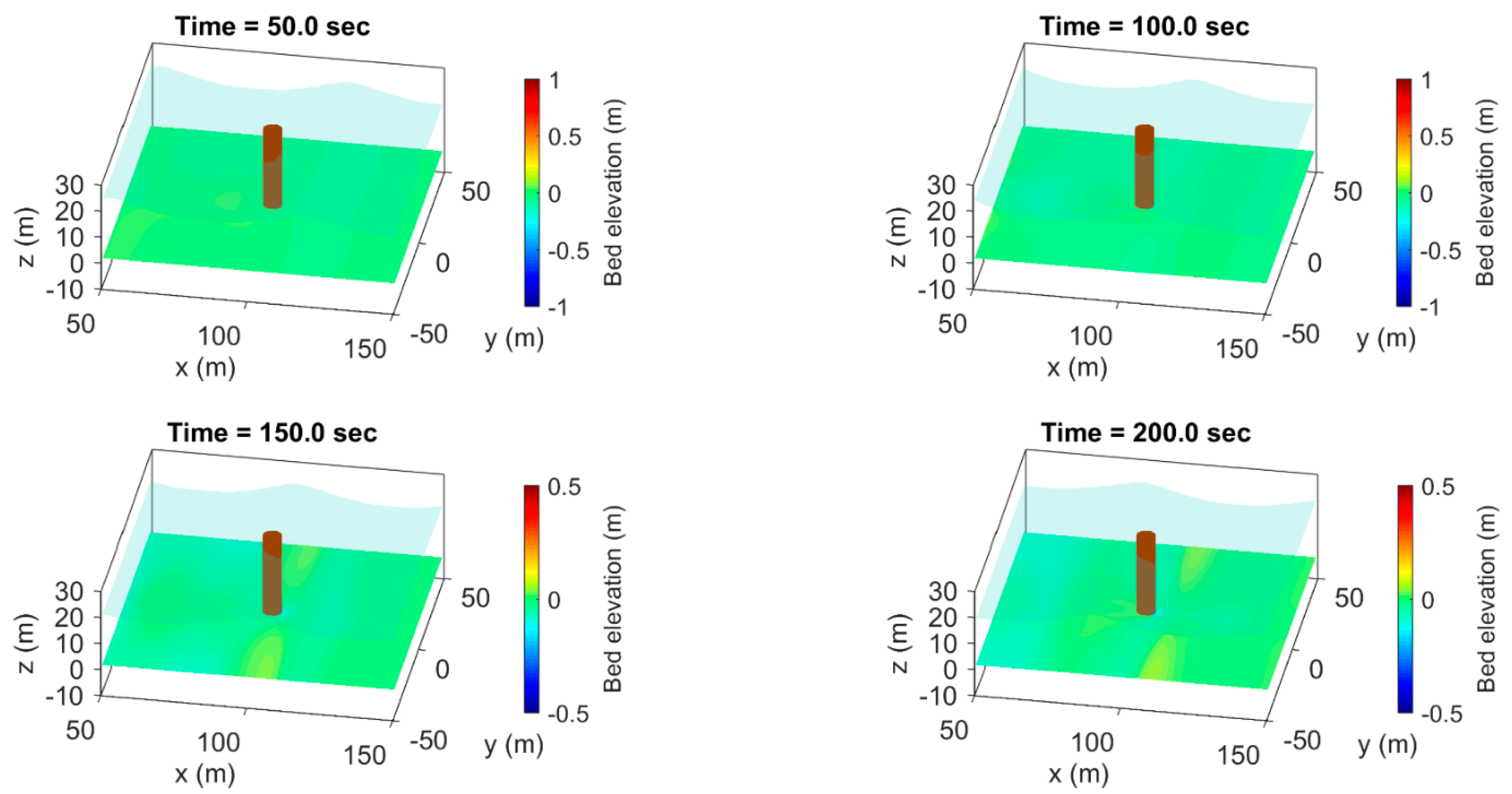
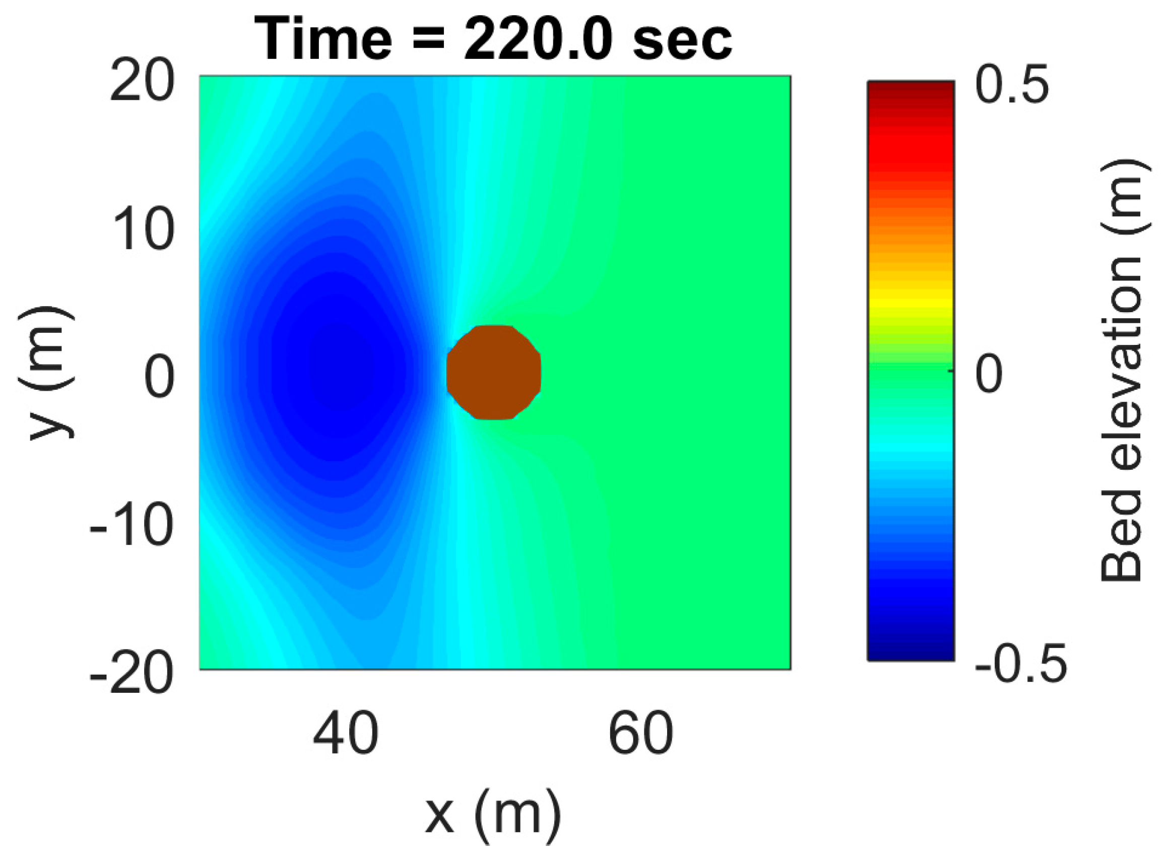
4. Monopile Wind Turbine

This study discusses the changes in the bottom bed and the development of local scour around a vertical pile under the effect of constant current, wave, and wave–current coupling. Four cases are conducted, with a normal and storm wave conditions numerical set-up in

Table 1. Four cases of monopile hydrodynamics.

Condition No.	Wave Type	Hydrodynamic Conditions
1	Constant ocean current	U = 1.0 m/s
2	Regular wave (100-year return period storm wave conditions)	Wave height H = 3.0 m Wave period T = 5.0 s
3	Regular wave—current (100-year return period storm wave conditions)	Wave height H = 3.0 m Wave period T = 5.0 s Current velocity U = 1.0 m/s
4	Irregular wave (100-year return period storm wave conditions)	Significant wave height Hs = 3.0 m Peak period Tp = 5.0 s

. These scenarios are run under storm conditions: the wave height is 4.0 m, and the wave period is 5.0 s. A wind turbine’s outer diameter is 6.0 m, and under 20.0 m water depth is presented.

For waves on ocean currents, the current is uniform over depth and horizontal distance and flows in the same direction as the waves. The angular frequency includes two terms [27]: $\omega =U_{0}k+\sqrt{gk\tanh \left(kh\right)}$, where $U_0$ is the current velocity, $k$ is the wave number, and $h$ is water depth. The first term on the right-hand side is the angular frequency of the current only, while the second term is that of the wave only.

The wave direction is principally south-west due to wind, and the wave direction convention is inverse. In the Taiwan Strait, especially in the Changhua wind farm, the wind direction is mainly north-east due to the influence of monsoons on Taiwan’s west coast [2]. The study only focuses on the direction of the south-west, which has the largest duration in a year. That means the wave direction is not discussed in this study. However, in the case of tripod and jack-up (4-leg) wind turbines, the study area—real topography—is chosen in the same direction as the wave. We assume that the ripple direction, shown in the seabed topography, is mainly due to the wave direction of south-west dominant in this study area. In the case of irregular waves, the average spectrum of Taichung Buoy is used to generate random waves in the model.

Figure 3 represents the settings of the numerical domain for wave–current scenarios. The simulations are conducted with a domain of $0.0\le X\le 300.0 \left(\mathrm{m}\right)$, $-50.0\le Y\le 50.0 \left(\mathrm{m}\right)$, and $-10.0\le Z\le 30.0 \left(\mathrm{m}\right)$, where x is the streamwise axis, y is the spanwise axis, and z is the vertical axis. There is also 10 m-thick sediment at $-10.0\le Z\le 0.0 \left(\mathrm{m}\right)$. The 6.0 m-diameter wind turbine is set at x = 50.0 m and y = 0.0 m. Finer grids (0.5 m) are distributed around the foundation at $40.0\le X\le 60.0 \left(\mathrm{m}\right)$, $-10.0\le Y\le 10.0 \left(\mathrm{m}\right)$, and $-10.0\le Z\le 30.0 \left(\mathrm{m}\right)$. The upstream boundary and inflow currents are set as a velocity Dirichlet boundary condition. An internal wave maker is settled near the upstream boundary to generate waves inside the numerical tank. The downstream boundary is hydrostatic to let fluids flow out of the domain. The pressure Dirichlet boundary condition is applied at the top of the domain, while the No-slip condition is at the bottom and Free-slip at both lateral sides.

Figure 4 shows the scour depth evolution upstream of the monopile wind turbine under a constant current U = 1.0 m/s (Condition 1). A local scour forms on the mud bed quickly before the wind turbine at t = 20.0 s. The scour hole gradually gets deeper until t = 100.0 s. After t = 100.0 s, the scour hole keeps at equilibrium, in which the width and the depth of the scour hole do not change significantly. The maximum scour depth is around 1.0 m (S/D = 1/6) upstream of the monopile wind turbine (Figure 5).

Figure 6 shows the predicted regular wave plotted from the wave gauge G1. The wave result presents a reflection; however, it is insignificant. Figure 7 shows the change of the mud bed around the wind turbine under a regular wave (Condition 2). The transformation of the bed is inconsequential. In this case, the simulation time must be longer to see the sand bed change and the scour hole’s generation.

Figure 8 presents the mud bed change and the local scour generation around the wind turbine under the regular wave and current coupling (Condition 3). The scour hole generates downstream of the wind turbine along with the appearance of the trough of the dune at t = 100.0 s. After that, the scour hole disappears, and the dune trough moves under the effect of the current. At t = 200.0 s, the scour hole is formed again. Normally, the presence of waves will not increase, but might even decrease; the scour depths are compared with situations where only currents are present [7]. The flow climate is changed from current to wave, combined waves and current, or wave to a smaller wave, leading to the backfilling of the scour hole [28,29]. That explains the disappearance and reappearance of the local scour within the given time frame. The maximum scour depth is around 0.5 m (S/D = 1/12) downstream of the wind turbine (Figure 9). The equilibrium has not been reached yet in this case.

The random wave is generated by JONSWAP spectral, in which the data are analyzed from the average spectrum of Taichung Buoy. This wave is a 100-year return period, in which the wave height is 3.0 m and the wave period is 5.0 s. In addition, the current is U = 1.0 m/s. The random wave is sent using the JONSWAP spectral formulation [30]. The JONSWAP spectral formulation is given as

$$Sp\left(\omega \right)=\frac{\alpha g^2}{{\omega }^M}\exp \left(-\frac{M}{N}{\left(\frac{{\omega }_p}{\omega }\right)}^N\right){\gamma }^{exp \left(\frac{-{\left(\omega /{\omega }_p-1\right)}^2}{2{\sigma }^2}\right)}$$

(8)

where α is the Phillips constant, expressed as follows:

$$\alpha \approx 5.061\frac{H_s^2}{T_p^4}\left(1-0.287\ln \left(\gamma \right)\right)$$

(9)

A standard value for the peak enhancement factor is $\gamma =3.3$. However, the correct approach is to relate $\gamma$ to $H_s$ and $T_p$:

$$\gamma =\exp \left(3.484\left(1-0.1975\left(0.036-\frac{0.0056T_p}{\sqrt{H_s}}\right)\frac{T_p^4}{H_s^2}\right)\right)$$

(10)

According to the recommendation of [30], $M=5$ and $N=4$. ${\omega }_p$ is the peak angular frequency component of the spectrum. $\sigma$ is the spectral width parameter, describing the change in energy slope around the peak angular frequency:

$$\sigma =\left\{\begin{array}{c}{\sigma }_a=0.07, \omega \le {\omega }_p\\ {\sigma }_b=0.09, \omega >{\omega }_p\end{array}\right.$$

(11)

Figure 10 shows the sea surface elevation at the center in the y-direction. This figure proves that our model can successfully generate random waves using the JONSWAP spectrum.

Figure 11 shows the mud bed change and the local scour generation around the wind turbine under irregular waves (Condition 4). The local scour gradually creates before the wind turbine until t = 60.0 s. After that, the scour hole disappears due to the back-and-forth movement of the wave. At t = 220.0 s, the scour hole is formed again; however, it is bigger and deeper than that at t = 60.0 s. The equilibrium has not been reached yet in this case. The simulation time must be longer to see the equilibrium of the scour hole. An extremely wide scour hole, whose diameter is 20.0 m, generates in front of the wind turbine. The maximum scour depth is around 0.5 m (S/D = 1/12) upstream of the wind turbine (Figure 12).

Figure 13 presents the change of the mud bed and the generation of local scour around the wind turbine under irregular waves and current coupling. Similarly, the local scour gradually creates before the wind turbine until t = 60.0 s. However, the local scour in this case is larger and deeper than in irregular cases. After t = 60.0 s, the scour hole disappears due to the back-and-forth movement of the wave. In this case, the scour hole needs more time to form again. The equilibrium has not been reached yet in this case. The simulation time must be longer to see the equilibrium of the scour hole.

5. Tripod and Jack-Up (4-Leg) Wind Turbines

In these cases, random waves were sent into the domain using the JONSWAP spectral formulation. The JONSWAP spectral formulation is given as Equation (8). The wave is a 100-year return period, in which the wave height is 6.0 m and the wave period is 8.0. The storm condition’s current velocity is 2.6 m/s. Wave direction is not discussed in this study. In the case of irregular waves, the average spectrum of Taichung Buoy is used to generate random waves in the model.

Figure 14 shows the random wave’s free surface, horizontal velocity u, and vertical velocity w at the wave gauge location at x = 16.0 m (the beginning of the domain) by the JONSWAP spectral formulation. The significant wave height is Hs = 6.0 m and peak period Tp = 8.0 s. Regarding horizontal velocity profile u, positive values appear in crest areas of the waves, while negative values prevail in trough areas. The maximum magnitude of the positive and negative velocity equals about 5.0 m/s. The maximum magnitudes perform near the free surface; however, the velocity magnitude near the bottom is only 1.0–2.0 m/s.

Regarding vertical velocity profile w, positive values appear on the stoss-side of the waves, while negative values prevail on the lee-side. The vertical velocity w gradually decreases along the water depth and equals zero at the sea bottom. The maximum magnitude of the positive velocity (7.0 m/s) is greater than that of the negative velocity (−5.0 m/s). The maximum magnitudes perform near the free surface.

Figure 15 shows the free surface, horizontal velocity u, and vertical velocity w of the random wave coupled with current U = 2.6 m/s at the wave gauge location at x = 16.0 m (the beginning of the domain) by the JONSWAP spectral formulation. The significant wave height is Hs = 6.0 m and peak period Tp = 8.0 s. In the free surface figure, we see not only the random wind wave, with a period of around 4.0–8.0 s, but also the infra-gravity waves, with a period of about 120.0 s. In terms of horizontal velocity profile u, although the current velocity is set at 2.6 m/s, the maximum magnitude of the positive velocity (8.0 m/s) is much larger than that of the negative velocity (−4.0 m/s). The horizontal velocity magnitude near the bottom is only 2.0–3.0 m/s. Regarding vertical velocity profile w, the maximum magnitude of the positive velocity (7.0 m/s) is greater than that of the negative velocity (−5.0 m/s). The maximum magnitudes perform near the free surface. The vertical velocity w gradually decreases along the water depth and equals zero at the sea bottom.

To study the effect of random waves with/without current on the tripod and jack-up wind turbines, a domain, which is 500 m long, 200 m wide, and 60 m high, is set up with three layers (Figure 16 and Figure 17). The first layer is mud, loaded by topography data (Figure 18). The second layer is water (the water level at z = 0.0 m). The third layer is air. The mud’s parameters refer to the failure of the Shuang-Yuan Bridge in the event of the 2009 Typhoon Morakot: the yield stress of the mud is ${\tau }_0$ = 1600 Pa, the mud density is ρ = 1500 kg/${\mathrm{m}}^3$, the viscosity of the liquefied zone is ${\mu }_B$=10 Pa·s, and the viscosity of the plug zone is ${\mu }_A$ = 1 × 10¹⁰ Pa·s. The wave maker creates random waves at the left boundary. Four numerical cases are carried out using the numerical set-up in Figure 16 and Figure 17. Two cases are provided without the current, and two are supplied with the current. The diameter of the vertical and horizontal structures are 3.0 m and 2.0 m, respectively. The sponge layer is used to absorb the reflective wave. The right boundary condition is modified with a Hydrostatic Outflow condition to mimic the open boundary condition. A wave gauge system including three gauges estimates the wave and velocity along the domain.

This study provides four cases to study the random wave and current effect on the tripod and the jack-up wind turbine systems. The wave conditions and the wind turbine configurations are presented in

Table 2. Four cases of tripod and jack-up (4-leg) hydrodynamics.

Case No.	Wave Type	Wind Turbine Type	Significant Wave (Hs)	Peak Period (Tp)	Current Velocity (U)
5-1	Irregular wave	Tripod	6.0 m	8.0 s	-
5-2	Irregular wave—current	Tripod			2.6 m/s
5-3	Irregular wave	Jack-up (4-leg)			-
5-4	Irregular wave—current	Jack-up (4-leg)			2.6 m/s

.

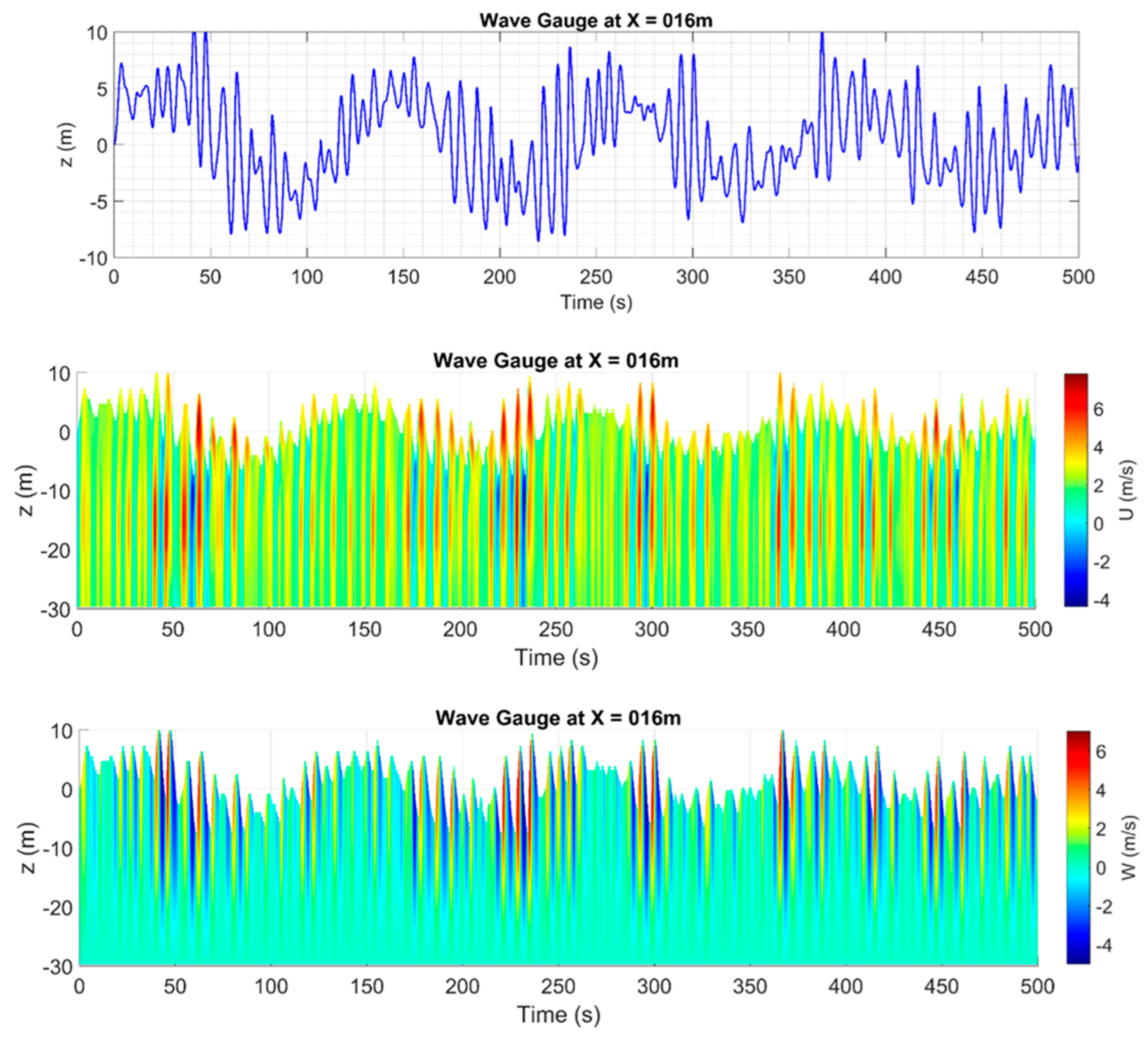
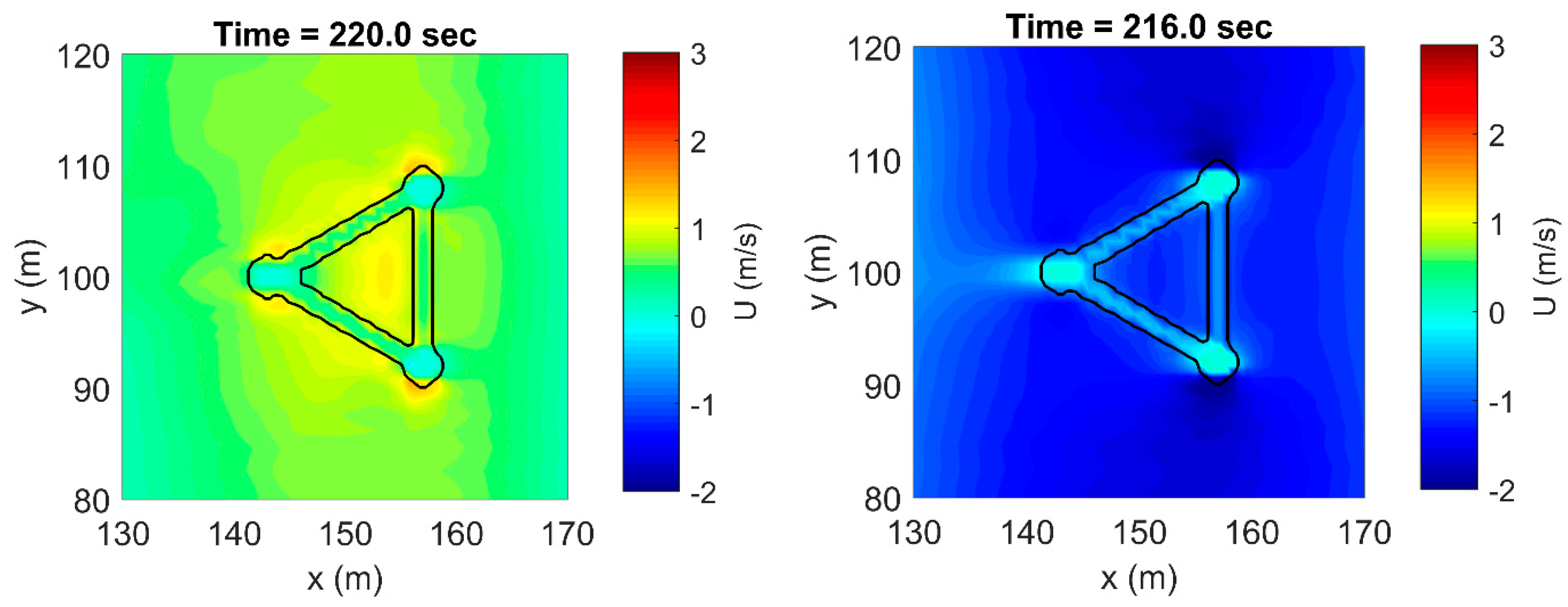
5.1. Case 5-1: Tripod Wind Turbine under Random Waves

Figure 19 shows the maximum negative and positive velocity values near the bottom when the waves pass the tripod wind turbine without current. One interesting thing is that the maximum absolute value of negative velocity is 2.0 m/s, while the maximum absolute value of positive velocity is 2.6 m/s. That causes the local scour downstream of both vertical and horizontal piles, as seen in Figure 20.

In the case of waves, the horseshoe vortex and the lee-wake vortex govern the scouring. These two processes are primarily described by the Keulegan–Carpenter number, KC, which is defined as:

$$KC=\frac{u_m{T}_p}{D}$$

(12)

where $u_m$ is velocity near the bottom, $T_p$ is the peak wave period, and $D$ is the cylinder diameter. When $KC<6$, no horseshoe vortex develops; therefore, no scour hole is formed. The scour hole develops when $KC\ge 6,$ and the empirical formula for the equilibrium scour depth S is [31]:

$$\frac{S}{D}=1.3\left\{1-\exp \left[-0.03\left(KC-6\right)\right]\right\}$$

(13)

In case 5-1, the maximum absolute velocity near the bottom $u_m=2.0 \mathrm{m}/\mathrm{s}$, the peak wave period $T_p=8.0 \mathrm{s}$, and the cylinder diameter $D=3.0 \mathrm{m}$. So, $KC=5.3$. In theory, no scour hole is formed in this case. In the simulation results, we only witness the development of local scour around the horizontal pile downstream.

5.2. Case 5-2: Tripod Wind Turbine under Random Waves and Current

Figure 21 shows the maximum negative and positive velocity values near the bottom when the waves pass the tripod wind turbine in the case with the current. In this case, the random waves are compiled with the current velocity, U = 2.6 m/s. The maximum absolute value of the positive velocity is mildly larger than the maximum absolute value of the negative velocity. The maximum absolute velocity near the bottom is $u_m=2.54 \mathrm{m}/\mathrm{s}$. So, KC = 6.8. The local scour occurs more upstream of both vertical and horizontal piles, as seen in Figure 22. According to the empirical Formula (13), the scour depth is S = 0.089 m (S/D = 0.033).

5.3. Case 5-3: Jack-Up (4-Leg) Wind Turbine under Random Waves

Figure 23 shows the maximum values of negative and positive velocities near the bottom when the waves pass the jack-up wind turbine in the case without current. The maximum absolute value of negative velocity is 2.0 m/s, while the maximum absolute value of positive velocity is 2.6 m/s. That causes the local scour downstream of the piles, as seen in Figure 24.

In cases 5-3, the maximum absolute velocity near the bottom $u_m=2.0 \mathrm{m}/\mathrm{s}$. The KC standard [31] is applied for both regular and irregular waves, according to Equation (12), KC = 5.3. In theory, no scour hole is formed in this case. In the simulation results, however, we can see the signal of scouring development, although the scour depth is shallow.

5.4. Case 5-4: Jack-Up (4-Leg) Wind Turbine under Random Wave—Current

Figure 25 shows the maximum negative and positive velocity values near the bottom when the waves pass the jack-up wind turbine in the case with the current. In this case, the random waves are compiled with the current velocity U = 2.6 m/s; however, the maximum absolute value of the positive velocity is slightly greater than the maximum absolute value of the negative velocity. The local scour occurs more significantly upstream of the piles, as seen in Figure 26.

In cases 5-4, the maximum absolute velocity near the bottom is $u_m=2.7 \mathrm{m}/\mathrm{s}$. So, $KC=7.2$. The local scour occurs more significantly upstream of the vertical piles, as seen in Figure 26. According to the empirical Formula (13), the scour depth is S = 0.138 m (S/D = 0.046).

6. Discussions

This study’s simulation time is only about 200–250 s. The equilibrium state is reached when current passes the monopile wind turbine. The maximum scour depth at the equilibrium state is S/D = 1/6. However, roughly 30–50 waves pass the wind turbine systems for cases of waves. Therefore, the equilibrium state has not been reached in these cases. The maximum scour depth, approximately S/D = 1/12, is only the maximum in the 200–250 s. It is not the maximum local scour at the equilibrium state. In the case of random wave–current coupling, the results present a signal of scour evolution. However, the scour depth is shallow at $0.033\le S/D\le 0.046$.

7. Conclusions

This study uses an in-house code model—Splash3D coupling with a Discontinuous Bi-viscous Model to study the scour phenomena around different wind turbine systems. Local scour under the effect of the current, wave, and wave–current coupling is discussed in this study. Both regular and irregular waves are generated and propagated to the domain using the internal source model. The irregular waves are formed by JONSWAP spectral formulation based on the average spectrum of Taichung Buoy. Three configurations of wind turbines are introduced in this study, including monopile, tripod, and jack-up wind turbines. The results lead to the following important remark points:

• Waves, including regular and irregular waves, do not increase the scour depth compared with currents only.
• The backfilling phenomenon of the scour hole explains the disappearance and reappearance of the local scour in the wave conditions.
• In the case of random wave–current coupling, the results present a signal of scour evolution. However, the scour depth is shallow at $0.033\le S/D\le 0.046$.

References

1. Chen, H.H.; Yang, R.Y.; Hsiao, S.C.; Hwung, H.H. Experimental study of scour around monopile and jacket-type offshore wind turbine foundations. J. Mar. Sci. Technol. 2019, 27, 91–100. [Google Scholar] [CrossRef]
2. Chang, P.C.; Yang, R.Y.; Lai, C.M. Potential of offshore wind energy and extreme wind speed forecasting on the west coast of Taiwan. Energies 2015, 8, 1685–1700. [Google Scholar] [CrossRef]
3. Fang, H.F. Wind energy potential assessment for the offshore areas of Taiwan west coast and Penghu Archipelago. Renew. Energy 2014, 67, 237–241. [Google Scholar] [CrossRef]
4. Igoe, D.; Gavin, K.; O’Kelly, B. An investigation into the use of push-in pile foundations by the offshore wind sector. Int. J. Environ. Stud. 2013, 70, 777–791. [Google Scholar] [CrossRef]
5. Esteban, M.; Lopes-Gutierrez, J.; Diez, J.; Negro, V. Foundations for offshore wind farms. In Proceedings of the 12th International Conference on Environmental Science and Technology, Rhodes, Greece, 8–10 October 2011; pp. 516–523. [Google Scholar]
6. Fischer, T.; De Vries, W.E.; Cordle, A. Executive Summary (WP4: Offshore Foundations and Support Structures), Report—Project Upwind and Integrated Wind Turbine Design, Upwind, TU Delft Publications, Stevinweg, Delft. 2011. Available online: http://resolver.tudelft.nl/uuid:7ff42174-70ab-459d-b709-3bab9c2f9c4b (accessed on 19 April 2023).
7. Frigaard, P.; Hansen, E.A.; Christensen, E.D.; Sand, M. Effect of breaking waves on scour processes around circular offshore wind turbine foundations. In Proceedings of the Copenhagen Offshore Wind Conference & Exhibition, Copenhagen, Denmark, 26–28 October 2005; pp. 1–11. [Google Scholar]
8. Lin, Y.B.; Lin, T.K.; Chang, C.C.; Huang, C.W.; Chen, B.T.; Lai, J.S.; Chang, K.C. Visible light communication system for offshore wind turbine foundation scour early warning monitoring. Water 2019, 11, 1486. [Google Scholar] [CrossRef]
9. Wang, W.-Y.; Yang, J.; Li, R.-Y. Calculation of local scour around wind turbine’s pile of offshore wind farm. J. Waterw. Harb. 2012, 33, 57–60. [Google Scholar]
10. Whitehouse, R.J.S.; Harris, J.; Sutherland, J.; Rees, J. An assessment of field data for scour at offshore wind turbine foundations. In Proceedings of the ICSE 2008 (4th International Conference on Scour and Erosion), Tokyo, Japan, 5–7 November 2008; pp. 1–7. [Google Scholar]
11. Abhinav, K.A.; Saha, N. Effect of scouring in sand on monopile-supported offshore wind turbines. Mar. Georesour. Geotechnol. 2017, 35, 817–828. [Google Scholar] [CrossRef]
12. Harris, J.M.; Whitehouse, R.J.S.; Sutherland, J. Marine Scour and Offshore Wind: Lessons Learnt and Future Challenges. In Proceedings of the International Conference on Offshore Mechanics and Arctic Engineering, Rotterdam, The Netherlands, 19–24 June 2011; Volume 44373, pp. 849–858. [Google Scholar]
13. Liu, P.-F.; Wu, T.-R.; Raichlen, F.; Synolakis, C.E.; Borrero, J.C. Runup and rundown generated by three-dimensional sliding masses. J. Fluid Mech. 2005, 536, 107–144. [Google Scholar] [CrossRef]
14. Wu, T.-R. A Numerical Study of Three-Dimensional Breaking Waves and Turbulence Effects; Cornell University: Ithaca, NY, USA, 2004. [Google Scholar]
15. Hirt, C.W.; Nichols, B.D. Volume of fluid (VOF) method for the dynamics of free boundaries. J. Comput. Phys. 1981, 39, 201–225. [Google Scholar] [CrossRef]
16. Eymard, R.; Gallouët, T.; Herbin, R. Finite volume methods. In Solution of Equation in Rn (Part 3), Techniques of Scientific Computing (Part 3); Elsevier: Amsterdam, The Netherlands, 2000; Volume 7, pp. 713–1018. [Google Scholar]
17. Smagorinsky, J. General circulation experiments wiht the primitive equations I. The basic experiment. Mon. Weather Rev. 1963, 91, 99–164. [Google Scholar] [CrossRef]
18. Vuong, T.-H.-N.; Wu, T.-R.; Wang, C.-Y.; Chu, C.-R. Modeling the slump-type landslide tsunamis part II: Numerical simulation of tsunamis with Bingham landslide model. Appl. Sci. 2020, 10, 6872. [Google Scholar] [CrossRef]
19. Wu, T.-R.; Vuong, T.-H.-N.; Lin, C.-W.; Wang, C.-Y.; Chu, C.-R. Modeling the Slump-Type Landslide Tsunamis Part I: Developing a Three-Dimensional Bingham-Type Landslide Model. Appl. Sci. 2020, 10, 6501. [Google Scholar] [CrossRef]
20. Bingham, E.C. An Investigation of the Laws of Plastic Flow; US Government Printing Office: Washington, DC, USA, 1917.
21. Papanastasiou, T.C. Flows of Materials with Yield. J. Rheol. 1987, 31, 385–404. [Google Scholar] [CrossRef]
22. Beverly, C.R.; Tanner, R.I. Numerical analysis of three-dimensional Bingham plastic flow. J. Nonnewton. Fluid Mech. 1992, 42, 85–115. [Google Scholar] [CrossRef]
23. Jeong, S.W.; Leroueil, S.; Locat, J. Applicability of power law for describing the rheology of soils of different origins and characteristics. Can. Geotech. J. 2009, 46, 1011–1023. [Google Scholar] [CrossRef]
24. Huang, X.; García, M.H. A Herschel-Bulkley model for mud flow down a slope. J. Fluid Mech. 1998, 374, 305–333. [Google Scholar] [CrossRef]
25. Jeong, S.W.; Wu, Y.H.; Cho, Y.C.; Ji, S.W. Flow behavior and mobility of contaminated waste rock materials in the abandoned Imgi mine in Korea. Geomorphology 2018, 301, 79–91. [Google Scholar] [CrossRef]
26. Jeong, S.-W. Shear rate-dependent rheological properties of mine tailings: Determination of dynamic and static yield stresses. Appl. Sci. 2019, 9, 4744. [Google Scholar] [CrossRef]
27. Dean, R.G.; Dalrymple, R.A. Water Wave Mechanics for Engineers and Scientists; World Scientific Publishing Company: Singapore, 1991; Volume 2. [Google Scholar]
28. Baykal, C.; Sumer, B.M.; Fuhrman, D.R.; Jacobsen, N.G.; Fredsøe, J. Numerical simulation of scour and backfilling processes around a circular pile in waves. Coast. Eng. 2017, 122, 87–107. [Google Scholar] [CrossRef]
29. Sumer, B.M.; Petersen, T.U.; Locatelli, L.; Fredsøe, J.; Musumeci, R.E.; Foti, E. Backfilling of a Scour Hole around a Pile in Waves and Current. J. Waterw. Port Coast. Ocean Eng. 2013, 139, 9–23. [Google Scholar] [CrossRef]
30. Hasselmann, K.; Barnett, T.P.; Bouws, E.; Carlson, H.; Cartwright, D.E.; Enke, K.; Ewing, J.A.; Gienapp, A.; Hasselmann, D.E.; Kruseman, P. Measurements of Wind-Wave Growth and Swell Decay during the Joint North Sea Wave Project (JONSWAP), Report—Project Jonswap, Deutches Hydrographisches Institut, TU Delft Publications, Stevinweg, Delft. 1973. Available online: http://resolver.tudelft.nl/uuid:f204e188-13b9-49d8-a6dc-4fb7c20562fc (accessed on 19 April 2023).
31. DNVGL-ST-0126; Support Structures for Wind Turbines. Det Norske Veritas (DNV): Bærum, Norway, 2018.
Figure 1. Comparison between numerical results and analytical solution of the regular wave. The wave solution is the second-order Stokes wave with a wave height of 6 m, wave period of 8 s, and water depth of 30 m; (a) Gauge location at x = 25 m (near the wave maker); (b) Gauge location at x = 105 m (0.83 L).
Jmse 11 00936 g001
Figure 2. (a) Comparison between numerical results and analytical solution of the random wave. The theoretical JONSWAP spectrum (red line) was plotted based on Equation (8). The input wave parameters were taken from buoy data in the Taichung Sea, with a significant wave height of 6 m, peak wave period of 8 s, and water depth of 30 m. The black and blue lines were the JONSWAP spectrum analyzed from the predicted wave at Gauge 1 and 2, respectively. (b) Predicted wave at Gauge 1 (x = 25 m—near the wave maker). (c) Predicted wave at Gauge 2 (x = 105 m).
Jmse 11 00936 g002
Figure 3. Numerical set-up of sand dune morphology analysis (a) Side view; (b) Top view.
Jmse 11 00936 g003
Figure 4. The local scour generation just upstream of the monopile wind turbine under a constant current U = 1.0 m/s.
Jmse 11 00936 g004
Figure 5. A local scour upstream of the monopile wind turbine (top view) at t = 100.1 s. The scour depth is 1.0 m.
Jmse 11 00936 g005
Figure 6. The wave gauges represent the regular wave sent into the domain.
Jmse 11 00936 g006
Figure 7. The mud bed change and the local scour generation around the wind turbine under the regular wave.
Jmse 11 00936 g007
Figure 8. The change of the mud bed and the generation of local scour around the wind turbine under the regular wave and current coupling.
Jmse 11 00936 g008
Figure 9. The local scour downstream of the wind turbine at t = 200.0 s.
Jmse 11 00936 g009
Figure 10. The wave is generated from the average spectrum of Taichung Buoy.
Jmse 11 00936 g010
Figure 11. The mud bed change and local scour generation around the wind turbine under irregular waves.
Jmse 11 00936 g011
Figure 12. The local scour around the wind turbine at t = 220.0 s.
Jmse 11 00936 g012
Figure 13. The mud bed change and the local scour generation around the wind turbine under irregular waves and current coupling.
Jmse 11 00936 g013aJmse 11 00936 g013b
Figure 14. In the case of random waves, water-free surface, horizontal velocity u, and vertical velocity w, the significant wave height Hs = 6.0 m, peak period Tp = 8.0 s.
Jmse 11 00936 g014
Figure 15. In the case of random wave and current, water-free surface, horizontal velocity u, and vertical velocity w, respectively. The significant wave height Hs = 6.0 m, peak period Tp = 8.0 s, and current velocity U = 2.6 m/s.
Jmse 11 00936 g015
Figure 16. Numerical set-up of tripod wind turbine (a) Side view; (b) Top view.
Jmse 11 00936 g016
Figure 17. Numerical set-up of jack-up (4-leg) wind turbine (a) Side view; (b) Top view.
Jmse 11 00936 g017
Figure 18. Topography data were loaded for the mud bottom.
Jmse 11 00936 g018
Figure 19. In this case, the maximum and minimum velocities near the random bottom wave affect the tripod wind turbine.
Jmse 11 00936 g019
Figure 20. The 3D and the top view of the case random wave affecting tripod wind turbine.
Jmse 11 00936 g020
Figure 21. The maximum and minimum velocities near the bottom in the random wave–current affecting the tripod wind turbine.
Jmse 11 00936 g021
Figure 22. The 3D and the top view of the case random wave–current affecting tripod wind turbine.
Jmse 11 00936 g022
Figure 23. The maximum and minimum velocities near the bottom in the case of random waves affecting the jack-up wind turbine.
Jmse 11 00936 g023
Figure 24. The 3D and the top view of the case random waves affected the jack-up wind turbine.
Jmse 11 00936 g024
Figure 25. The maximum and minimum velocities near the bottom in the random wave–current affecting jack-up wind turbine.
Jmse 11 00936 g025
Figure 26. The 3D and the top view of the random wave–current case affecting the jack-up wind turbine.
Jmse 11 00936 g026