Parameter Prediction of the Non-Linear Nomoto Model for Different Ship Loading Conditions Using Support Vector Regression

Abstract

Significant changes in the load of cargo ships make it difficult to simulate and control their motion. In this work, a parameter prediction method for a ship maneuvering motion model is developed based on parameter identification and support vector regression (SVR). First, the effects of least-squares (LS) and multi-innovation least-squares (MILS) parameter identification methods for the non-linear Nomoto model are investigated. The MILS method is then used to identify the parameters of the non-linear Nomoto model under various load conditions, and model training datasets are established. On this basis, SVR is used to predict the parameters of the non-linear Nomoto model. The results reveal that the MILS method converges faster than the LS method. The SVR method achieves lower accuracy than the MILS method, but exhibits reasonable prediction accuracy for zigzag motions, and the maneuvering motion model can be predicted as navigation conditions change.

1. Introduction

In recent years, the impact of economies of scale has led to an increase in ship size, traffic intensity, and related risks [1]. Accurate models for the maneuvering of cargo ships are critical for maneuvering simulations and control applications [2]. Currently, there are three major types of ship maneuvering motion models, the ship hydrodynamics model [3,4], the Maneuvering Modeling Group (MMG) model [5], and the Nomoto model [6]. Although the ship hydrodynamics model and MMG model are of high accuracy, many hydrodynamic parameters are difficult to obtain. The Nomoto model is simple and easy to use, with hydrodynamic parameters that can typically be obtained from captive model tests, numerical calculations based on computational fluid dynamics (CFD), and the system identification method. Captive model tests require expensive towing tanks and numerical calculations consume significant computational resources. The system identification method is practical and effective, and requires little experimental time or cost. This method only needs state information and an inertia term, and does not involve force measurements. As a result, it takes several minutes for a free running test, compared with several weeks for CFD simulations, depending on the propeller modeling and the grid resolution [7]. Thus, it is easier to apply the ship maneuvering model through the system identification method. System identification theory has broad application prospects in ship motion modeling and control, combined with scaled free-running ship models or full-scale ship tests [8]. This theory has been applied in frequency domain identification, Kalman filters (KF), Gaussian process modeling, the maximum likelihood method, neural networks, support vector machines (SVM), least-squares (LS) methods, and hybrid methods. Among these, the LS method is one of the most practical approaches [9]. As an improved recursive form of the LS method, the recursive least-squares (RLS) method has the high identification accuracy and ease-of-use [10], and is widely applied in the identification of ship model parameters.

However, the present work mainly uses a single standard maneuver to generate the training data. For example, Luo et al. [11] used 25${}^{\circ }$/5${}^{\circ }$ zigzag maneuver data as the training set, and predicted the zigzag maneuver motions of 25${}^{\circ }$/5${}^{\circ }$ and 35${}^{\circ }$/5${}^{\circ }$ by SVM and particle swarm optimization (PSO) algorithms. Zhu et al. [12] identified the model parameters by 20${}^{\circ }$/20${}^{\circ }$ zigzag maneuver data using the RLS method based on SVM. Xue et al. [13] used the empirical Bayesian method to clean simulated polluted responses from a 20°/20° zigzag test and identify hydrodynamic parameters. However, the zigzag test datasets for different rudder angles corresponds to different dynamic characteristics. For this reason, scholars such as He et al. [14] used multiple standard maneuver datasets as training data, which ensures a better ability to predict maneuvering motions under a greater range of rudder angles. Wang et al. [15] used the 20${}^{\circ }$/20${}^{\circ }$, 15${}^{\circ }$/15${}^{\circ }$, and 10${}^{\circ }$/10${}^{\circ }$ zigzag test data to cover as many dynamic features as possible. They investigated the fidelity of the model under different levels of perturbation and verified that SVM can achieve better generalization compared to traditional neural networks, but this approach has been validated on constant parameters and cannot be applied to time-varying coefficients. In additional, datasets with different rudder angles are generally used for training without exploring the effect of the rudder angle on the maneuverability parameters, and factors such as ship engine speed, load, and trim are not considered.

For most cargo ships, the load, trim, draft, and engine speed change greatly during daily voyages, making the dynamics characteristics highly variable and leading to uncertainty in maneuverability parameters [16]. More research is required on their effect on maneuverability, which is important for the ease of ship control and safe navigation [17]. If the ship maneuvering motion model cannot be accurately obtained in real-time, the ship’s automatic motion control and autonomous collision avoidance control will be compromised. Ship collisions may lead to devastating consequences, such as a ship capsizing/sinking, resulting in oil spills and fatalities [18]. To solve this problem, Zhang et al. [19] proposed a multi-innovation least-squares (MILS) method for identifying the ship maneuvering model parameters. The MILS method can achieve higher identification accuracy and faster convergence than the RLS method. Wang et al. [20] used non-linear Gaussian filtering algorithm to solve the problem of on-line parameter identification in ship autonomous navigation control. However, during the actual navigation of cargo ships, the ship’s trajectory is mostly straight without larger rudder angles (larger than 10${}^{\circ }$), resulting in insufficient parameter excitation and significant random noise in real-time training data. Thus, the real-time parameter identification method is difficult to generate reasonable results during the actual navigation process that the system identification method is almost useless for cargo ships in a daily voyage. To guarantee a strong excitation of the training data, large yaw-amplitude motions, such as zigzag tests, should be conducted. Unfortunately, it is almost impossible to do so for full-scale ships as the cost is too high. It is a reasonable approach to predict a ship’s motion model in real-time based on groups of identified parameters under several typical operating conditions.

In this study, a scaled free-running ship model is used to perform zigzag tests under different loads, trims, speeds, and rudder angles to obtain the maneuvering motion model of the cargo ship. The non-linear Nomoto model parameters of the scaled free-running ship model under each navigation condition are obtained using the MILS method, and the effects of rudder angle, engine speed, bow trim, stern trim, and load are investigated. SVR is then used to predict the parameters of the non-linear Nomoto model. The prediction accuracy of the Nomoto model parameters is evaluated by comparing the ship motion simulation data with the scaled free-running ship test data. This study makes the following contributions:

(1)

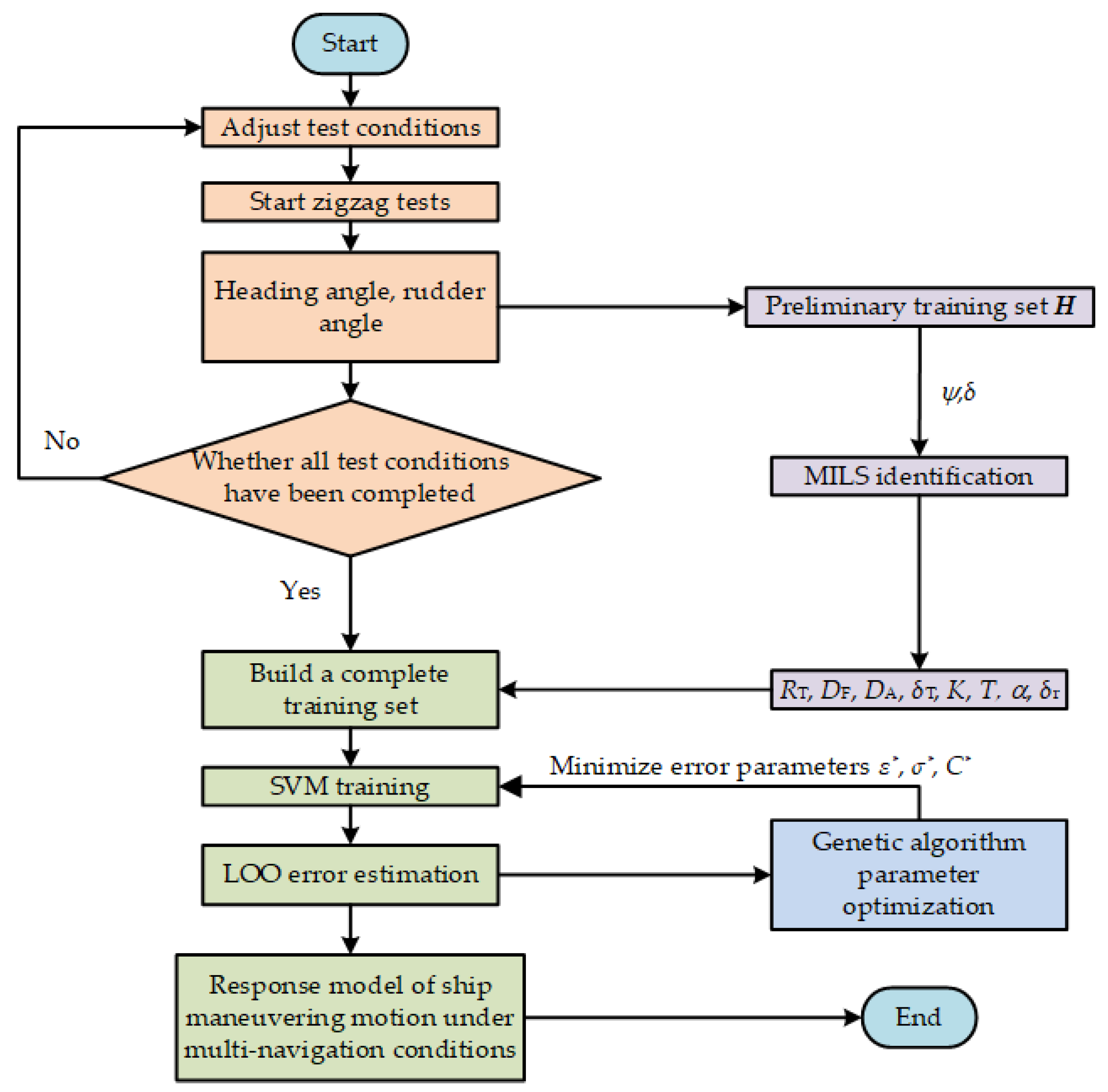
We propose a parameter prediction method for ship maneuvering motion models based on SVR. A training dataset of non-linear Nomoto model parameters under various navigation conditions is established. The proposed algorithm has good prediction accuracy and can quickly obtain the maneuvering model parameters.

(2)

We use the MILS method to identify the parameters of the non-linear Nomoto model under various navigation conditions. Additionally, the effects of rudder angle, engine speed, trim, and load on the maneuvering parameters are analyzed, providing an optimal direction for ship maneuvering and control.

(3)

Based on the parameter identification of the Nomoto model, we include the engine speed, bow and stern draft, and test rudder angle into the training set. The predicted maneuvering motion model can change with navigation conditions, matching the dynamics of the cargo ship in the daily voyage.

2. Parameter Identification of Maneuvering Motion Model

2.1. Ship Maneuvering Motion Model

Considering the balance between model accuracy and calculation efficiency, ship maneuvering motion models are established based on the first-order non-linear Nomoto models. As shown in Figure 1, we take due east as the X-axis and due north as the Y-axis to establish the X–O–Y Earth fixed coordinate system. We take the bow direction as the $x_0$-axis and the starboard direction as the $y_0$-axis to establish the ship’s fixed coordinate system $x_0$–o–$y_0$.

As depicted in Figure 1, $\Psi$ is the ship’s heading angle and r is the yaw angular velocity. Thus, $r=\dot{\psi }$. The first-order non-linear Nomoto model [21] are, respectively, expressed as

$$T\dot{r}+r+\alpha r^3=K(\delta +{\delta }_{\mathrm{r}}),$$

(1)

where K is the turning index; T are time coefficients; ${\delta }_r$ is the effective neutral rudder angle; $\alpha$ is the coefficient of the non-linear term; and $\delta$ is the actual rudder angle. The ship speed in the $x_0$- and $y_0$- directions are u and v, respectively. The ship speed can be expressed as a vector $\mathbf{v}=\left[u,v,r\right]$ and converted to the Earth fixed coordinate system as follows

$$\dot{\mathbf{\eta }}=\mathbf{R}\left(\psi \right)\mathbf{v},$$

(2)

$$\mathbf{R}\left(\psi \right)=\left[\begin{array}{ccc}sin\left(\psi \right)& cos\left(\psi \right)& 0\\ -cos\left(\psi \right)& sin\left(\psi \right)& 0\\ 0& 0& 1\end{array}\right],$$

(3)

where $\mathbf{\eta }$ is the position vector and $\mathbf{R}$$\left(\psi \right)$ is a rotation matrix that maps vectors from a body fixed frame to an inertial frame.

2.2. Model Parameter Identification

2.2.1. Model Discretization

Assuming that the data samples collected from the experiments are discrete with a time step of h, let $y\left(t\right)=\psi \left(t\right)-\psi (t-1)$ and $\dot{\psi }\left(t\right)=\frac{\psi (t+1)-\psi \left(t\right)}{h}$. Then, $\ddot{\psi }\left(t\right)=\frac{y(t+2)-y(t+1)}{h^2}$. With the forward difference quotient used to replace the derivative, Equation (1) can be rewritten as:

$$T\ddot{\psi }\left(t\right)=K(\delta \left(t\right)+{\delta }_r)-\dot{\psi }\left(t\right)-\alpha {\dot{\psi }}^3\left(t\right),$$

(4)

$$y(t+2)-y(t+1)=\frac{K}{T}{h}^2\delta \left(t\right)+\frac{K{\delta }_r}{T}{h}^2-\frac{1}{T}hy(t+1)-\frac{\alpha }{T}\frac{y^3(t+1)}{h},$$

(5)

and

$$y\left(t\right)-y(t-1)=\frac{K}{T}{h}^2\delta (t-2)+\frac{K{\delta }_r}{T}{h}^2-\frac{1}{T}hy(t-1)-\frac{\alpha }{T}\frac{y^3(t-1)}{h}.$$

(6)

Let all parameters be identified as $\mathbf{A}={\left[\begin{array}{cccc}\frac{K}{T}& \frac{K{\delta }_r}{T}& -\frac{1}{T}& -\frac{\alpha }{T}\end{array}\right]}^T$ and all known variables set as $\mathbf{x}\left(t\right)={\left[\begin{array}{cccc}{h}^2\delta (t-2)& h^2& hy(t-1)& \frac{y^3(t-1)}{h}\end{array}\right]}^T$. Then, Equation (6) can be written as:

$$Y\left(t\right)=y\left(t\right)-y(t-1)={\mathbf{x}}^T\left(t\right)·\mathbf{A}.$$

(7)

The left-hand side of Equation (7) is the differences in heading angles. $\mathbf{x}\left(t\right)$ is the information vector and $\mathbf{A}$ is the vector to be identified.

The zigzag maneuver, also known as the Kempf overshoot or “Z” maneuver, is one of the standard test methods for measuring the maneuverability of ships [22]. It is convenient for observation and comparison. Through zigzag tests of the scaled free-running ship model, the heading angle sequences $\mathbf{\psi }\left(t\right)=\left[\psi \left(1\right),\psi \left(2\right),\dots ,\psi \left(t\right)\right]$ and rudder angle sequences $\mathbf{\delta }\left(t\right)=\left[\delta \left(1\right),\delta \left(2\right),\dots ,\delta \left(t\right)\right]$ are obtained. These test data are utilized for identification based on the LS and MILS methods, respectively. The maneuvering motion model parameters (K, T, $\alpha$, and ${\delta }_r$) can then be determined.

2.2.2. Identification Based on LS

It is assumed that the input and output data of the model are sampled from t = 1 to $t=n$, and then the output data $\left\{Y\left(1\right),Y\left(2\right),\dots ,Y\left(n\right)\right\}$ and information data $\left\{\mathbf{x}\left(1\right),\mathbf{x}\left(2\right),\dots ,\mathbf{x}\left(n\right)\right\}$ are obtained. The expanded matrix equations are as follows:

$$\left\{\begin{array}{c}\mathbf{Y}={\mathbf{X}}^T\mathbf{A}\hfill \\ \mathbf{Y}={\left[\begin{array}{cccc}Y\left(n\right)& Y(n-1)& \dots & Y\left(1\right)\end{array}\right]}^T\hfill \\ \mathbf{X}=\left[\begin{array}{cccc}\mathbf{x}\left(n\right)& \mathbf{x}(n-1)& \dots & \mathbf{x}\left(1\right)\end{array}\right]\hfill \end{array}\right..$$

(8)

The LS loss function is expressed as:

$$V_{LS}=\frac{1}{n}\sum _{t=1}^n{(Y\left(t\right)-{\mathbf{x}}^T\left(t\right)\mathbf{A})}^{\mathbf{2}}.$$

(9)

Minimizing the LS loss function gives $\widehat{\mathbf{A}}$, which is the estimated value of $\mathbf{A}$:

$$\widehat{\mathbf{A}}={\left[\mathbf{X}{\mathbf{X}}^T\right]}^{-1}\mathbf{XY}.$$

(10)

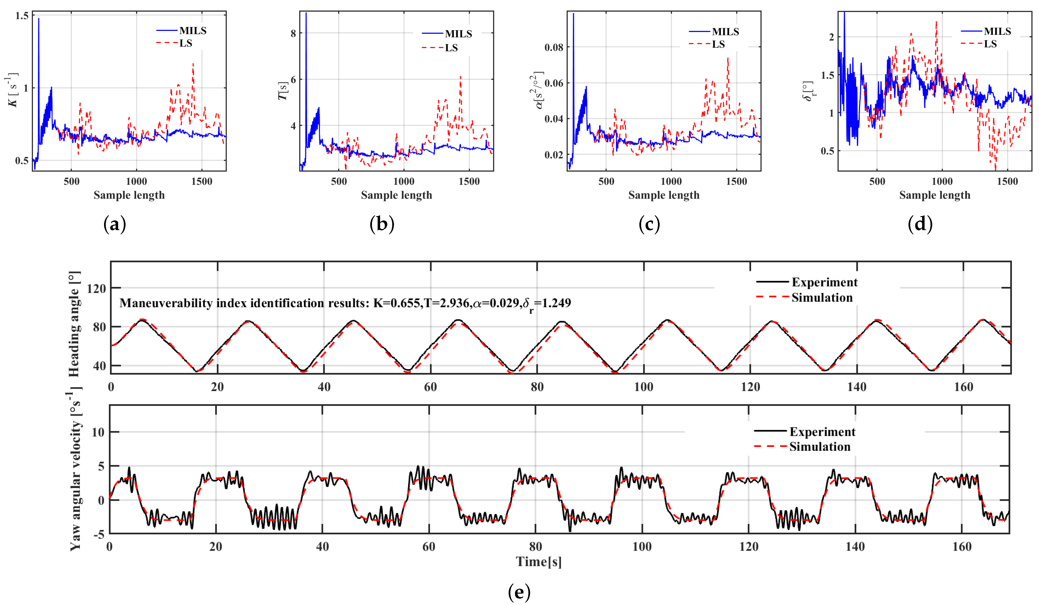
2.2.3. Identification Based on MILS

The recursive equations of the RLS method [23] are

$$\left\{\begin{array}{c}\mathbf{A}\left(t\right)=\mathbf{A}(t-1)+\mathbf{P}\left(t\right)\mathbf{x}\left(t\right)e\left(t\right)\hfill \\ e\left(t\right)=Y\left(t\right)-{\mathbf{x}}^T\left(t\right)\mathbf{A}(t-1)\hfill \\ {\mathbf{P}}^{-1}\left(t\right)={\mathbf{P}}^{-1}(t-1)+\mathbf{x}\left(t\right){\mathbf{x}}^T\left(t\right)\hfill \end{array}\right.,$$

(11)

where $\mathbf{P}\left(t\right)$ is the covariance matrix and $e\left(t\right)$ is the innovation scalar for each iteration. The feature of RLS is that the estimation of parameters in each iteration mainly depends on the current updated information, and past information is generally not used. In real complex navigation conditions, environmental interference often has a negative impact on traditional identification methods. To solve this problem, a multi-innovation identification theory based on an information window with a certain length is proposed [24]. This solves small-sample estimation problems based on the innovation vector. To improve the recognition accuracy by reusing the past state and measurement information, the multi-innovation length p is introduced and the innovation scalar $e\left(t\right)$ is extended to the multi-innovation vector $\mathbf{E}(p,t)$:

$$\mathbf{E}(p,t)=\left[\left.\begin{array}{c}e\left(t\right)\\ e(t-1)\\ ⋮\\ e(t-p+1)\end{array}\right]\right.=\left[\left.\begin{array}{c}Y\left(t\right)-{\mathbf{x}}^T\left(t\right)\mathbf{A}(t-1)\\ Y(t-1)-{\mathbf{x}}^T\left(t\right)\mathbf{A}(t-1)\\ ⋮\\ Y(t-p+1)-{\mathbf{x}}^T(t-p+1)\mathbf{A}(t-1)\end{array}\right]\right..$$

(12)

Similarly, the output vector and information vector of the MILS method are:

$$\left\{\begin{array}{c}\mathbf{Y}(p,t)={\left[\left.\begin{array}{cccc}Y\left(t\right)& Y(t-1)& \cdots & Y(t-p+1)\end{array}\right]\right.}^T\hfill \\ \mathbf{X}(p,t)=\left[\left.\begin{array}{cccc}\mathbf{x}\left(t\right)& \mathbf{x}(t-1)& \cdots & \mathbf{x}(t-p+1)\end{array}\right]\right.\hfill \end{array}\right..$$

(13)

Thus, the recursive equations of the MILS method can be written as:

$$\left\{\begin{array}{c}\mathbf{A}\left(t\right)=\mathbf{A}(t-1)+\mathbf{P}\left(t\right)\mathbf{X}(p,t)\mathbf{E}(p,t)\hfill \\ \mathbf{E}(p,t)=\mathbf{Y}(p,t)-{\mathbf{X}}^T(p,t)\mathbf{A}(t-1)\hfill \\ {\mathbf{P}}^{-1}\left(t\right)={\mathbf{P}}^{-1}(t-1)+\mathbf{X}(p,t){\mathbf{X}}^T(p,t)\hfill \end{array}\right..$$

(14)

3. Parameter Prediction of Maneuvering Motion Model

3.1. Analysis of Navigation Parameters

For cargo ships, the characteristics of the maneuvering motion models will be affected by navigation parameters, such as the ship speed, load, trim, and rudder angle. Considering the detectability, these parameters are simplified as the following.

(1)

Engine speed $R_T$

This study considers a engine that is used to drive the propeller directly, and the engine speed can be accurately measured by the Hall effect element. Thus, the engine speed is indirectly used to reflect the ship speed.

(2)

Bow draft $D_F$ and stern draft $D_A$

The bow and stern draft are used to describe the load and trim of the ship. These quantities can be read from the bow and stern draft scales.

(3)

Test rudder angle ${\delta }_T$

We consider 10${}^{\circ }$/10${}^{\circ }$, 20${}^{\circ }$/20${}^{\circ }$, and 30${}^{\circ }$/30${}^{\circ }$ rudder angles in the zigzag tests. The rudder angle can be measured by an incremental encoder.

Based on the parameter identification of the Nomoto model, the engine speed, bow and stern draft, and test rudder angle are included in the training set for training the SVR model.

3.2. Parameter Training Based on SVR

It is necessary to establish a Nomoto model that can automatically adapt to the navigation conditions. Considering the sample set size, a SVR-based parameter-learning method for the maneuvering motion model is proposed. Let the training sample set be $\left({\mathbf{x}}_i,y_i\right),i=1,2,\dots ,N,{\mathbf{x}}_i\in {\mathbf{R}}^d$, where ${\mathbf{x}}_i$ and $y_i$ denote the input and output spaces, respectively, d is the sample dimension, and N is the number of samples. Then, ${\mathbf{R}}^d$ represents the d-dimensional vector space in which the samples are located. We establish a non-linear mapping from the input space to the output space, $\phi \left(\mathbf{x}\right):{\mathbf{R}}^d\to \mathbf{H}$, and use linear regression to analyze the sample data in the high-dimensional feature space $\mathbf{H}$. The SVR model $f\left(\mathbf{x}\right)=\mathbf{\omega }·\phi \left(\mathbf{x}\right)+b$ can then be established, where $\mathbf{\omega }$ is the weight vector and b is the offset. Introducing the slack variables ${\xi }_i$ and ${\xi }_i^{*}$, the regularized risk function can be transformed into the dual optimization problem,

$$minJ=\frac{1}{2}{∥\mathbf{\omega }∥}^2+C\sum _{i=1}^l\left({\xi }_i+{\xi }_i^{*}\right),$$

(15)

$$\mathrm{subject}\mathrm{to}:\left\{\begin{array}{c}{y}_i-\mathbf{\omega }·\phi \left({\mathbf{x}}_i\right)-b\le \epsilon +{\xi }_i\\ -y_i+\mathbf{\omega }·\phi \left({\mathbf{x}}_i\right)+b\le \epsilon +{\xi }_i^{*}\\ {\xi }_i·{\xi }_i^{*}\ge 0\end{array}\right. i=1,2,\cdots ,l.$$

(16)

where J is the regularized risk, C is the penalty factor, $\epsilon$ is the insensitivity factor, and l is the dimension of the Euclidean space. According to the principle of structural risk minimization, $f\left(x\right)$ should minimize $\frac{\mathrm{N}}{2}{∥\mathbf{\omega }∥}^2$. The weight vector can be expressed as

$$\mathbf{\omega }=\sum _{i=1}^N\left({\lambda }_i-{{\lambda }_i}^{*}\right){\mathbf{x}}_i,$$

(17)

where $\lambda$ is the Lagrange multiplier.

Therefore, the SVR machine can be expressed as:

$$f\left(\mathbf{x}\right)=\sum _{i=1}^N\left({\lambda }_i-{{\lambda }_i}^{*}\right)〈{\mathbf{x}}_i·\mathbf{x}〉+b.$$

(18)

Based on the non-linear characteristics of ship maneuvering motion parameters, the non-linear radial basis function (RBF) kernel is selected as

$$K\left(\mathbf{x},{\mathbf{x}}_i\right)=exp\left\{-\frac{{∥\mathbf{x}-{\mathbf{x}}_i∥}^2}{2{\sigma }^2}\right\},$$

(19)

where $\sigma$ is the parameter of the kernel function.

Although traditional SVR can effectively deal with high-dimensional, non-linear, and small-sample datasets, it is vulnerable to outliers and noise. This is because all samples are treated equally, resulting in a large deviation in the classification interface. A weighted training set based on the sample error is now presented. Based on the parameter identification results of the maneuvering motion model under condition i (described in Section 3.1), the zigzag simulation motion is deduced by using the fourth-order Runge–Kutta (R-K) algorithm to obtain a series of heading angle data. The RMSE between the heading angle simulation and test data are calculated under condition i as:

$$RMS{E}_i(\widehat{\psi },\psi )=\sqrt{\frac{1}{T-1}\sum _{t=0}^T{\left[{\widehat{\psi }}_i\left(t\right)-{\psi }_i\left(t\right)\right]}^2}.$$

(20)

In order to improve the accuracy of RBF-SVR, the influence of training samples with larger identification errors should be weaken. The SVR kernel function is improved by introducing sample weights into the RBF-kernel function.

$$K\left(\mathbf{x},{\mathbf{x}}_i\right)=exp\left\{-\frac{{∥\mathbf{x}-{\mathbf{x}}_i∥}^2}{({\omega }_i+{\omega }_j){\sigma }^2}\right\},$$

(21)

where ${\omega }_i$ is the i-th training sample weight, and ${\omega }_j$ is the j-th test sample weight. These weights are defined as functions of the root mean square error (RMSE) of the training and test samples, as follows:

$${\omega }_i=∥\frac{RMSE{}_i-RMSE{}_{max}-RMSE{}_{min}}{RMSE{}_{max}}∥.$$

(22)

As the main parameters of SVR, $\epsilon$, C, and $\sigma$ have a significant impact on the regression accuracy (i.e., generalization ability) [25]. The leave-one-out (LOO) method is used to investigate the generalization ability of SVR. In the LOO method, one sample is selected as the test set $h\left({\mathbf{x}}_j\right)$, and the remaining samples are used as the training set. SVR is used to obtain the estimated value $\widehat{f}\left({\mathbf{x}}_j\right)$ of the test set. The RMSE of SVR is then used as the precision index:

$$RMSE(\widehat{f},h)=\frac{1}{N-1}\sum _{i=1}^{N-1}\sqrt{\left[\frac{1}{N}\sum _{j=1\mathrm{and}j\ne i}^N{\left(\widehat{f}\left({\mathbf{x}}_j\right)-h\left({\mathbf{x}}_j\right)\right)}^2\right]}.$$

(23)

Taking the minimum RMSE of regression estimation as the optimization goal, the parameters $\epsilon$, C, $\sigma$ are optimized by a genetic algorithm. The fitness value is as follows:

$$fitness=sort\left[1/\phantom{1RMSE\left(\widehat{f},h,\epsilon ,C,\sigma \right)}RMSE\left(\widehat{f},h,\epsilon ,C,\sigma \right)\right].$$

(24)

3.3. Evaluation Indicators

The RMSE and Pearson’s product–moment correlation coefficient (PCC) are used to evaluate the accuracy of the proposed method. The RMSE measures the deviation between the predicted value and the true value, but cannot measure the correlation. Therefore, PCC is used to calculate the correlation between the predicted value and the true value as a supplementary evaluation index. PCC is often denoted as R and is calculated as

$$\overline{h}=\frac{1}{N}\sum _{i=1}^{N}h\left({\mathbf{x}}_j\right),$$

(25)

$$\overline{f}=\frac{1}{N}\sum _{i=1}^N\widehat{f}\left({\mathbf{x}}_j\right),$$

(26)

and

$$R=\frac{{\sum }_{i=1}^N\left.\left\{\left(h\left({\mathbf{x}}_j\right)-\overline{h}\right)\right.\left(\widehat{f}\left({\mathbf{x}}_j\right)-\overline{f}\right)\right\}}{\sqrt{{\sum }_{i=1}^N{\left(h\left({\mathbf{x}}_j\right)-\overline{h}\right)}^2}\sqrt{{\sum }_{i=1}^N{\left(\widehat{f}\left({\mathbf{x}}_j\right)-\overline{f}\right)}^2}}.$$

(27)

4. Test Verification

4.1. Scaled Free-Running Ship Model Test System

The test system is built using the scaled free-running ship model of KVLCC2, as displayed in Figure 2. It is equipped with a main control board, gyrocompass, differential GPS (D-GPS) module (Real-time kinematic, RTK system), rudder angle sensor, and speed sensor, allowing ship motion data to be collected in real-time. The main parameters of the scaled free-running ship model are listed in

Table 1. Parameters of test models.

Parameter	Full-Scale Ship	Scaled Ship Model
Scale ratio	1:1	1:266
Length between perpendiculars ($L_{pp}$)	320 m	1.200 m
Maximum beam of waterline	58 m	0.217 m
Depth	30 m	0.112 m
Draft	20.8 m	0.078 m
Displacement	312,622 t	16.42 kg
Propeller diameter	9.86 m	37 mm
Number of propeller blades	4	4
Propeller area ratio	0.431	0.431
Rudder area	135.9 m${}^2$	0.00192 m${}^2$
Rudder turning rate	2.34${}^{\circ }$/s	38.24${}^{\circ }$/s

, and more details of KVLCC2 can be found on SIMMAN 2014 [26].

4.2. Test Conditions

To obtain the navigation data of the ship model, the zigzag test conditions are set in terms of the engine speed, test rudder angle, and bow and stern draft, as depicted in

Table 2. Zigzag test conditions.

Navigation Condition	Engine Speed (rpm)	Bow Draft (cm)	Stern Draft (cm)	Test Rudder Angle (${}^{\circ }$)
Light load	2000	7	7	10${}^{\circ }$/10${}^{\circ }$ 20${}^{\circ }$/20${}^{\circ }$ 30${}^{\circ }$/30${}^{\circ }$
	3000	7	7
Full load	2000	9	9
	3000	9	9
Bow trim	2000	7	5
	3000	7	5
Stern trim	2000	5	7
	3000	5	7

. It should be noted that the light load mentioned is relative to the full load. Bow and stern trim are a lighter condition than the light load. To ensure that the rotational inertia moment of the ship model remains unchanged in each repeated test, the bow and stern draft are adjusted by uniformly pasting ballast lead blocks at fixed positions along the length of the ship. We set the rudder turning rate of the full-scale ship as ${\omega }_{\mathrm{S}}$, the scale ratio of the model as $R_{\mathrm{S}}$, and the rudder turning rate of the scaled model as ${\omega }_{\mathrm{M}}={\omega }_{\mathrm{S}}·\sqrt{R_{\mathrm{S}}}$. This ensures that the angular velocity of the rudder is similar to that of the full-scale ship.

4.3. Test Data Analysis

4.3.1. Parameter Identification

The free-running model tests were carried out in a lake, as displayed in Figure 3. The heading angle $\psi \left(t\right)$ and rudder angle $\delta \left(t\right)$ of the scaled free-running ship model were recorded with a frequency of 10 Hz to form a preliminary training set $\mathbf{H}\left(t\right)=\left[\psi \right(t\left)\delta \right(t\left)\right]$. To study the convergence of the identification parameters, the preliminary training set was split into a series of training samples according to the time length, and parameter identification based on the LS method was carried out. Meanwhile, considering data convergence and computational efficiency [23], the innovation length was set to 4, and parameter identification based on the MILS method was performed. Taking the navigation condition of a 2000 rpm engine speed, 20${}^{\circ }$ rudder angle, 5 cm bow draft, and 7 cm stern draft as an example, Figure 4 reveals the parameter identification results of the first-order non-linear Nomoto models.

As depicted in Figure 4a–d, for the first-order non-linear Nomoto model, the MILS method converges faster than the LS method. The parameters K, T, and $\alpha$ converge after approximately 500 iterations (i.e., 50 s). The effective neutral rudder angle ${\delta }_r$ converges relatively slowly, requiring around 1500 iterations. This is because low-frequency random disturbances (e.g., randomness of ship motion) influence the scaled free-running ship model as it sails. The fourth-order R-K integration method was used to simulate the motion of the ship model, and the heading angle and yaw angular velocity are shown in Figure 4e. From Figure 4e, the simulation heading angles are very similar to the experimental data. In the remainder of this study, the MILS method is used to identify the parameters of the first-order non-linear Nomoto model. This allows us to analyze the law of the maneuvering motion model parameters under different navigation conditions.

4.3.2. Parameter Training

A series of zigzag tests were carried out under the navigation conditions listed in Table 2. The first-order non-linear Nomoto model parameters were identified by the MILS method. At least five zigzag tests should be carried out under each navigation condition. Due to the deviation of the results obtained in each identification, the parameters of the maneuvering motion model are shown as box diagrams in Figure 5 and Figure 6, where 7-5 represents the bow trim condition, 5-7 represents the stern trim condition, 7-7 represents the light load condition, and 9-9 represents the full load condition. Under four test conditions (1: rudder angle 30${}^{\circ }$, bow trim, engine speed 2000 rpm; 2: rudder angle 10${}^{\circ }$, bow trim, engine speed 3000 rpm; 3: rudder angle 30${}^{\circ }$, bow trim, engine speed 3000 rpm; and 4: rudder angle 30${}^{\circ }$, full load, engine speed 3000 rpm), many experimental data are invalid and unstable due to the random environmental disturbances, non-linear ship motion, the data collection process, and other factors. Thus, only one grouping of valid data are identified.

The test rudder angle ${\delta }_T$, rudder force $F_{\delta }$, rudder force arm $A_{\delta }$, ship turning inertia $I_{zz}$, hydrodynamic force $F_W$, and hydrodynamic action area of the underwater hull $S_h$ have significant impacts on the maneuvering performance. As shown in Figure 5 and Figure 6, under the same engine speed and rudder angle conditions, K and T are greater under the bow trim condition than under the stern trim condition, and are greater under the full load condition than under the light load condition. In general, $I_{zz}$ and $F_{\delta }$ are very similar in the bow trim (7-5) and stern trim (5-7) conditions; however, $A_{\delta }$ is larger in the bow trim condition, and so K and T are greater in the bow trim condition than in the stern trim condition. Compared with the light load condition (7-7), $S_h$ is larger in the full load condition (9-9), resulting in a larger value of $I_{zz}$. Thus, K is larger in the full load condition, which means that the turning angular velocity is higher. Because of the larger $I_{zz}$, the value of T in the full load condition is higher than in the light load condition, meaning that it takes longer to enter the stable turning state. The values of K and T basically decrease with increasing rudder angle. A change in rudder angle usually causes the ship to turn and change its course, which will affect the speed and turning rate of the ship. Within a certain range of rudder angles, the ship’s steering response accelerates as the rudder angle increases, but this also enhances the ship’s lateral resistance, reducing the driving force and steering ability of the ship; thus, K and T decrease accordingly. Note that an excessive rudder angle not only increases the ship’s navigation resistance, but also aggravates the ship’s sway and affects the ship’s stability. Comparing Figure 5a with Figure 6a and Figure 5b with Figure 6b, it is clear that a higher speed produces a larger value of K and a lower value of T. The reason may be that the higher speed increases the rudder force and turning torque, enhancing the turning rate.

From Figure 5c, $\alpha$ approaches zero as the rudder angle increases, meaning that a larger rudder angle decreases the non-linear motion. This may be because the hydrodynamic forces and moments are sufficiently large at greater rudder angles, while the random disturbances are not significant; however, this phenomenon does not occur at an engine speed of 3000 rpm. The effective neutral rudder angle ${\delta }_r$ exhibits strong randomness in different conditions, making it difficult to determine the change rule and hydrodynamic action mechanism. ${\delta }_r$ is the angle of a ship’s rudder necessary to maintain its heading with no lateral force applied. It is affected by the ship speed, draft, and environmental interference. There is no obvious regularity in the change of ${\delta }_r$. Fortunately, the influence of ${\delta }_r$ is limited.

The first-order non-linear Nomoto model parameters identified by MILS and the engine speeds, bow and stern drafts, and test rudder angles of the scaled free-running ship model were non-dimensionalized and normalized to create a complete training set: ${\mathbf{G}}_i=[R_{Ti},D_{Fi},D_{Ai},{\delta }_{Ti},K_i,T_i,{\alpha }_i,{\delta }_{ri}]$. SVR training was used to obtain rapid regression predictions of the ship maneuvering motion parameters under any condition. The specific process is illustrated in Figure 7. Additionally,

Table 3. The optimal kernel function parameters.

Nomoto Model Parameters	Kernel Function Parameters of SVR
	$\mathbf{\epsilon }$	$\mathit{C}$	$\mathbf{\sigma }$
K (s${}^{-1}$)	0.000002	0.86	1.175
T (s)	0.001	2.561	0.922
a (s/${}^{\circ }$${}^2$)	0.000001	0.156	0.021
${\delta }_r$ (${}^{\circ }$)	0.00002	4.0103	1.041

shows the optimal kernel function parameters.

4.4. Model Accuracy Verification

We used the MILS method to directly identify the parameters of the first-order non-linear Nomoto model, and compared them with the SVR prediction results, as illustrated in

Table 4. Comparison of identified results.

Verification Condition	Navigation Condition Parameters				K (s${}^{-1}$)		T (s)		a (s/${}^{\circ }$${}^2$)		${\mathit{\delta }}_{\mathit{r}}$ (${}^{\circ }$)
	Engine Speed (rpm)	Rudder Angle (${}^{\circ }$)	Bow Draft (cm)	Stern Draft (cm)	MILS	SVR	MILS	SVR	MILS	SVR	MILS	SVR
1	2000	15	8	8	0.559	0.566	4.282	4.009	−0.004	0.0094	0.492	0.620
2	2500	25	6	8	0.415	0.430	1.228	1.303	0.023	0.0076	2.013	2.419

. Under the two verification conditions, the values of K and T predicted by the SVR are close to those directly identified by the MILS, although the effective neutral rudder angle ${\delta }_r$ is slightly different. The variation of the non-linear coefficient $\alpha$ is relatively large. In addition, it can be seen from the analysis in Section 4.3.2 that K and T decrease as the rudder angle increases. K and T decrease in stern trim conditions. Additionally, K and T increase with increasing load, while a higher engine speed lead to a higher K value and lower T value. The coupling effect of rudder angle, load, stern trim, and engine speed makes the reduction in K less than the reduction in T.

The parameters obtained by the MILS and SVR methods were used for dynamic simulations. To further validate the method proposed in this study, the computational results of the MMG parameters of KVLCC2 by Yasukawa et al. [27] were cited and compared with the simulation results by numerical integration of the differential equation, as shown

Table 5. Hydrodynamic derivatives used in the simulations [27,28].

Surge Force Derivatives		Lateral Force Derivatives		Yaw Moment Derivatives
$R_0{}^{\prime }$	0.022	$Y_v{}^{\prime }$	−0.315	$N_v{}^{\prime }$	−0.137
$X_{vv}{}^{\prime }$	−0.040	$Y_r{}^{\prime }$	0.083	$N_r{}^{\prime }$	−0.049
$X_{vr}{}^{\prime }$	0.002	$Y_{vvv}{}^{\prime }$	−1.607	$N_{vvv}{}^{\prime }$	−0.030
$X_{rr}{}^{\prime }$	0.011	$Y_{vvr}{}^{\prime }$	0.379	$N_{vvr}{}^{\prime }$	−0.294
$X_{vvvv}{}^{\prime }$	0.771	$Y_{vrr}{}^{\prime }$	−0.391	$N_{vrr}{}^{\prime }$	0.055
		$Y_{rrr}$	0.008	$N_{rr}{}^{\prime }$	−0.013

. Where the primary figure input to the symbol means a non-dimensionalized value, force and moment are non-dimensionalized by $1/2\rho L_{pp}d{U}^2$ and $1/2\rho L_{pp}^{2}d{U}^2$, respectively. More details can be found in the references [27,28]. It is worth noting that the shape of the blades was modified due to the difficulty of machining the prototype propeller. The simulated and experimental results of the zigzag motions are shown in Figure 8. The SVR and MILS results in condition 2 are close to the experimental data, while the MMG results have a phase lead compared with the experimental data. In condition 1, the SVR and MMG results have a phase lag compared with the experimental data and MILS results.

Table 6. Comparison of overshoot angles.

Verification Condition	Overshoot Angle	Test (${}^{\circ }$)	MILS (${}^{\circ }$)	SVR (${}^{\circ }$)	MMG (${}^{\circ }$)
1	1st overshoot	12.17	7.89	7.51	10.71
	2nd overshoot	13.62	11.7	8.97	12.31
2	1st overshoot	12.03	8.97	7.75	16.88
	2nd overshoot	12.04	8.13	6.62	14.96

compares the overshoot angles in the zigzag maneuvers. The overshoot angles of the SVR and MILS simulation results are smaller than the experimental values. The overshoot angle of MMG simulation results is less than the experimental value in condition 1 and greater than the experimental value in condition 2. In condition 1, the MMG method is more accurate in predicting overshoot angles, while, in condition 2, it has comparable accuracy to MILS. It is difficult to predict the overshoot angle to within a few degrees [27]. The RMSE and PCC between the simulated and experimental heading angles are listed in

Table 7. Simulated and experimental error statistics of zigzag motions.

Verification Condition	Method	RMSE (${}^{\circ }$)	PCC
1	MILS	3.8414	0.9839
	SVR	5.9296	0.9639
	MMG	5.3710	0.9725
2	MILS	4.8138	0.9847
	SVR	6.2458	0.9733
	MMG	7.1617	0.9638

. The errors and correlation coefficients of the MILS simulation results are better than SVR and MMG. This is because the MILS method is a direct identification, using information from the current navigation condition for identification. The method based on SVR is an indirect identification; it does not use data from the current navigation condition, but trains the MILS identification results of other navigation conditions to predict the current value. The hydrodynamic derivatives of MMG were obtained based on captive tests of a 2.902 m model ship. There is a scale effect with the ship model in this study. In general, however, the RMSE and PCC values are reasonable under the verification conditions, indicating that the SVR-based prediction method proposed in this study has good generalization ability.

5. Conclusions and Prospects

Based on the parameter identification of the Nomoto model, the SVR method has been used to predict the parameters of ship maneuvering. Using a desktop computer (Intel^® Core™ i7-10700F CPU @2.90 GHz, 40 GB RAM), the average training time of the SVR model was just 1.5 s. The scaled free-running ship model experiments show that the proposed method has good prediction accuracy and can quickly obtain the maneuvering model parameters. The specific conclusions are the following.

(1)

The MILS and LS methods have good accuracy for parameter identification with the first-order non-linear Nomoto models. In general, the MILS method converges faster than the LS method. Thus, the MILS method was used to identify the parameters of the first-order Nomoto model with different maneuvering motions. The resulting dataset was trained using the SVR-based method to predict 15${}^{\circ }$/15${}^{\circ }$ and 25${}^{\circ }$/25${}^{\circ }$ zigzag motions. The results show that the SVR-based prediction method can obtain the Nomoto model parameters quickly, although the accuracy is slightly lower than that of the MILS method.

(2)

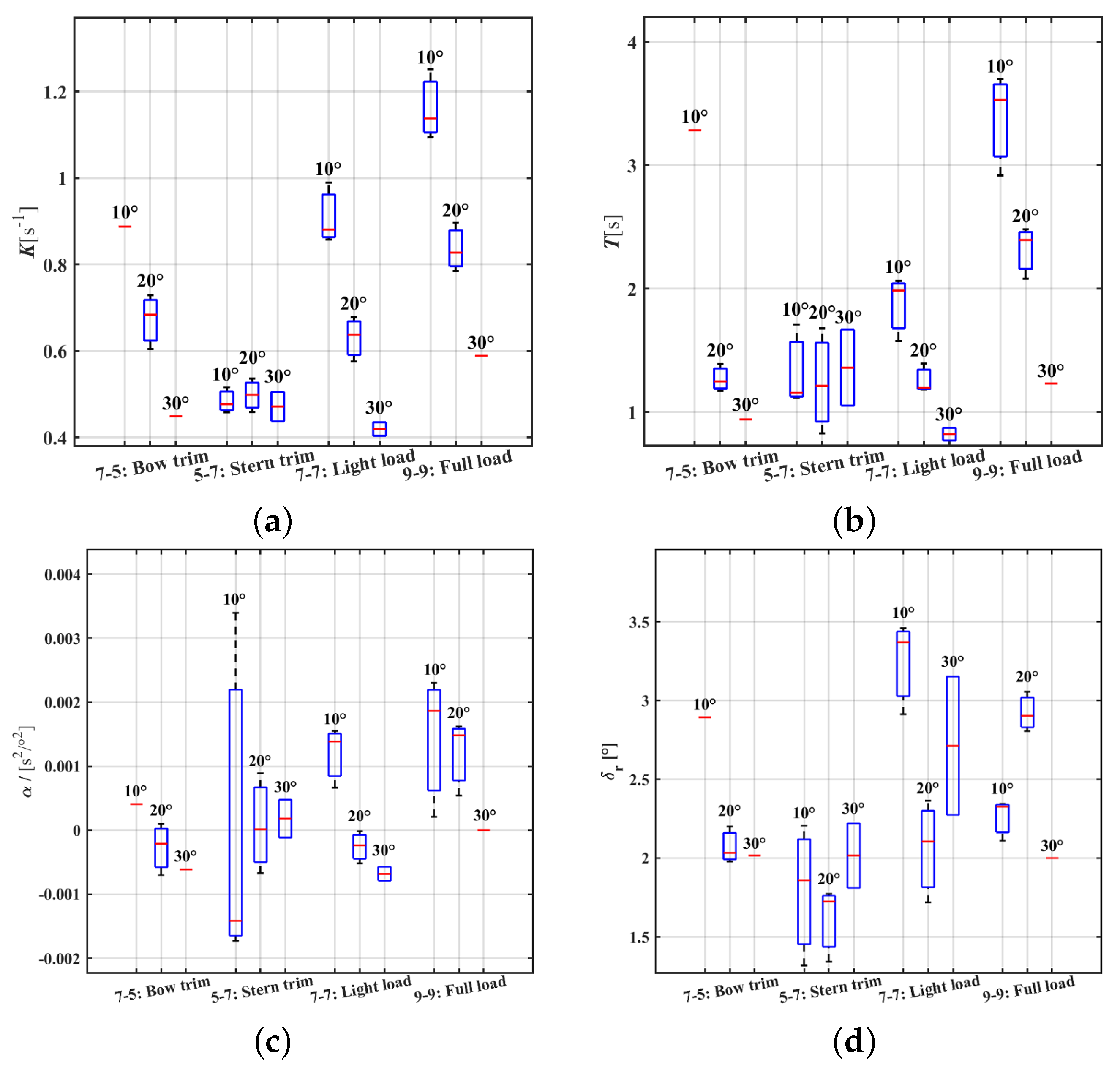
The effects of rudder angle, engine speed, bow trim, stern trim, and load on the maneuvering coefficients were analyzed. K and T are larger in the bow trim condition than in the stern trim condition. In the full load condition, K and T are larger. K and T decrease as the rudder angle increases. Additionally, higher speeds lead to higher K values and lower T values. At an engine speed of 2000 rpm, $\alpha$ approaches zero as the rudder angle increases; however, this does not occur at an engine speed of 3000 rpm. The effective neutral rudder angle ${\delta }_r$ exhibits strong randomness under different conditions, making it difficult to determine the variation pattern of this parameter and its hydrodynamic action mechanism.

This study has presented a method for solving the problem of insufficient excitation of cargo ship navigation data. By considering the influence of engine speed, load, trim, and rudder angle, the ship motion model under various load conditions in a daily voyage can be predicted. The main limitations of the proposed method are that the accuracy is slightly lower than that of the direct identification method (e.g., MILS), and large amounts of historical data of various navigation conditions are required for training. Although we have tried our best to understand and explain the hydrodynamics, it may be flawed in some aspects. In addition, the SVR model is trained based on zigzag experimental data and can only be used for zigzag-like maneuvers of ships. However, zigzag maneuvers seem not to be fully representative for anti-collision or track-change maneuvers in open sea. In future work, there should be a better balance between zigzag and turning circle tests in those fields of ship operations.

References

1. Zhang, M.; Kujala, P.; Hirdaris, S. A machine learning method for the evaluation of ship grounding risk in real operational conditions. Reliab. Eng. Syst. Saf. 2022, 226, 108697. [Google Scholar] [CrossRef]
2. Zhang, M.; Taimuri, G.; Zhang, J.; Hirdaris, S. A deep learning method for the prediction of 6-DoF ship motions in real conditions. Proc. Inst. Mech. Eng. Part M J. Eng. Marit. Environ. 2023; online first. [Google Scholar] [CrossRef]
3. Abkowitz, M.A. Lectures on Ship Hydrodynamics–Steering and Manoeuvrability; Technical Report Hy-5; Hydro-and Aerodynamic Laboratory: Lyngby, Denmark, 1964. [Google Scholar]
4. Norrbin, N.H. Theory and Observations on the Use of a Mathematical Model for Ship Manoeuvring in Deep and Confined Waters; Publication 68 of the Swedish State Shipbuilding Experimental Tank, Göteborg, Sweden. In Proceedings of the 8th Symposium on Naval Hydrodynamics, ONR, Pasadena, CA, USA, 24–28 August 1971; pp. E807–E905. [Google Scholar]
5. Ogawa, A.; Kasai, H. On the mathematical model of manoeuvring motion of ships. Int. Shipbuild. Prog. 1978, 25, 306–319. [Google Scholar] [CrossRef]
6. Nomoto, K.; Taguchi, K.; Honda, K.; Hirano, S. On the steering qualities of ships. J. Zosen Kiokai 1956, 1956, 75–82. [Google Scholar] [CrossRef] [PubMed]
7. Araki, M.; Sadat-Hosseini, H.; Sanada, Y.; Tanimoto, K.; Umeda, N.; Stern, F. Estimating maneuvering coefficients using system identification methods with experimental, system-based, and CFD free-running trial data. Ocean Eng. 2012, 51, 63–84. [Google Scholar] [CrossRef]
8. Carrillo, S.; Contreras, J. Obtaining first and second order Nomoto models of a fluvial support patrol using identification techniques. Ship Sci. Technol. 2018, 11, 19–28. [Google Scholar] [CrossRef]
9. Xu, H.; Hinostroza, M.; Soares, C.G. Estimation of hydrodynamic coefficients of a nonlinear manoeuvring mathematical model with free-running ship model tests. Int. J. Marit. Eng. 2018, 160, A3. [Google Scholar] [CrossRef]
10. Caccia, M.; Indiveri, G.; Veruggio, G. Modeling and identification of open-frame variable configuration unmanned underwater vehicles. IEEE J. Ocean. Eng. 2000, 25, 227–240. [Google Scholar] [CrossRef]
11. Luo, W.; Guedes Soares, C.; Zou, Z. Parameter identification of ship maneuvering model based on support vector machines and particle swarm optimization. J. Offshore Mech. Arct. Eng. 2016, 138, 031101. [Google Scholar] [CrossRef]
12. Zhu, M.; Hahn, A.; Wen, Y.; Bolles, A. Parameter identification of ship maneuvering models using recursive least square method based on support vector machines. TransNav Int. J. Mar. Navig. Saf. Sea Transp. 2017, 11, 23–29. [Google Scholar] [CrossRef]
13. Xue, Y.; Liu, Y.; Ji, C.; Xue, G. Hydrodynamic parameter identification for ship manoeuvring mathematical models using a Bayesian approach. Ocean Eng. 2020, 195, 106612. [Google Scholar] [CrossRef]
14. He, H.W.; Zou, Z.J. Black-box modeling of ship maneuvering motion using system identification method based on BP neural network. In Proceedings of the International Conference on Offshore Mechanics and Arctic Engineering, Virtual, 3–7 August 2020; Volume 84386, p. V06BT06A037. [Google Scholar]
15. Wang, T.; Li, G.; Wu, B.; Æsøy, V.; Zhang, H. Parameter identification of ship manoeuvring model under disturbance using support vector machine method. Ships Offshore Struct. 2021, 16, 13–21. [Google Scholar] [CrossRef]
16. Borkowski, P. Inference engine in an intelligent ship course-keeping system. Comput. Intell. Neurosci. 2017, 2017, 2561383. [Google Scholar] [CrossRef] [PubMed]
17. Himaya, A.N.; Sano, M.; Suzuki, T.; Shirai, M.; Hirata, N.; Matsuda, A.; Yasukawa, H. Effect of the loading conditions on the maneuverability of a container ship. Ocean Eng. 2022, 247, 109964. [Google Scholar] [CrossRef]
18. Zhang, M.; Conti, F.; Le Sourne, H.; Vassalos, D.; Kujala, P.; Lindroth, D.; Hirdaris, S. A method for the direct assessment of ship collision damage and flooding risk in real conditions. Ocean Eng. 2021, 237, 109605. [Google Scholar] [CrossRef]
19. Huajun, Z.; Xinchi, T.; Hang, G.; Shou, X. The parameter identification of the autonomous underwater vehicle based on multi-innovation least squares identification algorithm. Int. J. Adv. Robot. Syst. 2020, 17, 1729881420921016. [Google Scholar] [CrossRef]
20. Wang, S.; Wang, L.; Im, N.; Zhang, W.; Li, X. Real-time parameter identification of ship maneuvering response model based on nonlinear Gaussian Filter. Ocean Eng. 2022, 247, 110471. [Google Scholar] [CrossRef]
21. Tzeng, C.Y.; Chen, J.F. Fundamental properties of linear ship steering dynamic models. J. Mar. Sci. Technol. 2009, 7, 2. [Google Scholar] [CrossRef]
22. Hinostroza, M.; Xu, H.; Guedes Soares, C. Experimental and Numerical Simulations of Zig-Zag Manoeuvres of a Self-Running Ship Model; Taylor & Francis Group: London, UK, 2017; pp. E563–E570. [Google Scholar]
23. Xie, S.; Chu, X.; Liu, C.; Liu, J.; Mou, J. Parameter identification of ship motion model based on multi-innovation methods. J. Mar. Sci. Technol. 2020, 25, 162–184. [Google Scholar] [CrossRef]
24. Zhao, B.; Zhang, X.; Liang, C. A Novel Parameter Identification Algorithm for 3-DOF Ship Maneuvering Modelling Using Nonlinear Multi-Innovation. J. Mar. Sci. Eng. 2022, 10, 581. [Google Scholar] [CrossRef]
25. Cherkassky, V.; Ma, Y. Practical selection of SVM parameters and noise estimation for SVM regression. Neural Netw. 2004, 17, 113–126. [Google Scholar] [CrossRef]
26. Simman. Workshop on Verification and Validation of Ship Manoeuvring Simulation Methods. 2014. Available online: http://simman2014.dk (accessed on 1 March 2022).
27. Yasukawa, H.; Yoshimura, Y. Introduction of MMG standard method for ship maneuvering predictions. J. Mar. Sci. Technol. 2015, 20, 37–52. [Google Scholar] [CrossRef]
28. Yoshimura, Y.; Ueno, M.; Tsukada, Y. Analysis of steady hydrodynamic force components and prediction of manoeuvring ship motion with KVLCC1, KVLCC2 and KCS. In Proceedings of the Workshop Proceedings of SIMMAN2008, Copenhagen, Denmark, 7 April 2008; Volume 1, pp. E80–E86. [Google Scholar]
Figure 1. Coordinate system of ship maneuvering motion.
Jmse 11 00903 g001
Figure 2. Ship maneuverability test platform. (a) Scaled free-running ship model. (b) Shipboard control terminal. (c) Major sensors and controllers on board.
Jmse 11 00903 g002
Figure 3. Zigzag tests.
Jmse 11 00903 g003
Figure 4. Results of the first-order non-linear Nomoto model. (a) Convergence process of K. (b) Convergence process of T. (c) Convergence process of α . (d) Convergence process of δ r . (e) Time history of heading angle and yaw angular velocity for experimental and simulated data.
Jmse 11 00903 g004
Figure 5. Identification results at 2000 rpm engine speed. (a) Identification results of K. (b) Identification results of T. (c) Identification results of α . (d) Identification results of δ r .
Jmse 11 00903 g005
Figure 6. Identification results at 3000 rpm engine speed. (a) Identification results of K. (b) Identification results of T. (c) Identification results of α . (d) Identification results of δ r .
Jmse 11 00903 g006
Figure 7. Flowchart of ship maneuvering motion model under multi-navigation conditions.
Jmse 11 00903 g007
Figure 8. Simulated and experimental results of zigzag motions. (a) Comparison of results under verification condition 1. (b) Comparison of results under verification condition 2.
Jmse 11 00903 g008