Numerical Analysis of Energy Loss in Stall Zone for Full Tubular Pump Based on Entropy Generation Theory

Abstract

As a low-head and non-drive pump, the head reduction and stall advance are the key factors that restrict the popularization and application of the full tubular pump (FTP). In this paper, the shear stress transport (SST) k-ω turbulence model is used for the numerical calculation of the FTP. Additionally, based on the entropy generation theory, the energy loss and main distribution zones of the FTP under all working conditions are analyzed, and the mechanism of inducing its stall advance is explored. By comparison, we found that there is little difference between the numerical simulation results and the model test. Turbulence entropy generation has a high proportion under small flow conditions, which is mainly reflected in the outlet flow separation zone of the suction surface of the impeller blade, the guide vane inlet zone where inlet deviation exists, and the trailing edge of the guide vane where the flow separation exists. Compared with the axial flow pump (AFP), when the flow rate decreases, the clearance reflow between the stator and rotor induces the deterioration of the flow at the impeller inlet, and the turbulent entropy generation in the impeller channel increases rapidly, making the FTP enter the stall zone ahead of time. The clearance backflow affects the flow pattern of the inlet pipe, making the turbulence entropy generation in the outlet area of the inlet pipe increase. The total entropy generation in the stator–rotor region is little affected by the pump flow conditions, and it is mainly affected by different stator–rotor backflow clearance dimensions. This study can provide a reference for exploring the energy loss of the FTP and revealing its stall characteristics.

1. Introduction

In today’s economic development, energy utilization is an inevitable topic. As a new type of non-drive and low-head pump, the full tubular pump (FTP) has a simple structure and is easy to install. Compared with traditional pumps, it can save project investment and has better application in hydraulic conservancy projects [1,2]. As the impeller of the FTP is directly arranged inside the motor rotor, the motor and pump are integrated. However, the clearance between the stator and rotor causes backflow to affect the inlet flow field of the FTP [3,4,5]. At the same time, compared with the conventional axial flow pump (AFP), the performance curve has a more obvious saddle zone. To accurately analyze the cause and distribution of the dissipation of the FTP, the traditional pressure drop method only analyzes the total loss value of a certain calculation zone from a macro perspective, and cannot directly reflect the large loss value of a certain region. Therefore, this paper uses the entropy generation analysis method [6,7,8], which can quantitatively analyze the dissipation to specifically analyze what causes the increase in FTP dissipation and exacerbates the stall phenomenon of the FTP under small flow conditions.

Because the entropy generation theory is intuitionistic, many scholars use the entropy generation theory to analyze the dissipation of hydraulic machinery. Shen et al. [9,10] used the entropy generation theory to analyze the energy dissipation of the AFP and found that the impeller is the main zone of energy dissipation. The energy dissipation of the impeller is closely related to the characteristics of the saddle zone. Zhang et al. [11] analyzed the energy loss of AFP reverse power generation and found that, due to the lack of guide vane rectification during AFP reverse operation, the entropy generation of the outlet channel was high, so it is necessary to optimize the outlet channel during power generation operation. Yang et al. [12,13] used entropy generation to analyze the energy loss of the AFP as a turbine and found that flow separation and reflow were the main reasons for high entropy generation. Pei et al. [14] analyzed the influence of the distance between the impeller and the guide vane on the performance of the two-way tubular pump, and found that the change in the distance did not significantly affect the turbulence dissipation in the impeller, but it did affect the turbulence dissipation in the guide vane. Kan et al. [15,16] analyzed the energy conversion relationship between the pump condition and the turbine condition of the AFP, and found that the total entropy generation of the forward transition was greater than the reverse one. The tip leakage flow affected the hydraulic efficiency of the turbine. Yu et al. [17] analyzed the energy characteristics of the turbine and found that most of the energy loss in the runner was concentrated in the channel near the lower ring. Meng et al. [18] analyzed the mechanical energy characteristics of the two-way AFP compared to two impellers, and found that the total entropy generation distribution of the arc and S-shaped impellers was similar, and the total entropy generation under the reverse condition mainly came from the impeller and the straight pipe. Li et al. [19] analyzed the effect of AFP root clearance size on mechanical energy and found that the flow pattern at the impeller was affected by the leakage of the root clearance, and the indirect dissipation and total dissipation rate of the impeller increased with the increase in the root clearance. Li et al. [20] analyzed the saddle zone characteristics of the turbine based on entropy generation theory and found that the saddle zone characteristics were caused by the loss of the runner and fixed guide vane. Chang et al. [21] analyzed the size and location of energy loss of self-priming pumps with different blade thicknesses based on entropy generation theory, and found that the hydraulic performance of blades with increasing blade thickness was better than that with decreasing blade thickness.

According to previous studies, this paper uses the entropy generation theory to analyze the flow field in an FTP, explore the composition, size, and location of FTP energy loss, and explore the induction reason for the stall zone of the FTP. This study can provide a reference for exploring the energy loss and stall characteristics of the FTP [22,23,24].

2. Numerical Simulation

2.1. Control Equation and Turbulence Model

It was assumed that the fluid density inside the FTP is constant. The Reynolds time-average N-S equation was used to control the calculation model, as shown in Equations (1) and (2).

$$\frac{\partial \rho }{\partial \mathrm{t}}+\frac{\partial }{\partial x_i}\left(\rho u_i\right)=0$$

(1)

$$\frac{\partial }{\partial \mathrm{t}}\left(\rho u_i\right)+\frac{\partial }{\partial x_j}\left(\rho u_i{u}_j\right)=-\frac{\partial p}{\partial x_j}+\frac{\partial }{\partial x_j}\left(\mu \frac{\partial u_i}{\partial x_j}-\rho \overline{{u^{\prime }}_i{u^{\prime }}_j}\right)+S_i$$

(2)

where ρ is the density; t is the physical time; x_i and x_j represent the Cartesian coordinate components in the i and j directions, respectively; u_i and u_j represent the corresponding components of the time-averaged velocity; p is the local pressure; m is the dynamic viscosity; and S_i is the Reynolds stress.

The SST k-ω turbulence model was chosen to close the equation and obtain effective solutions. The model is a two-equation model, which takes into account the turbulent shear force in the counter pressure boundary layer so as to better predict the flow separation [25,26,27]. In addition, the prediction equation can be converted near the wall and the main flow zone to predict the viscosity characteristics near the impeller of the FTP and the rotor wall of the motor more accurately. The specific formulas are (3)–(5).

$$\frac{\partial \left(\rho k\right)}{\partial \mathrm{t}}+\frac{\partial \left(\rho U_{j}k\right)}{\partial x_j}=P_k-\beta \ast \rho k\omega +\frac{\partial }{\partial x_j}\left[\left(\mu +\frac{{\mu }_t}{{\sigma }_{k1}}\right)\frac{\partial k}{\partial x_j}\right]$$

(3)

$$\frac{\partial \left(\rho \omega \right)}{\partial \mathrm{t}}+\frac{\partial \left(\rho U_j\omega \right)}{\partial x_j}=\frac{\partial }{\partial x_j}\left[\left(\mu +\frac{{\mu }_t}{{\sigma }_{\omega 1}}\right)\frac{\partial \omega }{\partial x_j}\right]+{\alpha }_1\frac{\omega }{k}{P}_k-{\beta }_1\rho {\omega }^2+2\left(1-F_1\right)\rho {\sigma }_{\omega 2}\frac{1}{\omega }\frac{\partial k}{\partial x_j}\frac{\partial \omega }{\partial x_j}$$

(4)

$$P_k={\mu }_t\left(\frac{\partial u_i}{\partial x_j}+\frac{\partial u_j}{\partial x_i}\right)\frac{\partial u_i}{\partial x_j}-\frac{2}{3}\left(\rho k+{\mu }_t\frac{\partial u_i}{\partial x_i}\right)\frac{\partial u_k}{\partial x_k}$$

(5)

where k is the turbulent kinetic energy (m²/s²), ω is the turbulent eddy frequency (s⁻¹), U_j is the velocity vector, and P_k is the generation rate of turbulence. The model constants are given by: β = 0.09, α₁ = 5/9, β₁ = 0.075, σ_k1 = 2, and σ_ω1 = 2.

2.2. Entropy Generation Theory

Entropy describes the degree of disorder of the system. The second law of thermodynamics describes that the loss of mechanical energy becomes internal energy, and eventually leads to an increase in entropy. In the operation of fluid machinery, water is considered an incompressible constant temperature (25 °C) medium. Due to the viscosity of the fluid, part of the kinetic energy and pressure energy generated by impeller rotation is converted into internal energy. Therefore, the entropy generation theory can be used to analyze energy loss in fluid machinery. The fluid velocity in turbulent motion is composed of average velocity and fluctuating velocity [28], so the entropy generation (S_E) of the fluid includes two parts:

$$S_E=S_{DE}+S_{TE}$$

(6)

In the post-processing of the numerical simulation, the direct entropy generation caused by uneven average velocity can be obtained, but the entropy generation caused by fluctuating velocity cannot be obtained. Following studies by Koch [29,30] and Herwig [31], the unavailable S_TE was converted to be related to the k-ε formula.

$$S_{TE}=\frac{\rho \epsilon }{T}$$

(7)

For the SST k-ω turbulence model used in this paper, the turbulent entropy generation caused by the fluctuating velocity can be replaced by the following equation:

$$S_{TE}=\alpha \frac{\rho \omega k}{T}$$

(8)

Among them, α is the empirical constant, α = 0.09; ω is the turbulent eddy frequency (s⁻¹); and k is the turbulent kinetic energy (m²/s²).

In addition, in the near wall region of the fluid machinery, there is a higher velocity gradient, which leads to higher wall entropy generation. Therefore, (11) was used to calculate the wall entropy generation (S_WE) in this study:

$$S_{WE}=\frac{\tau \cdot v}{T}$$

(9)

where τ is the wall shear force (Pa) and v is the velocity (m/s) of the first layer mesh node of the wall.

By integrating the entropy generation rate per unit fluid volume and per unit zone, different types of entropy generation can be obtained [32], including direct entropy generation, turbulent entropy generation and wall entropy generation, as follows: (10)–(12):

$$\Delta S_{pro,DE}={\displaystyle {\int }_V{S}_{DE}dV}$$

(10)

$$\Delta S_{pro,TE}={\displaystyle {\int }_V{S}_{TE}dV}$$

(11)

$$\Delta S_{pro,WE}={\displaystyle {\int }_A{S}_{WE}dA}$$

(12)

V is the volume of FTP(m³) and A is the wall area of FTP(m²).

Finally, the total entropy generation (ΔS_pro) of the whole flow channel in the flow process is as follows (13):

$$\Delta S_{pro}=\Delta S_{pro,DE}+\Delta S_{pro,TE}+\Delta S_{pro,WE}$$

(13)

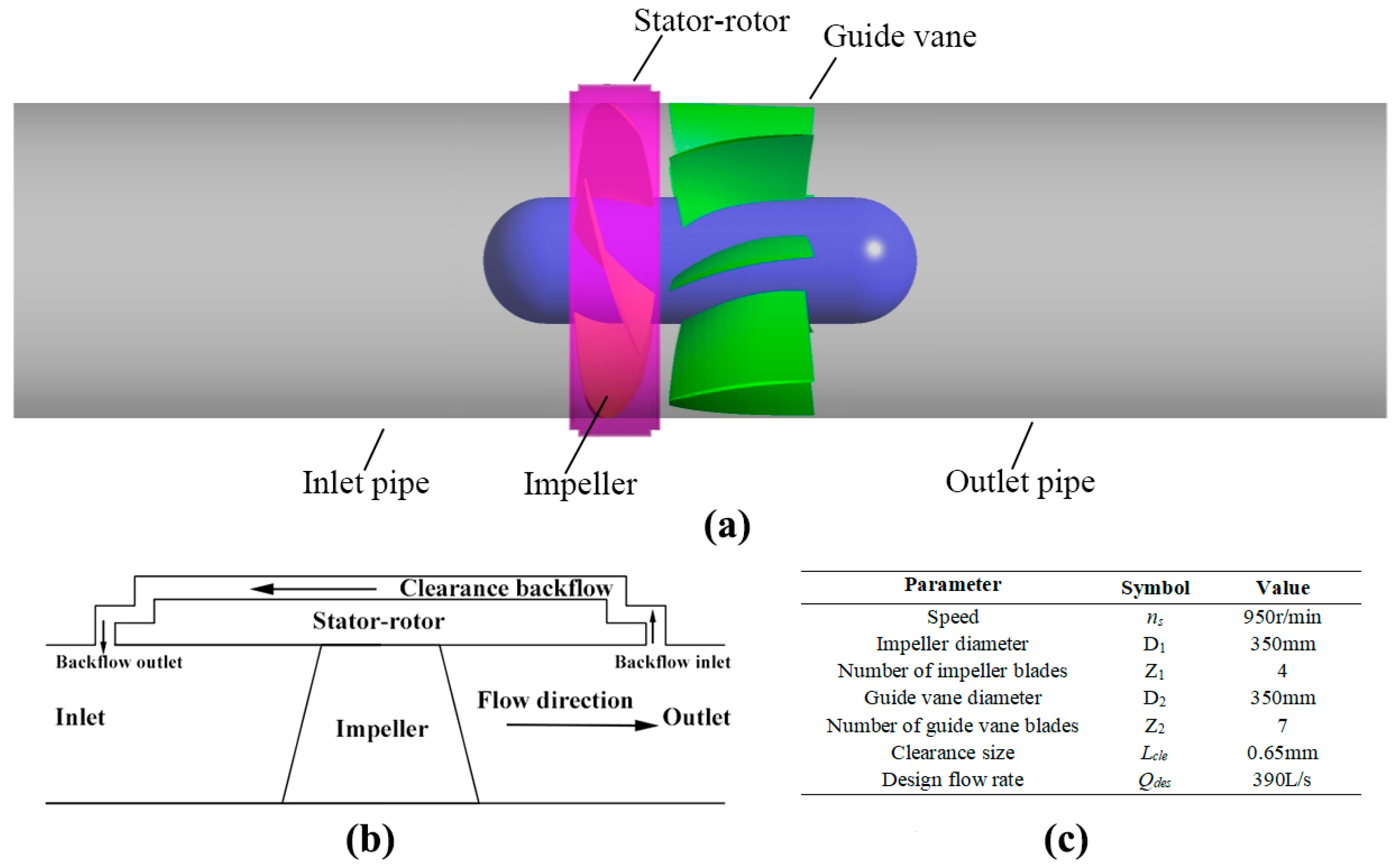
2.3. Three-Dimensional Simulation Model

Figure 1a shows the FTP used in this simulation, which is primarily composed of five flow components: inlet pipe, impeller, stator–rotor (motor rotor), guide vane, and outlet pipe. Figure 1b shows the flow diagram in the impeller chamber when the FTP is running. It can be found that the clearance backflow between the stator and rotor is directly connected to the impeller chamber. Because of the pressure difference between the inlet and outlet of the impeller, there is backflow through the clearance of the stator–rotor. The smaller the flow, the greater the pressure difference, and the greater the clearance backflow. The clearance backflow can cool the motor, but because it flows from the impeller inlet side perpendicular to the flow direction of the main flow, the clearance backflow interacts with the impeller inlet flow field to interfere with the flow pattern of the impeller chamber. Throughout the entire computational domain, the impeller and rotor in the stator–rotor are relatively stationary. Figure 1c shows the main characteristic parameters of the FTP; the impeller diameter D₁ is 350 mm, the number of blades Z₁ is 4, the hub ratio of the blades is 0.4, and the nD value is 332.5. The guide vane diameter D₂ is 350 mm, the number of blades Z₂ is 7, and the hub ratio of the guide vane is 0.4. The clearance at the stator–rotor is 0.65 mm, the speed n_s is 950 r/min, and the design flow rate is 390 L/s.

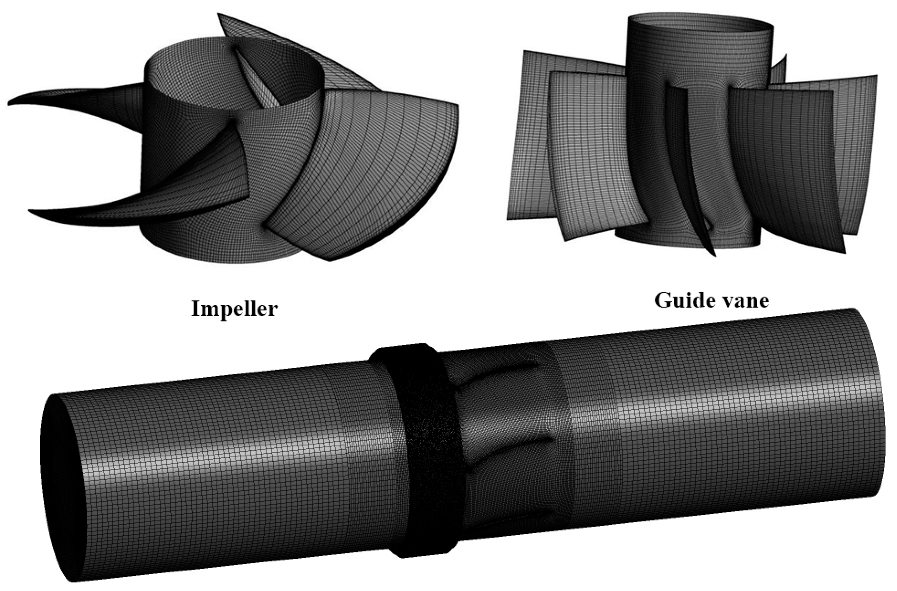
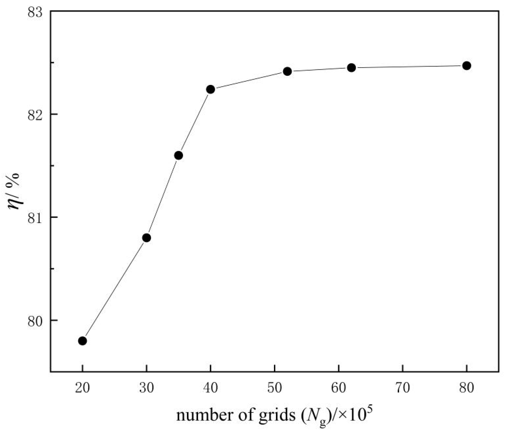
2.4. Computational Grid and Grid-Independent Analysis

The simulation model was meshed based on Ansys Turbogrid and ICEM, and the FTP was generated by the hybrid grid. The inlet pipe and outlet pipe generated structured grids in ICEM, the stator–rotor generated unstructured grids, and the impeller and guide vane generated structured grids in Turbogrid. Figure 2 shows the grid figure of the FTP model. The grid length–width ratio is strictly controlled between 10 and 100 to ensure the impact of the grid quality on the FTP numerical simulation. At 1.0 Qdes, the y+ values of different flow components of the FTP are as follows: the y+ value in the inlet pipe is about 258, the y+ value in the impeller is about 26, the y+ value in the guide vane is about 55, and the y+ value in the outlet pipe is about 233. The y+ values meet the requirements of the numerical simulation. The efficiency of the FTP was chosen as the monitoring parameter of the grid-independent analysis in the numerical simulation. Figure 3 shows the effect of different grid numbers on the FTP efficiency. After the grid number reached 3.96 million, the efficiency change value was not obvious, and the efficiency increased by 0.23%, from 3.96 million grids to 8 million grids. In order to facilitate calculation and save calculation resources [33,34], 3.96 million grids were finally selected for the further numerical calculation of the FTP.

2.5. Boundary Condition Settings

This numerical simulation was carried out in Ansys CFX. The impeller and motor rotor were set as the rotating domain, while the other domains were set as the static domain. The coupling between the rotating domain and the static domain adopted the frozen rotor method, and the transient frozen rotor slip interface was used for information transmission between the rotating domain and the static domain. The inlet of the inlet pipe was set as the total pressure inlet, the outlet of the outlet pipe was set as the mass flow outlet, and the wall of all flow channel components was set as a smooth wall without slip. The convergence residual was set to 10⁻⁶, and the calculation step was 1500.

3. Model Test

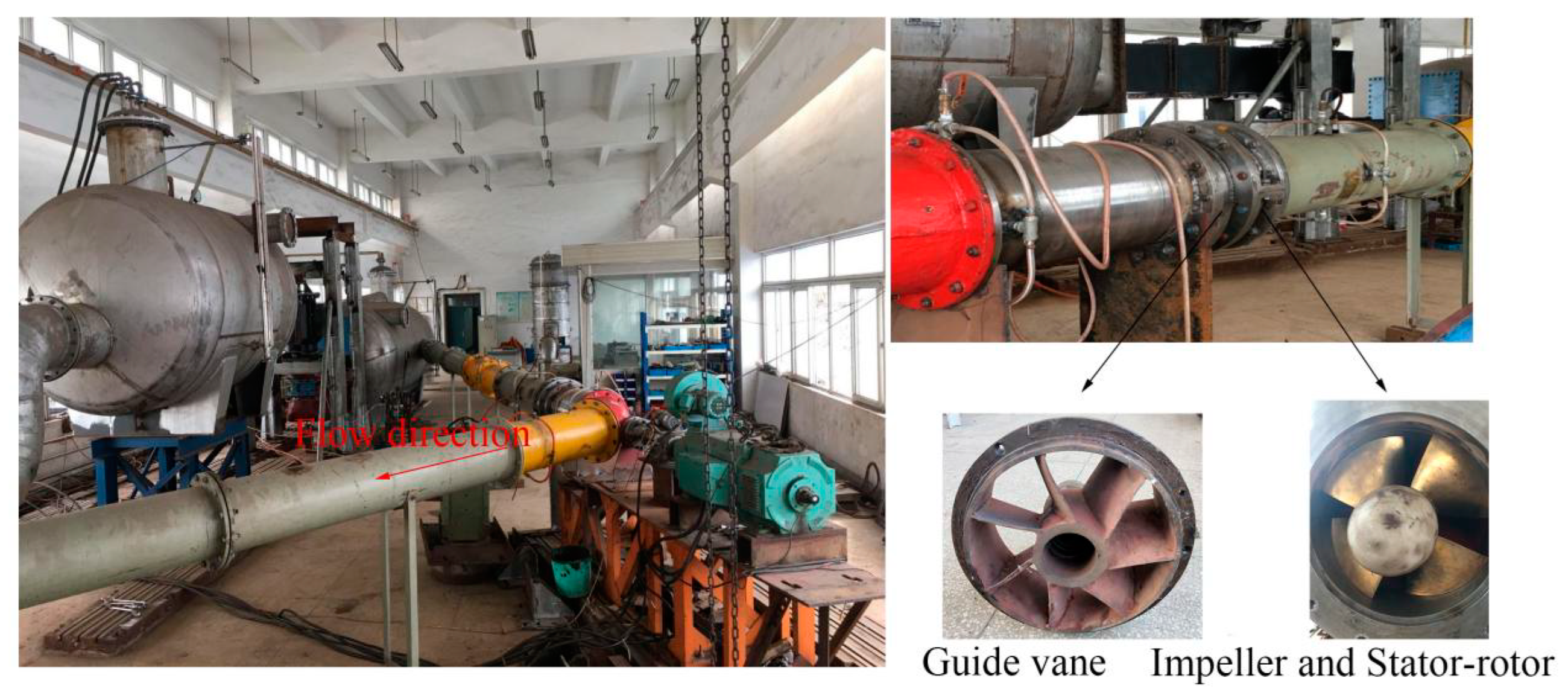
3.1. Description of Testing Instruments

The model test of the FTP device was carried out on a high-precision test bench.

Table 1. Main equipment parameters.

Test Equipment	Model	Operating Value	Uncertainty
Differential pressure transmitter	EJA10A	0~200 kpa	±0.1%
Electromagnetic flow meter	E-mag	DN400mm	±0.2%
Speed torque sensor	ZJ	500 N·m	±0.15%

shows the parameters of the main instruments for this test. The sensors used in this test bench meet the inspection requirements [35,36]. The test uncertainty was higher than the requirements in SL140~2006. The physical model is shown in Figure 4.

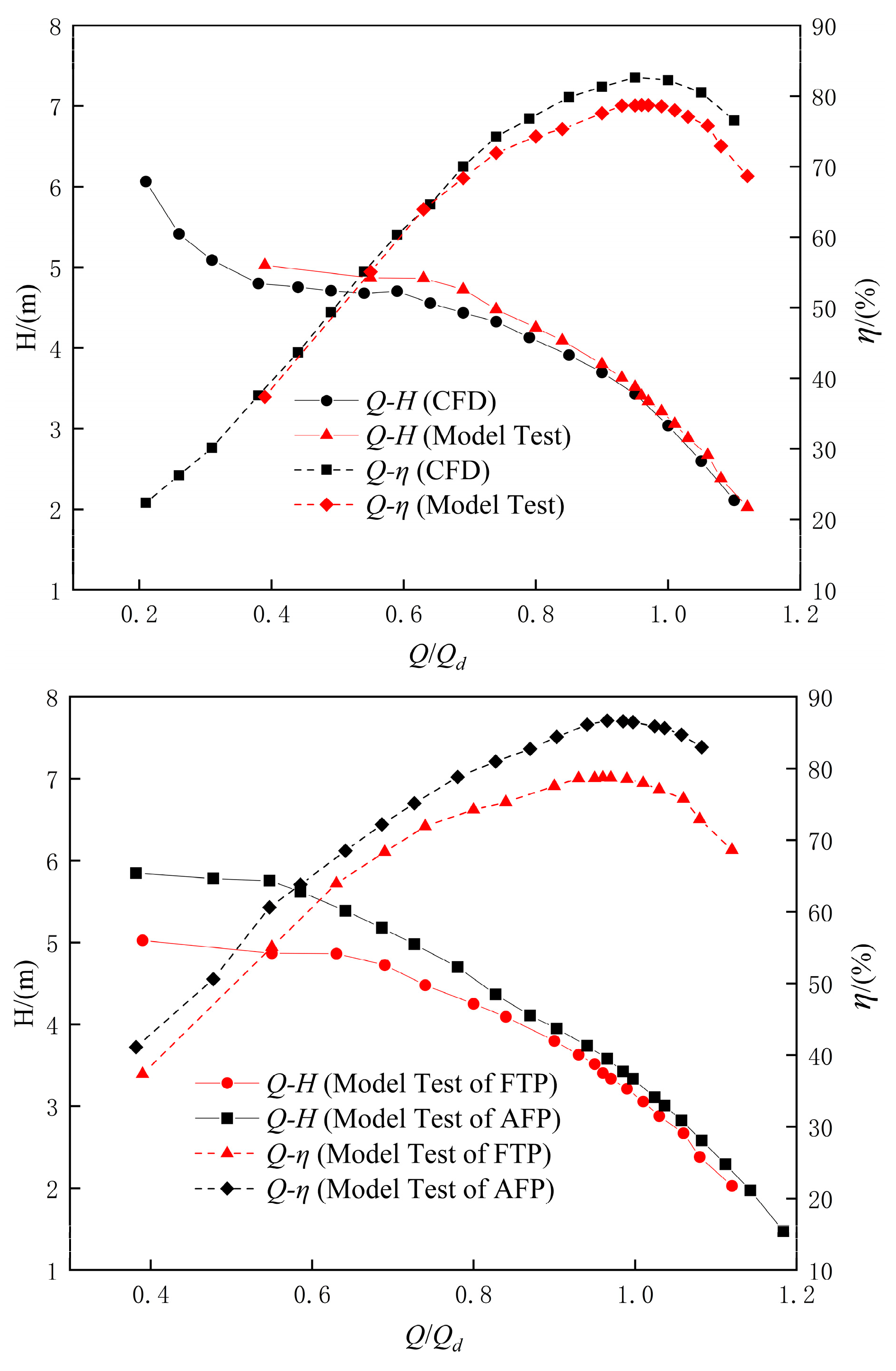
3.2. Numerical Simulation Verification

Through the external characteristic test of the FTP and the conventional AFP on the test bench, the experimental data at the blade placement angle of 0° were selected to compare them with the results of the numerical simulation. The comparison results are shown in Figure 5. It was found that the changing trend in the numerical simulation curve of the FTP device model was basically consistent with that of the test curve. When operating in an efficient FTP range, the flow–head curve of the experiment and numerical simulation fit well, but the efficiency had some errors. At 1.0 Q_des, the efficiency of the FTP obtained by experiment was 78.83%, and the efficiency of the FTP obtained by numerical simulation was 82.24%, with an error of 3.41%, which is within the calculation error. Under small flow conditions, the flow–efficiency curve of the experiment and numerical simulation fit well. There was an error in the flow–head curve of the two. The maximum error was around 0.6 Q_des. Under this condition, the head of the FTP obtained from the experiment was 4.867 m, and the head of the FTP obtained from the numerical simulation was 4.573 m, with an error of 0.294 m. The comparison of the external characteristics between the experiment and the numerical simulation proves that the numerical simulation was effective and reliable.

According to the experimental comparison between the FTP and the AFP in Figure 5, the flow–head of the FTP has a long stall zone under small flow conditions, that is, the zone where the head increases slowly. In order to describe the size and distribution of the energy loss in the stall zone more vividly, the entropy generation theory is used to analyze the energy loss of the FTP.

4. Results and Analysis

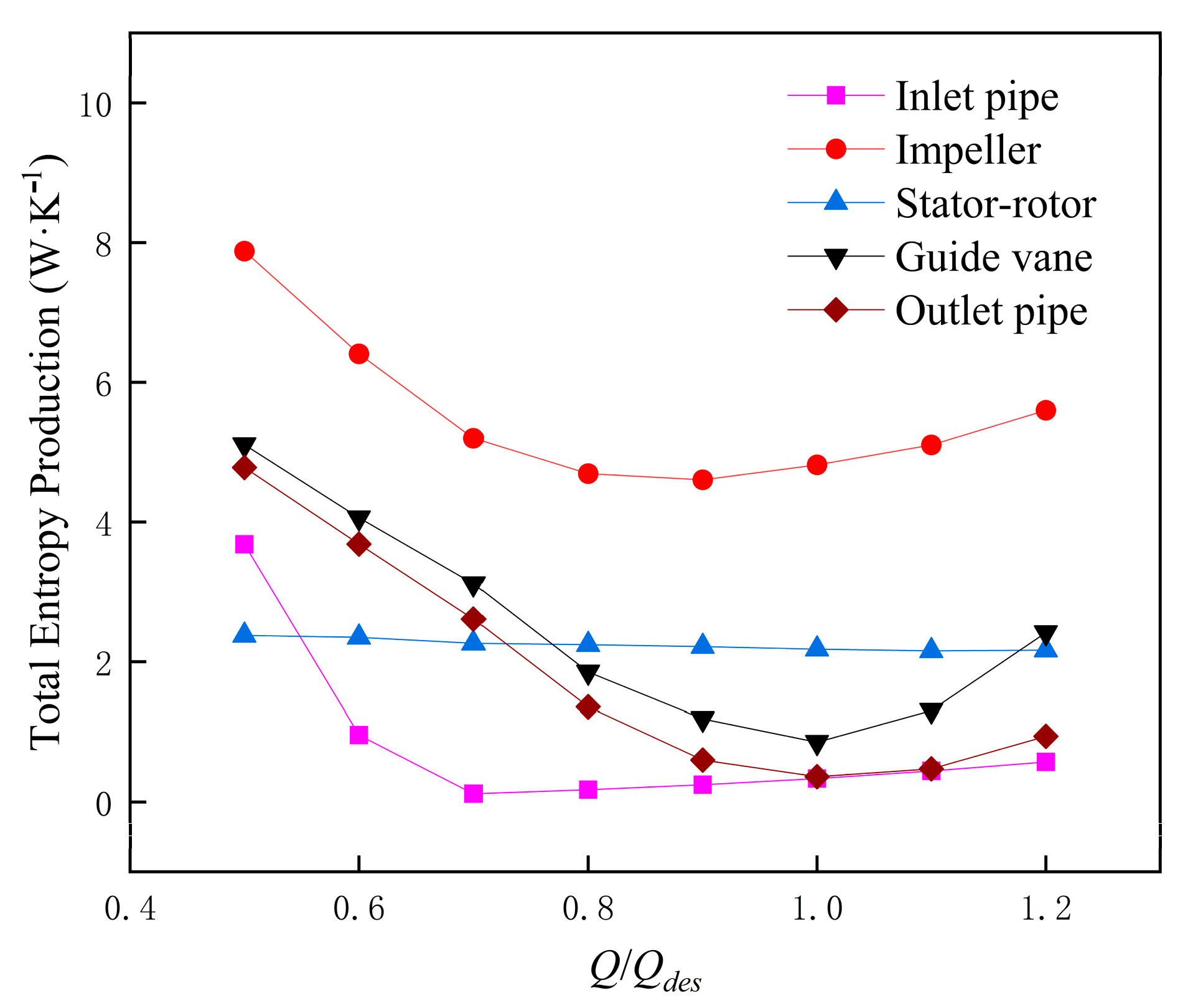
4.1. ΔS_pro of Each Flow Channel Component for FTP

Figure 6 shows the total entropy generation (ΔS_pro) of each flow channel component. Among all the components of the FTP, ΔS_pro in the impeller area was the highest, the minimum value exceeded 7 W·K⁻¹, and the ΔS_pro in the impeller area increased rapidly with the decrease in flow. The ΔS_pro in the stator–rotor area did not fluctuate significantly with the change in flow conditions, and the average value was about 2.2 W·K⁻¹. Under the design conditions, its ΔS_pro ratio was only second to the impeller, but with the decrease in flow, the ΔS_pro ratio at the stator–rotor gradually decreased to the lowest ratio among different flow channel components. The ΔS_pro in the guide vane area was smaller than 0.852 W·K⁻¹ at 1.0 Q_des, but with the change in flow rate, it is obvious that the ΔS_pro in this zone increased rapidly. The ΔS_pro of the outlet pipe was as small as that of the guide vane in the design condition, but it increased rapidly with the decrease in the flow rate, which indicates that the flow pattern of the guide vane and the outlet pipe of the FTP can be optimized in the future operation process. Near the high efficiency range, the ΔS_pro value of the inlet pipe was the smallest among all flow channel components. However, with the flow rate decreasing to 0.6 Q_des, the ΔS_pro of the inlet pipe had a sudden change, and the overall proportion was also increasing rapidly. This shows that under small flow conditions, the bad flow patterns such as the clearance backflow between the stator and rotor of the FTP and the vortex affect the inlet flow pattern, which makes the energy loss of the inlet pipe increase rapidly. From this figure, the dissipation of the FTP near the saddle zone is mainly reflected in the impeller, inlet pipe, and outlet pipe, which will be further analyzed in the following sections.

4.2. Comparison of Entropy Drop and Pressure Drop

The traditional calculation of hydraulic loss is called the pressure drop method, which can only quantitatively study the value of a certain area, and cannot be described in the figure. The entropy method for calculating hydraulic loss is simply called the entropy drop method, which has the advantage of visualizing dissipation distribution in the fluid domain [37]. In order to judge the applicability of the entropy generation theory in the FTP, this paper compares the hydraulic losses obtained by the two methods. Entropy loss (h_ep) is composed of ΔS_pro,TE, ΔS_pro,DE, and ΔS_pro,WE. The specific calculation formula is shown in (14). The entropy generation unit above the right side of the equation is W·K⁻¹, and the temperature unit is K. Among them, W is also kg·m²·s⁻³, and according to the unit system, the unit on the right side of the equation is also m. For the pressure drop loss (h_p) in the FTP, we calculated the hydraulic loss in the static parts such as the inlet pipe, guide vane, and outlet pipe according to the total pressure difference between inlet and outlet, with the specific formula shown in (15). The total pressure loss in the impeller and stator–rotor area of the rotating part was obtained by subtracting the work performed by the inlet and outlet pressure difference from the input power in this zone. The specific formula is shown in (16), where W_s is the input power and its unit is W.

$$h_{ep}=\frac{(\Delta S_{pro,TE}+\Delta S_{pro,DE}+\Delta S_{pro,WE})\cdot T}{\rho gQ}$$

(14)

$$h_p=\frac{p_{in}-p_{out}}{\rho g}$$

(15)

$$h_p=\frac{W_S}{\rho gQ}-\frac{p_{out}-p_{in}}{\rho g}$$

(16)

In order to compare the entropy drop loss and pressure drop loss more intuitively, K is used to represent the ratio of entropy drop loss and pressure drop loss under different flow conditions, as shown in (17).

$$K=\frac{h_{ep}}{h_p}$$

(17)

Figure 7 shows the comparison of the entropy drop loss and pressure drop loss of the FTP. It can be seen that the ratio of the inlet pipe tends to be stable and starts to decrease at 0.6 Q_des. The ratio of outlet pipe fluctuates at 0.8. The ratio K of the impeller fluctuates between 0.75 and 1.50. The ratio at 1.0 Q_des is larger than 1.5, but the difference between the two losses is small. The h_p is 0.244 m, and the h_ep is 0.376 m. The reason for the decrease in the ratio of small flow rate may be the high speed and strong flow in the impeller region. The ratio of the guide vane fluctuates between 0.75 and 1.08, and the smaller the flow rate, the closer the K value is to 1, indicating that the h_p and h_ep tend to be consistent under small flow conditions. The ratio at the stator–rotor fluctuates between 0.9 and 1.4, and is close to 1 under small flow conditions. On the whole, the trend of h_ep is consistent with h_p, which indicates that the entropy generation theory is applicable to the FTP. The entropy generation of different flow channel components is analyzed in detail below.

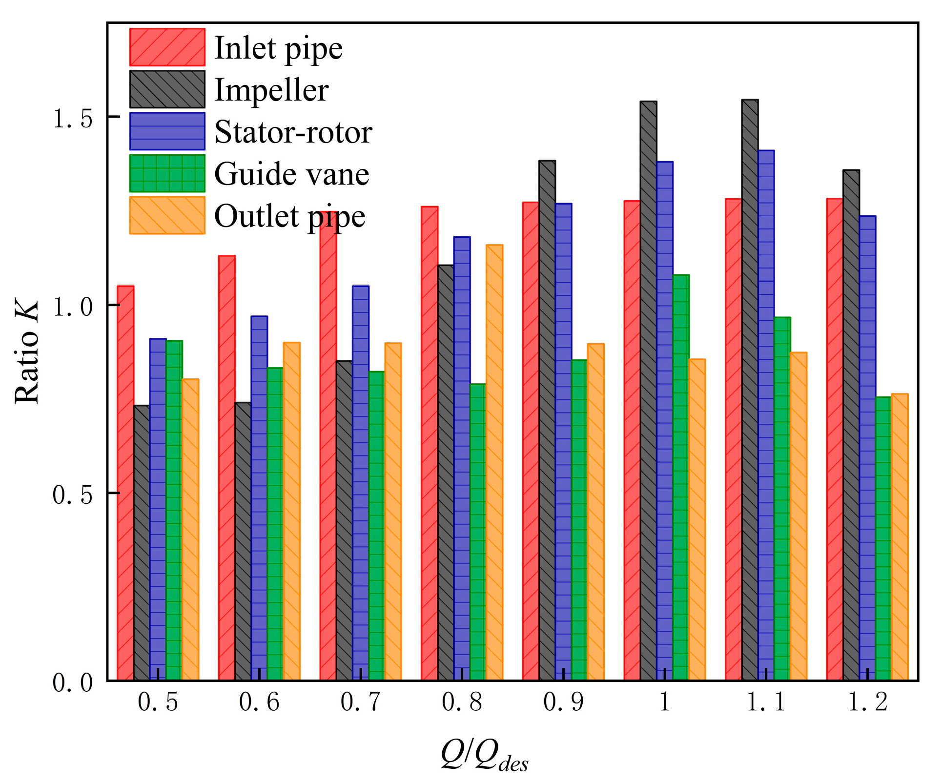
4.3. Proportion of Different FTP Components’ Entropy Production

Figure 8a shows the ΔS_pro,TE of different flow channel components. From the figure, it can be seen that the ΔS_pro,TE of the impeller under the design condition is much higher than that of the other flow channel components, and its value is the highest; especially under small flow conditions, the ΔS_pro,TE increases rapidly. ΔS_pro,TE in the stator–rotor region is very small, at about 0.4W·K⁻¹, and its values do not change with the operating conditions. The change in the guide vane and outlet pipe is the same, and the proportion of the ΔS_pro,TE in the channel is small, under 1.0 Q_des. However, as shown in Figure 5 above, the FTP enters the small flow condition at 0.8 Q_des, forming a serious saddle zone at 0.6 Q_des. The ΔS_pro,TE at the guide vane and outlet pipe increase sharply when entering the small flow condition.

Figure 8b shows the ΔS_pro,WE of different flow channel components. The ΔS_pro,WE in the impeller area decreases with the decrease in flow, and the value is 2.69 W·K⁻¹ under 1.0 Q_des. The change trend in ΔS_pro,WE at the stator–rotor is the same as that in ΔS_pro,TE, and the average value is 1.9 W·K⁻¹. The ΔS_pro,WE value of the guide vane area is small. Although it increases under small flow conditions, it does not exceed 1.3 W·K⁻¹ as a whole. Different from the ΔS_pro,TE of the inlet pipe, the ΔS_pro,WE of the outlet pipe does not change with changes in operating conditions.

Figure 8c shows the ΔS_pro,DE of different flow channel components. The ΔS_pro,DE of the flow channel components, except the impeller, are very small, all within 0.005 W·K⁻¹. The ΔS_pro,DE of the impeller decreases with the change in the operating conditions, which is 0.042 W·K⁻¹ under 1.0 Q_des. Since the ΔS_pro,DE accounts for less than 1% of the ΔS_pro, Figure 8d shows the proportion of ΔS_pro,TE and ΔS_pro,WE when the ΔS_pro,DE is ignored. The ΔS_pro,WE of the FTP is 28.2% higher than the ΔS_pro,TE under the design condition, but the proportion of ΔS_pro,TE increases rapidly under the small flow condition, and even exceeds 70% at the saddle zone. Therefore, the ΔS_pro,TE of the FTP will be mainly analyzed in the following analysis.

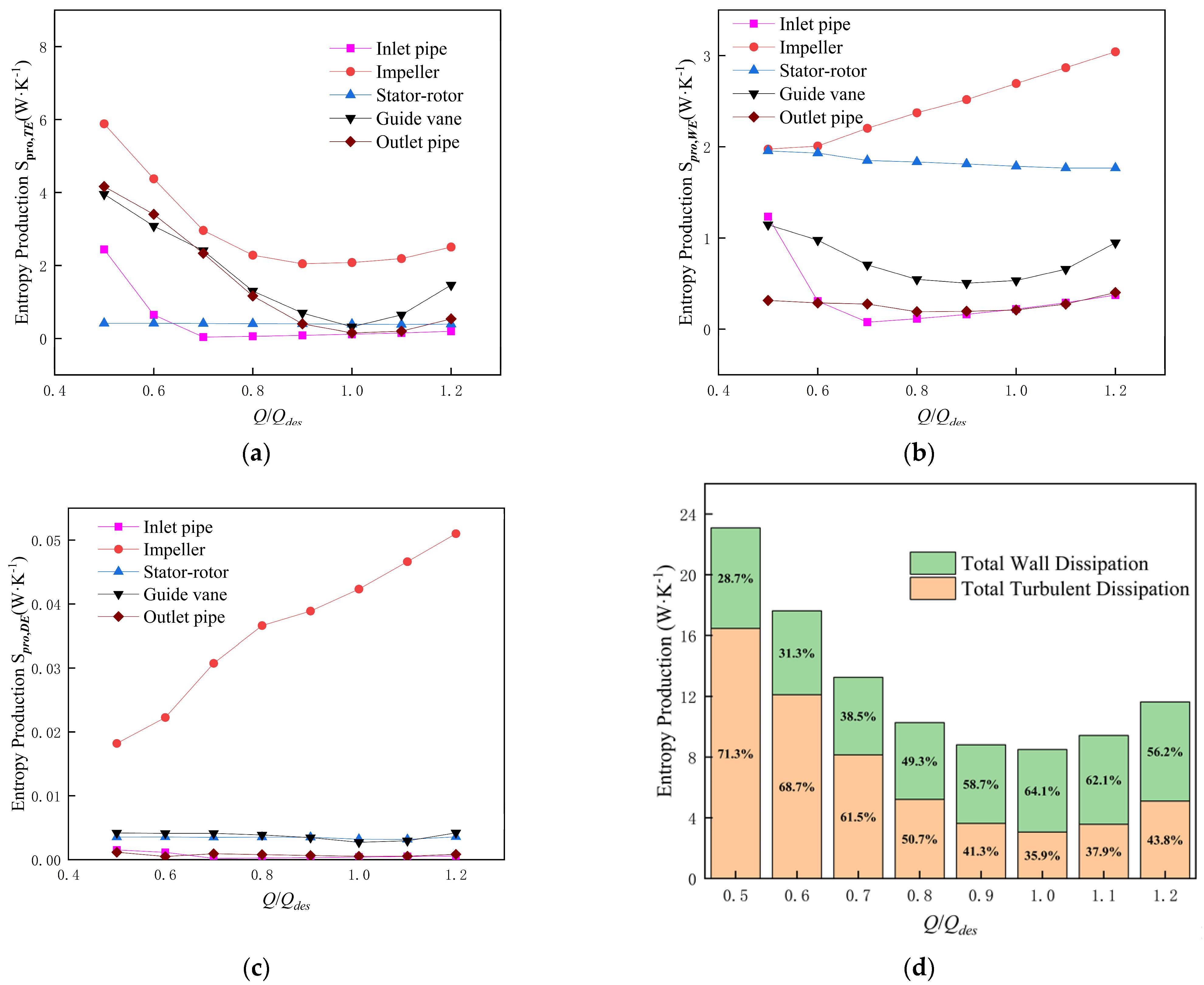
4.4. Distribution of S_TE under Typical Section of Each Flow Channel Component

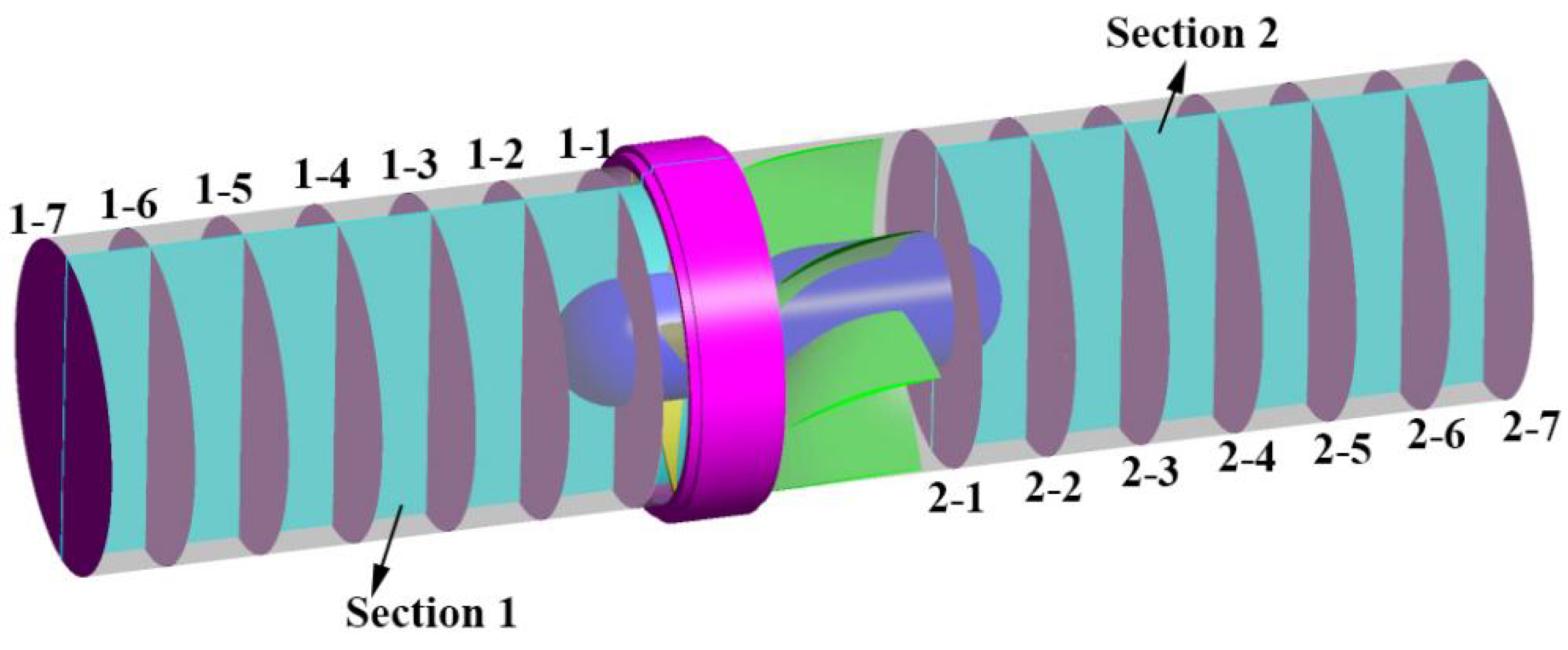
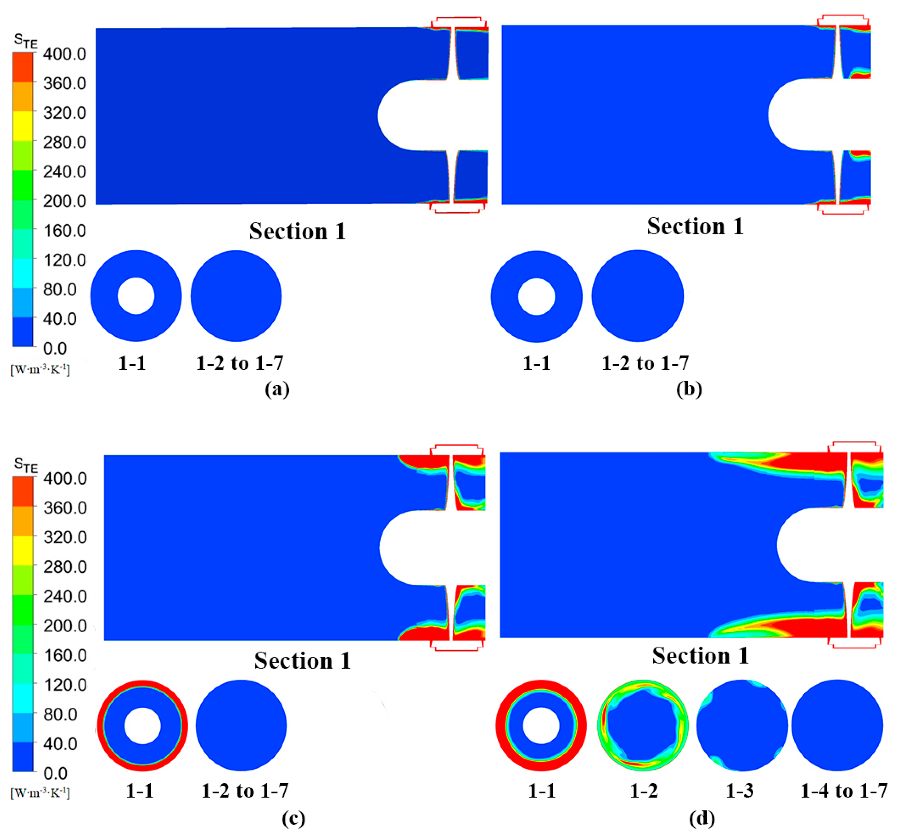
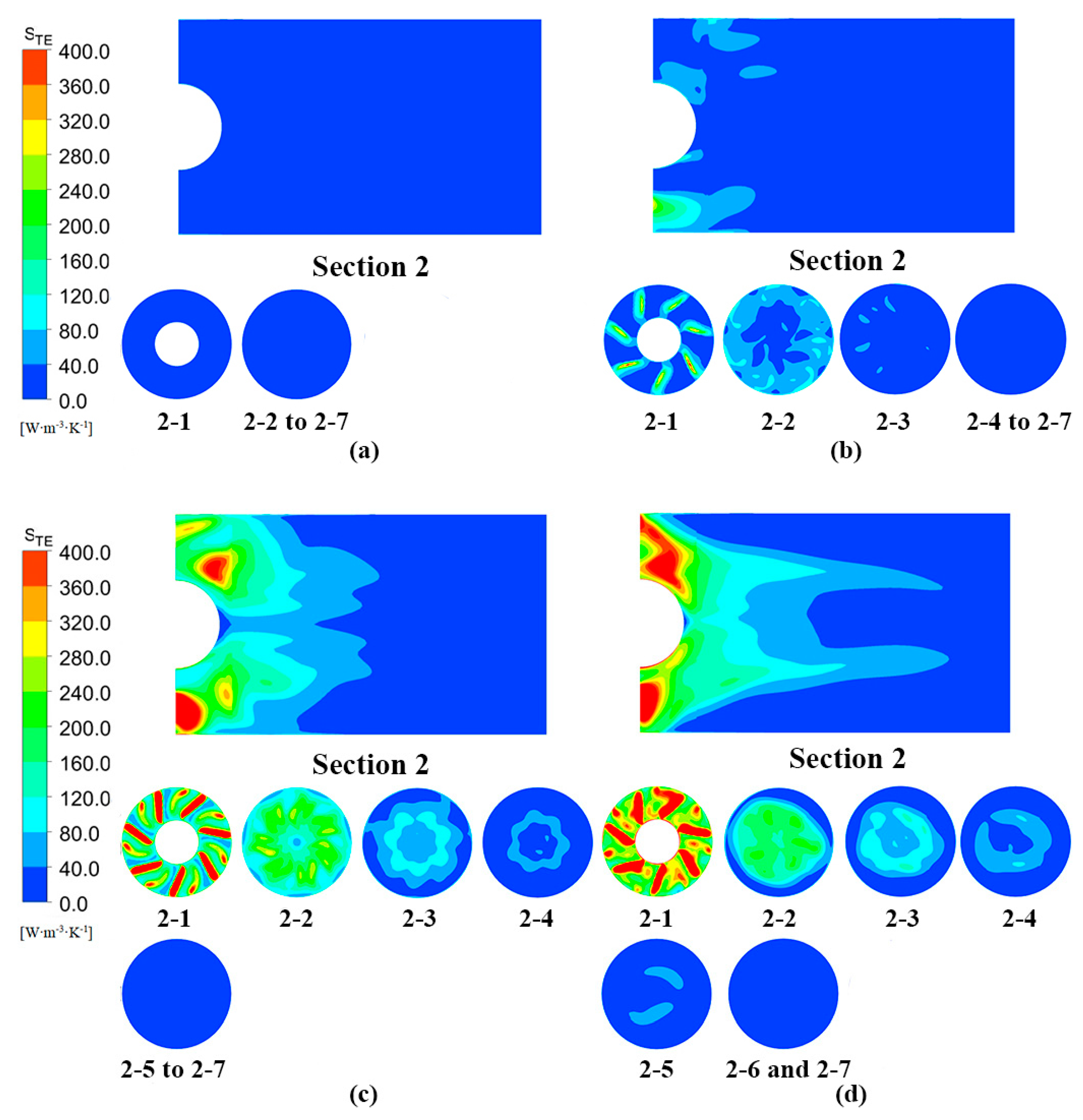
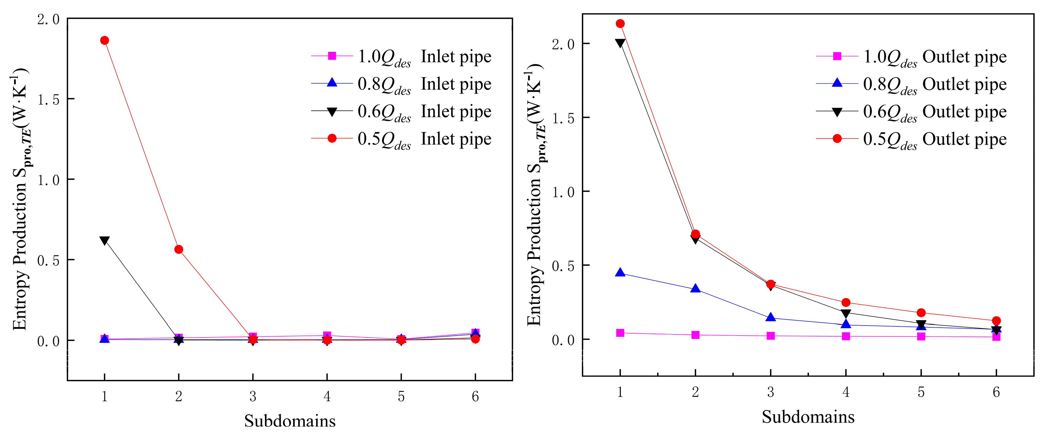
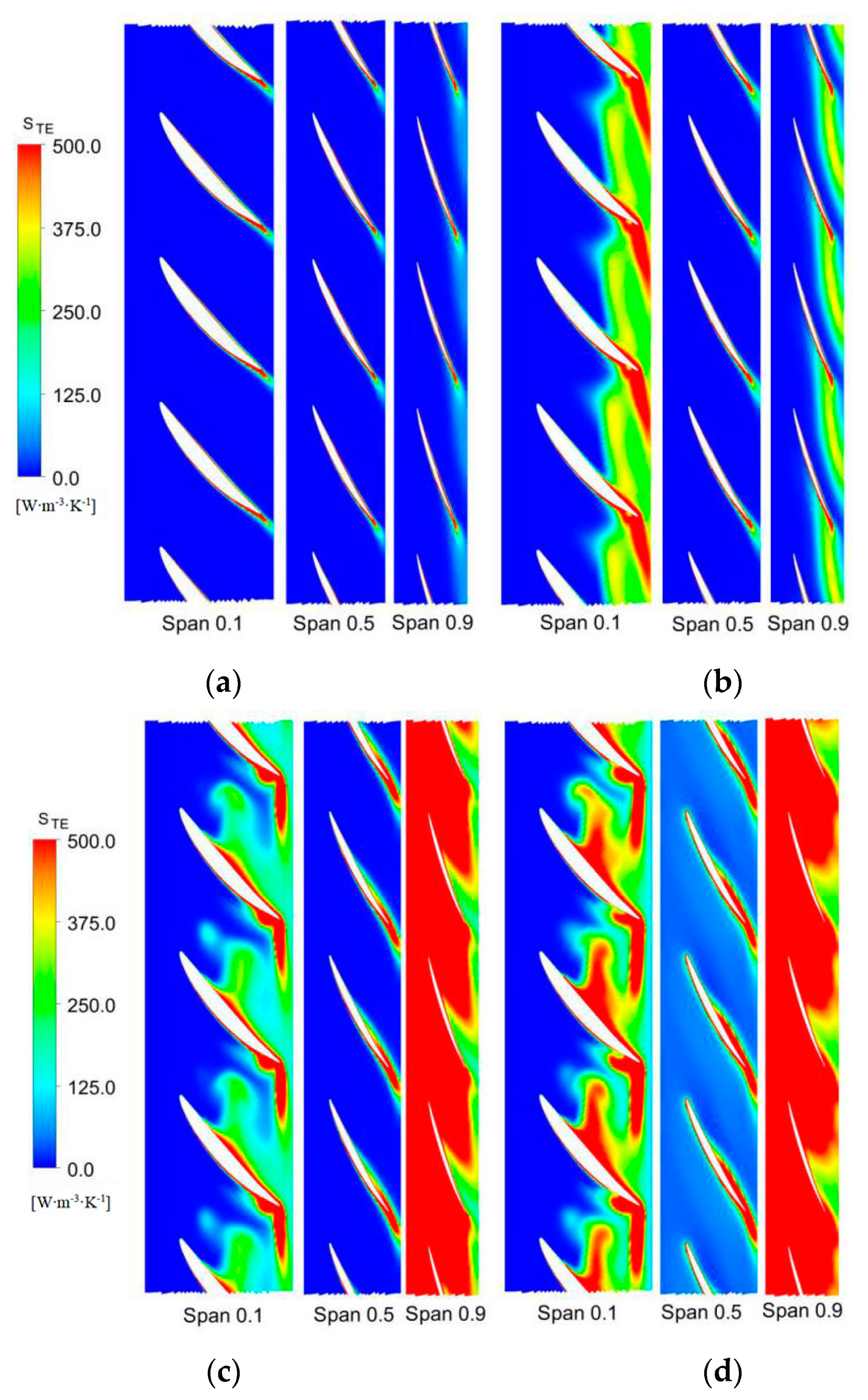
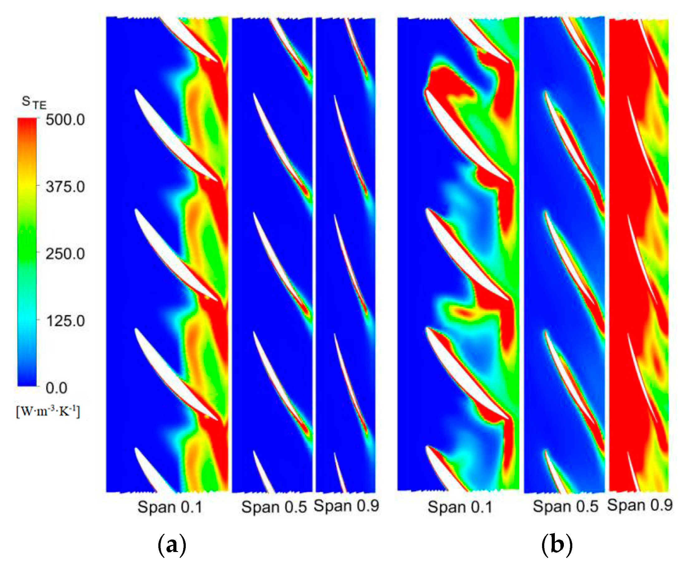
4.4.1. Distribution of S_TE under Typical Sections of Inlet and Outlet Pipe

Figure 9 is an analysis of the typical sections of the FTP, where Section 1 represents the central sections of the inlet pipe, impeller, and stator–rotor, and Sections 1-1 to 1-7 are equidistant from the inlet pipe outlet to the inlet. Section 2 represents the central section of the outlet pipe, and Sections 2-2 to 2-7 are equidistant from the outlet pipe inlet to the outlet. Figure 10 shows the high S_TE distribution of the typical section of the inlet pipe. At 1.0 Q_des, because the width of the backflow clearance is just 0.65 mm, only the stator–rotor has a high S_TE range. When the flow rate begins to decrease, firstly, the S_TE increases at the shroud of the blade due to the flow separation, and a small high S_TE range also appears at the inlet of the backflow clearance between the stator and rotor due to the 90° turning when the flow enters. When entering stall condition 0.6 Q_des, the clearance backflow causes the flow field near the impeller inlet to be disordered, and a high S_TE range appears rapidly. When entering the deep stall condition 0.5 Q_des, the clearance backflow not only affects the flow field at the impeller inlet; the vortex and backflow caused by the clearance backflow also severely squeeze the flow pattern of the inlet pipe, which makes the S_TE at the outlet side wall of the inlet pipe also begin to increase.

Figure 11 shows the distribution of a high S_TE on a typical section of the outlet pipe. At 1.0 Q_des, the outlet pipe has no high dissipation range. At 0.8 Q_des, seven high dissipation ranges corresponding to guide vane blades are found at the inlet section of the outlet pipe, and the high S_TE decreases rapidly with the distance, indicating that the role of the guide vane in the dissipation rectification is obvious. Under the conditions of 0.6 Q_des and 0.5 Q_des in the stall zone, the dissipation rectification of the guide vanes is limited due to the enhancement of turbulence of flow. There are not only seven high S_TE ranges at the inlet of the outlet pipe, but also high S_TE ranges in the channel between the guide vane blades. Section 2 in (c) and (d) shows that the high dissipation range almost diffuses to the entire outlet pipe.

In order to explain the ΔS_pro,TE value of the inlet and outlet pipes due to clearance backflow and vortex in detail, we divide the different sections of the inlet and outlet pipes in Figure 9 into different sub-volume domains (for example, 1-1 to 1-2 are sub-volume domains 1#, and 1-2 to 1-3 are sub-volume domains 2#, then continuing recursively. The same is true for the outlet pipe). As seen in Figure 12, the values of ΔS_pro,TE in the inlet pipe tend to be stable at the position where the distance is far from the impeller. At 0.5 Q_des, the dissipation value of the inlet pipe caused by clearance backflow is 3.0 times that in the sub-volume domain 1# at 0.6 Q_des, which indicates that although the ΔS_pro,TE at the stator–rotor does not increase with the decrease in flow, its clearance backflow seriously affects the ΔS_pro,TE value at the outlet section of the inlet pipe, and the smaller the flow, the more the ΔS_pro,TE value at the outlet section increases by a geometric number. Similarly, the ΔS_pro,TE of the outlet pipe is unevenly distributed under small flow conditions, and the high dissipation value is mainly reflected in the inlet section and accounts for about half of the total value. Under small flow conditions, the ΔS_pro,TE value from the inlet sub-volume domain 1# to the sub-volume domain 2# decreases by 60%.

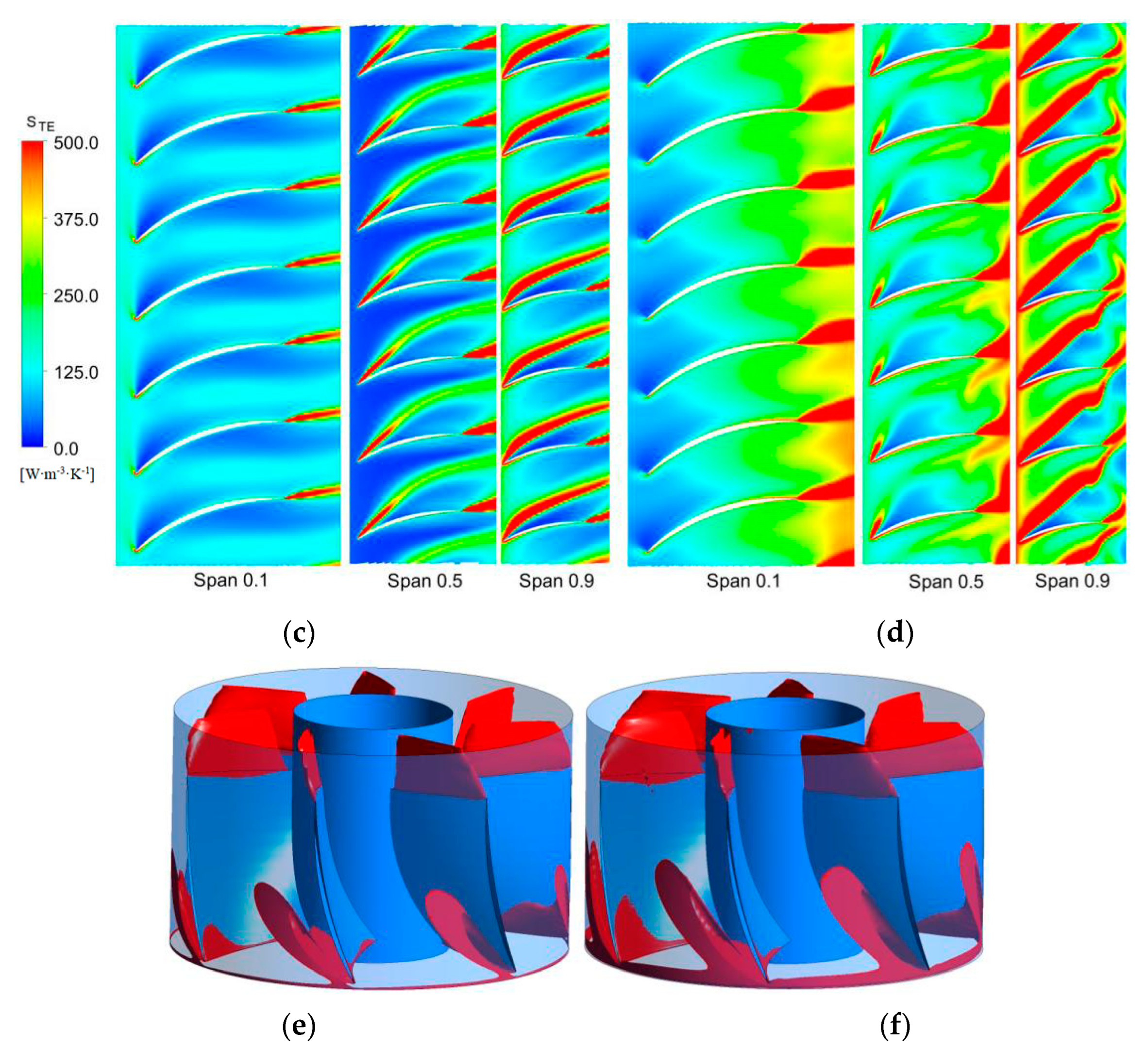
4.4.2. Distribution of S_TE under Typical Sections of the Impeller

According to Section 4.3, under stall condition, most of the energy is lost by S_TE, and the impeller is the main area of S_TE. We selected the contour surfaces of different impeller blade spans to analyze the S_TE in the impeller (Span = 0.1 means close to the hub, Span = 0.9 means close to the shroud, and a, b, c, and d, respectively, represent 1.0 Q_des, 0.8 Q_des, 0.6 Q_des, and 0.5 Q_des). Figure 13a shows that the S_TE of the whole blade is very small at 1.0 Q_des, and the high S_TE range mainly appears in the outlet area of the blade suction surface. Figure 13b shows that at 0.8 Q_des, the S_TE at the outlet of the blade suction surface at Span = 0.1 starts to increase and starts to diffuse to the blade pressure surface and the impeller channel. The reason for this phenomenon is that the flow separation at the trailing edge of the blade when the flow decreases makes the velocity of the blade channel inconsistent with the surface velocity of the blade, resulting in a vortex, leading to the turbulent dissipation beginning to spread out there. Similarly, at Span = 0.9, the flow separation on the suction surface of the blade also makes the high dissipation zone diffuse to the blade channel. The S_TE at Span = 0.5 is not much different from that at 1.0 Q_des, indicating that the blade flow field under this blade span is still good.

When entering stall zone (0.6 Q_des), it is evident that the S_TE extends to the leading edge at Span = 0.1; the high dissipation begins to affect the S_TE of the blade channel on the same side. However, at Span = 0.9, the flow backflows to the impeller inlet through the clearance of the stator–rotor, and the S_TE in the blade inlet and channel increases rapidly. The smaller the flow, the greater the clearance backflow. Therefore, the reason for the formation of the stall zone is that when the flow decreases to a certain extent, the flow field at the impeller inlet is affected by the backflow of the stator–rotor clearance, which leads to a rapid increase in the S_TE in the blade inlet and channel. When entering deep stall condition (0.5 Q_des), the S_TE at Span = 0.1 begins to spread further, and the high S_TE dissipation range is at the trailing edge of the suction surface and the middle edge of the pressure surface of the blade. At Span = 0.9, the S_TE continues to increase at the blade outlet.

The above analysis shows that when the flow decreases to below 1.0 Q_des, the S_TE in the impeller region is mainly reflected in the flow separation of the blade trailing edge at Span = 0.1 near the hub. When the flow is reduced to the stall zone, the S_TE at Span = 0.9 near the shroud increases rapidly due to the backflow of the stator–rotor clearance, which is much larger than the S_TE under other blade spans.

In order to further illustrate that it is the clearance backflow between the stator and rotor that affects the inlet flow field of the FTP, the condition in the stall zone of the FTP (0.6 Q_des, 0.5 Q_des) was selected to be compared with that of the AFP. After the stator and rotor are removed from Figure 14a, at 0.6 Q_des, the S_TE of the blade trailing edge near the hub at Span = 0.1 is higher than that of the FTP, but the flow field at Span = 0.9 is much better than that of the FTP, and only a small range of high S_TE exists at the trailing edge of the blade suction surface. When entering deep stall condition (0.5 Q_des), the inlet flow field at Span = 0.9 near the shroud starts to be disordered, and the S_TE value starts to increase sharply. Comparing Figure 13c with Figure 14a, due to the clearance between the stator and rotor, when the flow condition is reduced to a certain extent, the inlet flow field of the FTP near the shroud is disordered in advance, resulting in the surge in S_TE there, and the stall zone is advanced.

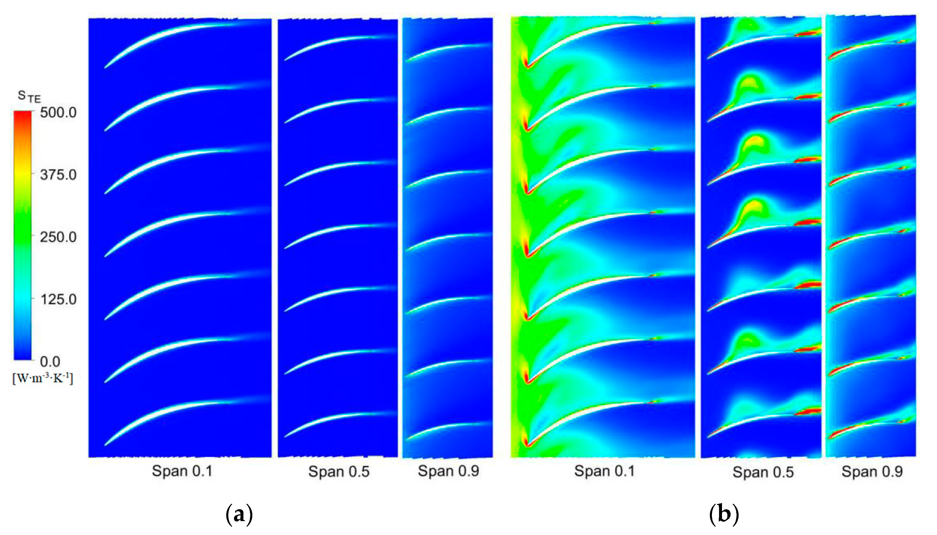
4.4.3. Distribution of S_TE under Typical Sections of Guide Vane

Further analyzing the S_TE at the guide vane, Figure 15 shows the S_TE of the guide vane with different spans, in which Figure 15e,f show the S_TE isosurface of ΔS_pro,TE = 1 × 10³ W·m⁻³·K⁻¹ in the channel. The S_TE of the guide vane with different spans is much smaller than that of the impeller, and there is no high S_TE range in the guide vane at 1.0 Q_des. When the operating condition changes, the high S_TE range appears at the leading edge of the inlet, and also at the trailing edge of the suction surface of the guide vane due to the flow separation. In the stall condition, the high S_TE range of the leading edge of the blade diffuses to the blade channel, and the high S_TE range of the trailing edge diffuses to the blade outlet. From the S_TE isosurface in Figure 15e,f, we found that under the stall condition, the high dissipation range at the guide vane of the FTP mainly exists at the channel near the suction surface and at the downstream of the outlet along the tangent direction.

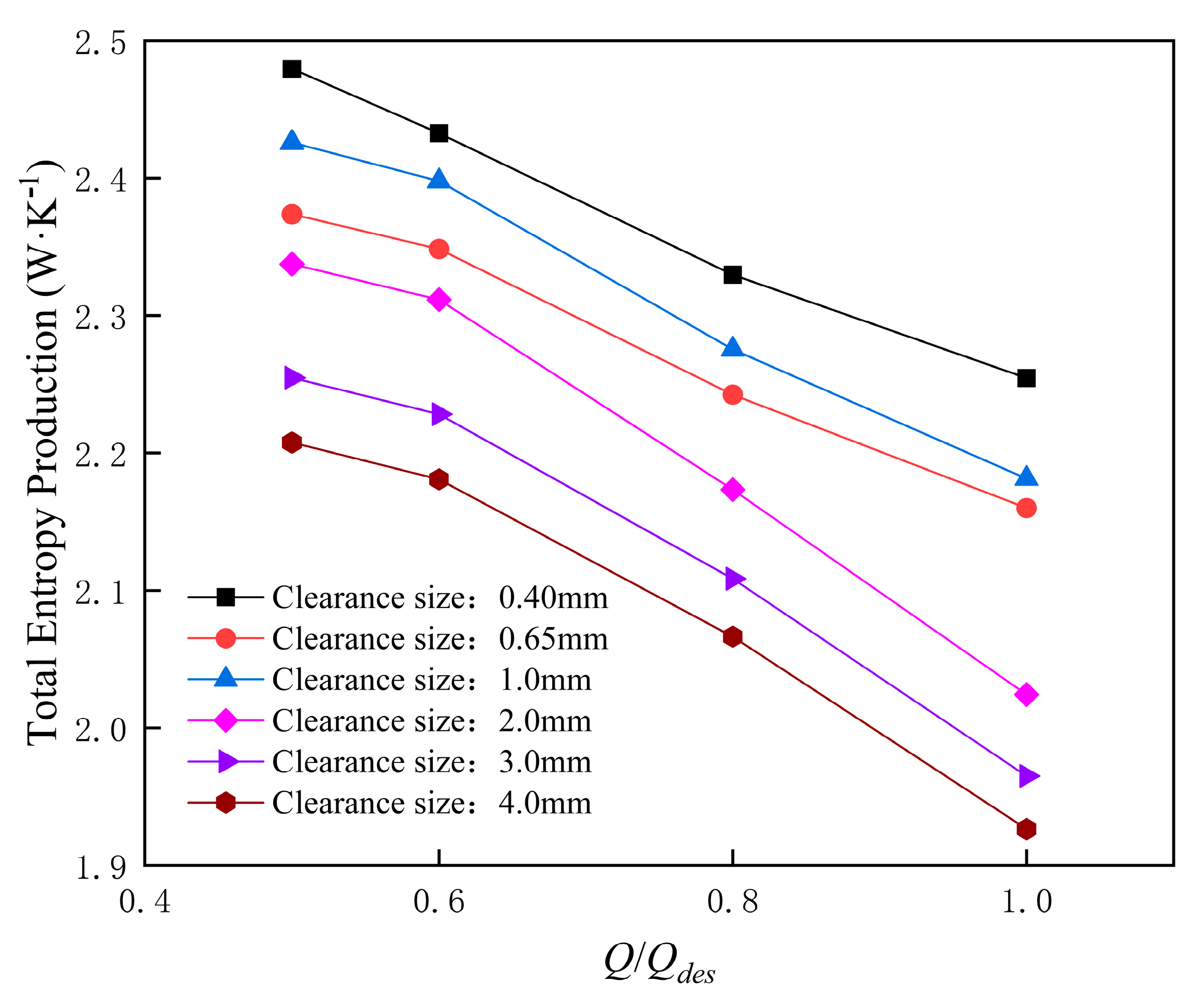
4.5. Influence of Backflow Clearance Size to ΔS_pro

Because the ΔS_pro at the stator–rotor is not sensitive to the change in flow, in order to specifically analyze that the ΔS_pro at the backflow clearance between the stator and rotor is mainly affected by a certain parameter, the ΔS_pro value of the stator–rotor is compared by selecting different backflow clearance sizes. The specific sizes include 0.4 mm, 0.65 mm (the size used in the numerical simulation and experiment in this paper), 1.0 mm, 2.0 mm, 3.0 mm, and 4.0 mm. Figure 16 shows the ΔS_pro in the stator–rotor with different backflow clearance sizes. When the flow rate decreases, the ΔS_pro in different clearance sizes increases, but the increased amplitude is much smaller than that of other flow channel components. The larger the backflow clearance size, the more the ΔS_pro value at the stator–rotor decreases. The change in the ΔS_pro value caused by the change in the backflow clearance size of the stator–rotor is more obvious than that caused by the flow condition, which indicates that the backflow clearance size at the stator–rotor is the main reason that affects the ΔS_pro value of the stator–rotor.

5. Conclusions

Compared with the conventional AFP, the FTP has a more serious saddle zone under small flow conditions. After the comparison of the numerical simulation and physical tests to verify the accuracy of the external characteristics, we used the entropy generation theory to study the cause and distribution of the energy loss of the FTP under the stall conditions of the FTP. The conclusions are as follows:

(1)

Under stall conditions, the FTP is affected by 90° clearance backflow, resulting in a rapid increase in S_TE within the wall range of the sub-volume domain at the outlet of the inlet pipe. At the same time, the outlet pipe is affected by the guide vanes, resulting in seven high dissipation ranges in the inlet section. The high S_TE region of the guide vane appears where there is flow separation, that is, the leading edge of the guide vane inlet and the trailing edge of the blade.

(2)

The high S_TE in the impeller first occurs in the outlet flow separation region of the suction surface of the blade. At the stall condition, the influence of the clearance backflow between the stator and rotor makes the inlet flow field of impeller disordered in advance. The high S_TE quickly fills the whole impeller, which affects the working ability of the impeller, and makes the stall zone of the FTP advance macroscopically.

(3)

Compared with the changes caused by the flow conditions, the backflow clearance size at the stator–rotor of the FTP is the main reason for the dissipation of the stator–rotor. The larger backflow clearance causes a smaller dissipation at the stator–rotor. In engineering practice, the size of reflow clearance should be reasonably arranged in consideration of the actual requirements.

References

1. Liu, C. Researches and developments of axial-flow pump system. Trans. Chin. Soc. Agric. Mach. 2015, 46, 49–59. [Google Scholar]
2. Gu, Z. Development and application of a new type submersible tubular pump. Water Resour. Hydropower Eng. 2010, 41, 54–57. [Google Scholar]
3. Shi, L.; Jiao, H.; Gou, J.; Yuan, Y.; Tang, F.; Yang, F. Influence of backflow gap size on hydraulic performance of full-flow pump. Trans. Chin. Soc. Agric. Mach. 2020, 51, 139–146. [Google Scholar]
4. Shi, L.; Zhang, W.; Jiao, H.; Tang, F.; Wang, L.; Sun, D.; Shi, W. Numerical simulation and experimental study on the comparison of the hydraulic characteristics of an axial-flow pump and a full tubular pump. Renew. Energy 2022, 153, 1455–1464. [Google Scholar] [CrossRef]
5. Shi, L.; Jiang, Y.; Cai, Y.; Chen, B.; Tang, F.; Xu, T.; Zhu, J.; Chai, Y. Influence of Inlet Groove on Flow Characteristics in Stall Condition of Full-Tubular Pump. Front. Energy Res. 2022, 10, 949639. [Google Scholar] [CrossRef]
6. Zhou, L.; Hang, J.; Bai, L.; Krzemianowski, Z.; Emam, E.; Yasser, E.; Agarwal, R. Application of entropy production theory for energy losses and other investigation in pumps and turbines: A review. Appl. Energy 2022, 318, 119211. [Google Scholar] [CrossRef]
7. Ji, L.; Li, W.; Shi, W.; Tian, F.; Agarwal, R. Effect of blade thickness on rotating stall of mixed-flow pump using entropy generation analysis. Energy 2021, 236, 121381. [Google Scholar] [CrossRef]
8. Gu, Y.; Pei, J.; Yuan, S.; Wang, W.; Zhang, F.; Wang, P.; Appiah, D.; Liu, Y. Clocking Effect of Vaned Diffuser on Hydraulic Performance of High-Power Pump by Using the Numerical Flow Loss Visualization Method. Energy 2019, 170, 986–997. [Google Scholar] [CrossRef]
9. Shen, S.; Qian, Z.; Ji, B. Numerical Analysis of Mechanical Energy Dissipation for an Axial-Flow Pump Based on Entropy Generation Theory. Energies 2019, 12, 4162. [Google Scholar] [CrossRef]
10. Shen, S.; Huang, B.; Huang, S.; Xu, S.; Liu, S. Research on Cavitation Flow Dynamics and Entropy Generation Analysis in an Axial Flow Pump. J. Sens. 2022, 18, 7087679. [Google Scholar] [CrossRef]
11. Zhang, X.; Tang, F. Energy loss evaluation of axial flow pump systems in reverse power generation operations based on entropy production theory. Sci. Rep. 2022, 12, 8667. [Google Scholar] [CrossRef]
12. Yang, F.; Li, Z.; Cai, Y.; Jiang, D.; Tang, F.; Sun, S. Numerical Study for Flow Loss Characteristic of an Axial-Flow Pump as Turbine via Entropy Production Analysis. Processes 2022, 10, 1695. [Google Scholar] [CrossRef]
13. Yang, F.; Li, Z.; Hu, W.; Liu, C.; Jiang, D.; Liu, D.; Nasr, A. Analysis of flow loss characteristics of slanted axial-flow pump device based on entropy production theory. R. Soc. Open Sci. 2022, 9, 211208. [Google Scholar] [CrossRef]
14. Pei, J.; Meng, F.; Li, Y.; Yuan, S.; Chen, J. Effects of distance between impeller and guide vane on losses in a low head pump by entropy production analysis. Adv. Mech. Eng. 2016, 8, 1–11. [Google Scholar] [CrossRef]
15. Kan, K.; Xu, Z.; Chen, H.; Xu, H.; Zheng, Y.; Zhou, D.; Muhirwa, A.; Maxime, B. Energy loss mechanisms of transition from pump mode to turbine mode of an axial-flow pump under bidirectional conditions. Energy 2022, 257, 124630. [Google Scholar] [CrossRef]
16. Kan, K.; Zhang, Q.; Xu, Z.; Zheng, Y.; Gao, Q.; Shen, L. Energy loss mechanism due to tip leakage flow of axial flow pump as turbine under various operating conditions. Energy 2022, 255, 124532. [Google Scholar] [CrossRef]
17. Yu, A.; Li, L.; Ji, J.; Tang, Q. Numerical study on the energy evaluation characteristics in a pump turbine based on the thermodynamic entropy theory. Renew. Energy 2022, 195, 766–779. [Google Scholar] [CrossRef]
18. Meng, F.; Li, Y. Energy Characteristics of a Bidirectional Axial-Flow Pump with Two Impeller Airfoils Based on Entropy Production Analysis. Entropy 2022, 24, 962. [Google Scholar] [CrossRef]
19. Li, Y.; Zheng, Y.; Meng, F.; Osman, K. The Effect of Root Clearance on Mechanical Energy Dissipation for Axial Flow Pump Device Based on Entropy Production. Processes 2020, 8, 1506. [Google Scholar] [CrossRef]
20. Li, D.; Gong, R.; Wang, H.; Xiang, G.; Wei, X.; Qin, D. Entropy production analysis for hump characteristics of a pump turbine model. Chin. J. Mech. Eng. 2016, 29, 803–812. [Google Scholar] [CrossRef]
21. Chang, H.; Shi, W.; Li, W.; Liu, J. Energy Loss Analysis of Novel Self-Priming Pump Based on the Entropy Production Theory. J. Therm. Sci. 2019, 28, 306–318. [Google Scholar] [CrossRef]
22. Kan, K.; Zheng, Y.; Chen, Y.; Xie, Z.; Yang, G.; Yang, C. Numerical study on the internal flow characteristics of an axial-flow pump under stall conditions. J. Mech. Sci. Technol. 2018, 32, 4683–4695. [Google Scholar] [CrossRef]
23. Li, W.; Ji, L.; Li, E.; Shi, W.; Agarwal, R.; Zhou, L. Numerical investigation of energy loss mechanism of mixed-flow pump under stall condition. Renew. Energy 2021, 167, 740–760. [Google Scholar] [CrossRef]
24. Ji, L.; Li, W.; Shi, W. Influence of tip leakage flow and inlet distortion flow on a mixed-flow pump with different tip clearances within the stall condition. Proc. Inst. Mech. Eng. Part A J. Power Energy 2020, 234, 433–453. [Google Scholar] [CrossRef]
25. Ceyrowsky, T.; Hildebrandt, A.; Schwarze, R. Numerical Investigation of the Circumferential Pressure Distortion Induced by a Centrifugal Compressor’s External Volute. In Proceedings of the ASME Turbo Expo 2018: Turbomachinery Technical Conference and Exposition, Oslo, Norway, 11–15 June 2018. [Google Scholar]
26. Cravero, C.; Marsano, D. Criteria for the Stability Limit Prediction of High Speed Centrifugal Compressors with Vaneless Diffuser: Part I—Flow Structure Analysis. In Proceedings of the Turbo Expo: Power for Land, Virtual, 21–25 September 2020; Sea, and Air. American Society of Mechanical Engineers: Houston, TX, USA. [Google Scholar] [CrossRef]
27. Cravero, C.; Marsano, D. Criteria for the Stability Limit Prediction of High Speed Centrifugal Compressors with Vaneless Diffuser: Part II—The Development of Prediction Criteria. In Proceedings of the Turbo Expo: Power for Land, Virtual, 21–25 September 2020; Sea, and Air. American Society of Mechanical Engineers: Houston, TX, USA. [Google Scholar] [CrossRef]
28. Mathieu, J.; Scott, J. An Introduction to Turbulent Flow; Cambridge University Press: Cambridge, MA, USA, 2000. [Google Scholar]
29. Kock, F.; Herwig, H. Entropy production calculation for turbulent shear flows and their implementation in CFD codes. Int. J. Heat Fluid Flow 2005, 26, 672–680. [Google Scholar] [CrossRef]
30. Kock, F.; Herwig, H. Local entropy production in turbulence shear flows: A high-Reynolds number model with wall functions. Int. J. Heat Mass Transf. 2004, 47, 2205–2215. [Google Scholar] [CrossRef]
31. Herwig, H.; Kock, F. Direct and indirect methods of calculating entropy generation rates in turbulent convective heat transfer problems. Heat Mass Transf. 2007, 43, 207–215. [Google Scholar] [CrossRef]
32. Bohle, M.; Fleder, A.; Mohr, M. Study of the losses in fluid machinery with the help of entropy. In Proceedings of the 16th International Symposium on Transport Phenomena and Dynamics of Rotating Machinery, Honolulu, HI, USA, 10–15 April 2016. [Google Scholar]
33. Xia, L.; Zou, Z.; Wang, Z.; Zou, L.; Gao, H. Surrogate model based uncertainty quantification of CFD simulations of the viscous flow around a ship advancing in shallow water. Ocean Eng. 2021, 234, 109206. [Google Scholar] [CrossRef]
34. Cravero, C.; De Domenico, D.; Marsano, D. The use of uncertainty quantification and numerical optimization to support the design and operation management of air-staging gas recirculation strategies in glass furnaces. Fluids 2023, 8, 76. [Google Scholar] [CrossRef]
35. Zhang, X.; Tang, F. Investigation of the hydrodynamic characteristics of an axial flow pump system under special utilization conditions. Sci. Rep. 2022, 12, 5159. [Google Scholar] [CrossRef]
36. Xu, T.; Cai, Y.; Chu, S.; Shi, L.; Zhu, J.; Jiang, Y. Hydraulic performance analysis of rear impeller of counter-rotating axial flow pump. J. Drain. Irrig. Mach. (JDIME) 2023, 41, 118–123, 138. [Google Scholar]
37. Yu, A.; Tang, Q.; Chen, H.; Zhou, D. Investigations of the thermodynamic entropy evaluation in a hydraulic turbine under various operating conditions. Renew. Energy 2021, 180, 1026–1043. [Google Scholar] [CrossRef]
Figure 1. 3D Calculation Model and Clearance Flow Schematic Diagram of FTP. (a) Full tubular pump, (b) Clearance flow of FTP, (c) Main design parameters of FTP.
Jmse 11 00895 g001
Figure 2. Computational fluid domain meshing.
Jmse 11 00895 g002
Figure 3. Grid-independent analysis of FTP.
Jmse 11 00895 g003
Figure 4. Field model test of FTP and AFP.
Jmse 11 00895 g004
Figure 5. Comparison of numerical simulation and model test.
Jmse 11 00895 g005
Figure 6. Distribution of ΔSpro of different flow channel components of FTP.
Jmse 11 00895 g006
Figure 7. Ratio K of entropy drop and pressure drop.
Jmse 11 00895 g007
Figure 8. Entropy generation distribution and proportion of different flow channels in the FTP. (a) ΔSpro,TE of different flow channel components, (b) ΔSpro,WE of different flow channel components, (c) ΔSpro,DE of different flow channel components, (d) the ratio of ΔSpro,TE to ΔSpro,WE.
Jmse 11 00895 g008
Figure 9. Typical cross-section of the FTP.
Jmse 11 00895 g009
Figure 10. Distribution of STE for a typical section of inlet pipe ((a) Q = 1.0 Qdes; (b) Q = 0.8 Qdes; (c) Q = 0.6 Qdes; (d) Q = 0.5 Qdes).
Jmse 11 00895 g010
Figure 11. Distribution of STE for typical section of outlet pipe ((a) Q = 1.0 Qdes; (b) Q = 0.8 Qdes; (c) Q = 0.6 Qdes; (d) Q = 0.5 Qdes).
Jmse 11 00895 g011
Figure 12. ΔSpro,TE values of different volume subdomains of inlet and outlet pipes.
Jmse 11 00895 g012
Figure 13. Distribution of STE for impeller with different spans ((a) Q = 1.0 Qdes; (b) Q = 0.8 Qdes; (c) Q = 0.6 Qdes; (d) Q = 0.5 Qdes).
Jmse 11 00895 g013
Figure 14. Distribution of STE for impeller with different spans in stall conditions when the stator and rotor are removed ((a) Q = 0.6 Qdes, (b) Q = 0.5 Qdes).
Jmse 11 00895 g014
Figure 15. Distribution of STE for guide vane with different spans and high STE isosurface distribution in the guide vane. ((a) Q = 1.0 Qdes; (b) Q = 0.8 Qdes; (c) Q = 0.6 Qdes; (d) Q = 0.5 Qdes; (e) high STE isosurface distribution when Q = 0.6 Qdes; (f) high STE isosurface distribution when Q = 0.5 Qdes)).
Jmse 11 00895 g015aJmse 11 00895 g015b
Figure 16. ΔSpro of stator–rotor region under different backflow clearance sizes.
Jmse 11 00895 g016