Machine Learning and Case-Based Reasoning for Real-Time Onboard Prediction of the Survivability of Ships

Abstract

The subject of damaged stability has greatly profited from the development of new tools and techniques in recent history. Specifically, the increased computational power and the probabilistic approach have transformed the subject, increasing accuracy and fidelity, hence allowing for a universal application and the inclusion of the most probable scenarios. Currently, all ships are evaluated for their stability and are expected to survive the dangers they will most likely face. However, further advancements in simulations have made it possible to further increase the fidelity and accuracy of simulated casualties. Multiple time domain and, to a lesser extent, Computational Fluid dynamics (CFD) solutions have been suggested as the next “evolutionary” step for damage stability. However, while those techniques are demonstrably more accurate, the computational power to utilize them for the task of probabilistic evaluation is not there yet. In this paper, the authors present a novel approach that aims to serve as a stopgap measure for introducing the time domain simulations in the existing framework. Specifically, the methodology presented serves the purpose of a fast decision support tool which is able to provide information regarding the ongoing casualty utilizing prior knowledge gained from simulations. This work was needed and developed for the purposes of the EU-funded project SafePASS.

1. Introduction

The maritime industry plays a crucial role in the global economy, with ships transporting a large proportion of goods and raw materials across the world. The safety of ships and their crew is of paramount importance, and damage stability is one of the key factors that determine the survival of a ship in the event of an accident. In this paper, we present a novel approach for the real-time prediction of damage stability outcomes using Case-based Reasoning (CBR) and Machine Learning (ML) models. CBR is a problem-solving approach that uses prior experience to solve new problems [1,2], while ML models are used to make predictions based on data after being trained on a relevant dataset. Our approach combines these two techniques to provide an accurate and efficient method for predicting damage stability outcomes in real-time, enabling crews to take appropriate action in the event of an emergency.

There are several existing real-time decision support tools for damage stability analysis in the maritime industry, including traditional methods such as rule-based systems and simulation models. Examples of traditional methods include relevant prepared paperwork such as damage stability plans, quick reference floodable length charts (used to judge survivability based on compartments damaged) or other rule-based standing orders and procedures. Since these items have physical properties and/or are focused on specific cases, they are not easily adjusted to evolving situations, especially if they deviate from the expected. An example of this can be found in the recent sinking of the Helge Ingstad, where non-continuous damages were evaluated by a carpet plot derived with the assumption of continuous damage [3]. Non-continuous damages and generally incomplete or erroneous understanding of the situation have contributed to various accidents [4].

A decision support tool that can assist during the emergency needs to assess the risk accurately and quickly. The proposed approach can forecast how the flooding will propagate and how the vessel will be affected in future instances while satisfying those two objectives. The most crucial functional requirements for the application of the proposed methods are:

(i)

the ability of the approach to receive and process ‘live data’ of the critical influencing parameters for the assessment of the risk, and

(ii)

to have a framework/tool/algorithm in place which can produce predictions and make projections within a short enough period of time so that it can be meaningful for on the spot crisis management support.

The accuracy is inherently linked with the capacity of the approach to make correct predictions; however, the challenge becomes significantly more demanding when you have to factor in the processing time of the analysis.

Flexible, computerized tools have been developed that normally use onboard sensor data to provide decision support [5,6,7]. While there are differences in each application, all methods share several processes. Namely, multiple sensor data are needed that are then used to estimate the breach size and location, populate and then solve a hydraulic model to predict the flooding extent and provide corrections to previous time-step solutions in a feedback loop. The individual parts of such a process have been studied extensively; including flooding models [8,9,10,11,12,13,14,15,16,17], the effect of non-watertight doors [18], sensors [19,20,21] and decision support systems [5,6,22,23]. Experimental investigations have also attempted to capture the underlying phenomena and validate tools for predicting the dynamics of the vessel-floodwater-seaway interaction [17,24,25,26,27]. In short, an ideal decision support system is able to use sensor data accurately to initialize a flooding simulation which is then run in the presence of external forces, and whose results can then be interpreted in a decision support framework and display useful data to the decision maker. The elusive part of this process has always been the accurate and timely capture of the physical phenomena involved. On one hand, fluid dynamics are exceedingly complicated at that scale and, similarly, the marine environment, especially in significant waves, is a chaotic and aleatoric amalgam of fluid-air interactions in various regimes.

Along the same lines, the EU-funded project SafePASS [28,29] strives to revolutionize the process of evacuation on large passenger ships. While the project’s many partners developed various technological solutions such as dynamic routing, augmented reality [30], smart lifejackets and wristbands [31], programmable exit signs and others [32], a critical piece of information is needed. Knowledge of the risk level of the current situation and, more importantly, the future end state, is crucial in determining whether to initiate an evacuation or not [33]. The flooding risk is of course dependent on the details of the loading of the vessel and its stability, as well as the extent of the damage to it. While many physical phenomena are captured by different methods, a tool that can evaluate the risk swiftly and robustly has to rely on a database of cases.

The methodology presented below was created to satisfy this need in real-time, with simplicity for the end user. Two distinct but ultimately similar methods are presented below: Case-Based Reasoning and Machine Learning, that independently can provide predictions based on “analyzing” the database. In this way, the lengthy and costly computations that describe the actual phenomena can be bypassed. At first, it would appear that this approach is simplistic or naïve, as it appears to disregard the physical events. While first principles methods rely on mathematical equations and physical laws to predict outcomes, machine learning can automatically learn patterns and relationships from data to make predictions or decisions. Additionally, machine learning can adapt and improve its predictions over time. Furthermore, increasing the data supplied to the model will also improve its capabilities. Case-based reasoning is also similarly able to utilize a database to create robust observations.

The methods are presented below with regard to their fundamentals as well as to the formulation adopted for the task at hand. A demonstrative implementation in simulated real-life scenario(s) is also added to showcase the performance and practical application of the methodology. The results suggest that this methodology warrants further study and experimentation.

2. Materials and Methods

2.1. Architecture

The architecture of the methodology largely follows two paths that have common starting and ending points. To be precise, both methods of obtaining predictions on the risk from flooding incidents originate from the same database and, after their respective processes, arrive at the same variable predictions. Their results can be isolated or examined in a combined manner. The following figure (Figure 1) demonstrates the major steps of the methodology.

All of the processes and algorithms are created in code using the Python language in an extensive script containing the following parts:

• Database creation and pre-processing (see Section 2.2)
• CBR methodology (see Section 2.4) including:
  • Similarity calculation (see Section 2.4.1)
  • Adaption of selected case data to a prediction (see Section 2.4.3)
• ML methodology including (see Section 2.6):
  • Model fitting and stacking
  • Model comparison and tuning
  • Model evaluation and selection
  • Prediction using ML
  • Prediction using CBR
• A time-loop accepting new data for every time step and providing a new outcome

2.2. Database

In this stage, the data stored in Excel sheets is retrieved and merged with the results of the static and numerical simulations. Data pre-processing is performed to align the data with the problem at hand, including capping values at reasonable maximum values. For example, the maximum roll angle was capped at 60 degrees to eliminate physically implausible data points. Finally, the database used comprises 2518 unique cases.

Additionally, a copy of the input variables was prepared to reflect the expected use case, where the tool will be used as a part of a risk modelling tool and will accept inputs from onboard sensors or crew entries. To accommodate this, several variables were adapted, as shown in the accompanying table (

Table 1. Main feature variables used after pre-processing.

Feature	Adapted Range	Comments
Length	As is
Location	−10–+10	1 to 10 according to location on vessel with 5 being midships, 1 stern, and 10 bow. Positive for starboard and negative for port
Penetration	1–3	Incremental increases in penetration up to a maximum of 3, which corresponds to B/2 penetration.
Z centre (height of damage centroid)	1–4	Distributed evenly across the depth of the ship
Z height (Height of damage opening)	1–5	According to limits (0, 2, 4, 6, 8)
Rooms	N/A	Names of rooms known to be open to the sea in the simulation
Heel (static & time-domain)	0–30	Capped to prevent erroneous data.
Roll	0–60	Capped at 60 to prevent large numbers due to capsizing.
Draft	As is
Trim	As is
Survival factor (SFAC)	0, 1	Adapted to reduce the problem to classification. The threshold used ranges from 0.7 to 0.9.
GZMAXR	As is	Max GZ from equilibrium to downflooding angle
Range effective (RANGEF)	As is	Effective range of positive stability from equilibrium to downflooding angle

). This adaptation process was a crucial step in ensuring that the tool accurately reflects the projected use case.

The above process, although it reduces the accuracy of the models as there is no distinction between close cases, is necessary for this approach in order to be able to be directly applicable in a scenario where the information is not exact (see also

Table 2. Example of full database entry (used variables) for one case.

BreachIndex	9703	BreachIndex	9703
SIDE	SB	Location	−106.684
T	6.480678	Location_side	6
TR	1.019261	Z_centre	3
HEEL	−11.5121	Z_height	5
GZMAXR	0.026673	Roll at End Sim Time	175.371
GZMAXSOL	0.026673	Sim End Time	53.196
RANGEF	5.023143	Time at Max Roll Angle	53.196
SFACSOL	0.786584	Max Roll Angle	60
PFAC	0.0008	Max Roll within 3 min	60
Breach Side	−1	Time at Max Roll within 3 min	53.196
BreachXc	106.6844	Capsize	1
Length	26.13059	HEEL (abs)	11.51213
Pen	1	Location(abs)	6
Zmin	3.956142	Max Roll within 3 min (no capsize)	[ ]
Zmax	18.37559	TTC	53.196
IntT	6.209	TTC True	53.196
Rooms [‘AC020301’, ‘R150401_N’, ‘SL1_L’, …]		Adjusted TTC 145.5538

).

2.3. CBR Fundamentals

Case-based reasoning, or CBR, is a problem-solving approach that relies on relevant past cases to find solutions to emerging situations [1]. CBR works by searching for similar situations that have happened in the past, and uses the experience gained from those situations to solve new problems. The problems and their solutions are represented by cases, and these cases are generally stored in a dynamic database (or case base). CBR is an effective method for solving problems because it leverages past experience to make quick decisions, and it is especially useful when the underlying causes of a problem are not well understood.

Central to CBR is the idea of experience. Experience in this sense is stored in cases, hence the term “case-based”. This experience, if devolved or deconstructed, is simply a combination of inputs and outputs; it is how a system responds to specific inputs. Using this “black box” approach, many problems can be solved based on past experience. This is a function that humans frequently use and is the basis for many sciences, as it is directly linked with concepts such as empiricism. For example, medicine is largely based on using symptoms (evidence/input) to discover the condition that a patient is affected by, and then an appropriate set of treatment options is used to cure that condition based on what has been shown to work. Doctors routinely reach a diagnosis by recollecting a past case that had similar symptoms. They can then rapidly apply what worked, or avoid what did not, using their experiences. The formal (computerized) implementations of CBR in medicine are also numerous [34].

In summary, the use of Case-Based Reasoning (CBR) in this problem is motivated by the need for speed in decision-making during emergency situations involving damaged ships. CBR provides swift answers and can be updated with new information to predict the behavior of the vessel in the future. This information is critical in supporting evacuation or rescue operations, as the time it takes to capsize or sink can mean the difference between mass casualties or no casualties. The time to capsize or sink, if known, can give rescuers and the ship’s crew a time window to plan operations within. For example, if sinking is imminent, passengers should evacuate immediately, while if the time to sink or capsize is large, then safer rescue operations could be planned, such as towing the vessel to port or waiting for external assistance (using rescue boats or helicopters) to transfer the passengers to land or to another vessel. Although human-based CBR has been used in the past to make such decisions, the use of CBR based on first-principles calculations can provide a higher degree of certainty. In [35], the CBR approach is used for a similar damage stability purpose. The time and resources needed for detailed simulations are not practical in emergency situations, making CBR a valuable solution.

The approach of CBR for the case of a damaged ship will be based on pre-calculated cases, similar in detail to what naval architects are accustomed to in case studies, but through the process of CBR, a multitude of cases will allow for the extrapolation of a new, emerging case from the calculated ones. This will necessitate an able amount of precalculated cases to be run along with an appropriate organizational and procedural regime (indexing). The structure of this approach will be presented in detail in the following sections.

2.4. CBR Implementation

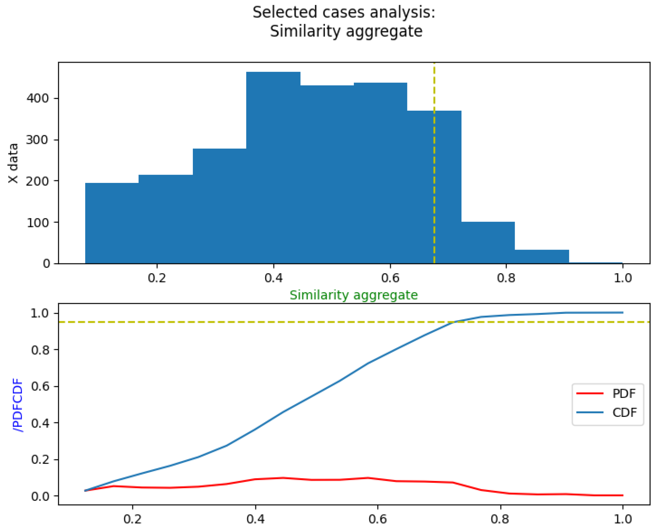
2.4.1. Similarity Functionality

The similarity calculation is a process that is undertaken on the pairs of emergent case data/database case data for the purpose of determining which cases from the database are closest to the emergent one.

The similarity score is broken down into two individual scores:

• Room similarity
• Damage similarity

Each of the individual scores is added to create the similarity aggregate $\left(Similarit{y}_{agg}\right)$.

$$Similarit{y}_{agg}=w_1\times similarit{y}_{room}+w_2\times similarit{y}_{damage}$$

(1)

where $w_1, w_2$ are weighting factors. The factors’ selection is an involved process; a high room similarity weighting factor makes sure that the high factuality data from sensors or crew regarding damaged rooms is given precedence over the damage variables. On the other hand, too high a value degrades the robustness of the comparison if it is based on only one of the two streams of information. In this implementation, values of 0.6 and 0.4 are used, respectively, which is found to satisfy the above rationale.

The similarity scores for the rooms are based on Jaccard similarity. Jaccard similarity measures the similarity between two sets of data and is often used in that function.

$$J\left(A,B\right)=\frac{\left|A{{\displaystyle \cap }}^{ }B\right|}{\left|A {{\displaystyle \cup }}^{ }B\right|}$$

(2)

For the room similarity, the Jaccard similarity is applied straightforwardly. The Jaccard similarity measures the similarity between two sets of data by dividing the size of the intersection of the sets by the size of their union.

In the case of damage, a custom metric was developed. The metric uses a series of functions, each of which is tailored to a specific damage variable and calculates a “closeness” metric ranging from 1 for complete similarity to 0 for complete dissimilarity. The functions are different for each damage variable, as the physical meaning of the damage variables varies. Additionally, each damage variable has a unique weight assigned to it, reflecting its relative importance in the calculation of the damage similarity.

$$Similarit{y}_{damage}={\displaystyle \sum }_{i=0}^{n}S{m}_{va{r}_i}\times w_i$$

(3)

where $n$ is the number of damage variables. Each damage variable also has a custom difference/similarity function that describes what is classified as similar in terms of value difference. For example, two cases of 2 and 2.5 deg heel are considered similar for the heel, but a difference of 0.5 for the survival factor is completely dissimilar.

2.4.2. Retrieval of Cases

The similarity function is applied to all cases to find the cases that are most similar to the emergent case. Each case is then assigned a similarity score based on the similarity function. The resulting database is sorted in descending order of similarity scores.

To reduce computational time, only the most promising cases are considered. A percentile value is used to determine the similarity score cut-off, which shifts based on the distribution of similarity scores. An example of this function can be seen in Figure 2. In the following figures, a histogram is first presented showing the number of cases for each similarity score bin, whilst in the bottom subplot, the Probability and Cumulative Density functions (PDF/CDF) are drawn for the same distribution. Similarly, the same template is used to plot other values, such as the survival factor (SFAC) or heel, etc.

In this case, the 92nd percentile is used as the cut-off for selecting cases. This choice is made because it includes the highly similar cases, while avoiding large clusters of less probable cases. As seen in Figure 3, the higher concentration of high scores shifts the cut-off to a higher similarity score, as expected.

After the selection process, data is extracted from the relevant cases in an appropriate manner. This can include any of the values stored in the database, such as the response of the vessel to the damage (described by the damage variables).

Additionally, the probability of correctly predicting the case can also be incorporated into the analysis. The database already contains the a priori probability of each case in the form of the “p factor”. Some cases are more probable to occur due to the distribution of damages considered in SOLAS. To incorporate this knowledge into the similarity factor, Bayesian inference is used to form a probability that the specific case is taking place. This is achieved by using Bayes’ rule, similar to a sensor fusion problem. Bayes’ rule lies at the heart of most data fusion methods and provides a means of making inferences about the state, x (in this case, which case from the database is occurring/evolving), based on an observation, z, (the similarity metric). The joint probability is obtained using Bayes’ rule [36].

$$P\left(x|z\right)=\frac{P\left(z|x\right)P\left(x\right)}{P\left(z\right)}$$

(4)

The conditional probability $P\left(z|x\right)$ serves the role of a sensor model, as it describes the likelihood that a specific z observation is obtained conditioned on the state of x. This value has been evaluated for each case (x) by using the “sensor” similarity score applied to variables of x. This term is also denoted as the likelihood function in the literature. The denominator, $P\left(z\right)$, is the marginal probability and is used to normalize the posterior probability, $P\left(z|x\right)$ by ensuring that the sum of all conditional probabilities sums to 1. Finally, $P\left(x\right)$, contains all prior beliefs on the state of x, irrespective of observation. The a priori distribution is the p factor based on the SOLAS formulation.

According to the above formulations, the probability of a case being the one really happening is given as the posterior probability $P\left(x|z\right)$. Where $P\left(x|z\right)$ is:

$$P{\left(x|z\right)}_i=C\times Similarit{y}_{ag{g}_i}\times pfa{c}_i$$

(5)

where:

$$C=\raisebox{1ex}{$1$}\!\left/ \!\raisebox{-1ex}{${{\displaystyle \sum }}_{i=0}^{n}P{\left(x|z\right)}_i$}\right.$$

(6)

where $n$ is the number of cases in the database.

In conclusion, the prior belief contained in the a priori distribution of probability (p factor) helps to give more weight to cases that are more frequent and less weight to rare cases. This is useful when the sensing accuracy is low, as the prior belief becomes the main source of information for the algorithm.

2.4.3. Adaptation

The result of the previous step is now a probability density function (that integrates to 1) for not only the similarity of the cases, but also for every value linked to the cases. For example, see Figure 4 and Figure 5 below:

The yellow line in the case of variables is defined by the mean value and the corresponding cumulative density function (CDF) of that value in the bottom graph. Note that the average extracted here assumes that all the selected cases are equal in weight. In

Table 3. Output prediction types.

Name	Sample	Method
Simple average	Selected cases (by percentile similarity cut-off)	$\frac{{{\displaystyle \sum }}_{i=0}^{n}va{r}_i}{n}$
Weighted similarity average	Selected cases (by percentile similarity cut-off)	$\frac{{{\displaystyle \sum }}_{i=0}^{n}va{r}_i\times Similarit{y}_i}{{{\displaystyle \sum }}_{i=0}^{n}Similarit{y}_i}$
Weighted posterior probability average	Selected cases (by percentile similarity cut-off)	$\frac{{{\displaystyle \sum }}_{i=0}^{n}va{r}_i\times P{\left(x|z\right)}_i}{{{\displaystyle \sum }}_{i=0}^{n}P{\left(x|z\right)}_i}$
Top case	Top case by similarity	Top case feature value

the different methods of extracting a singular value as the prediction are found.

Below is an example with a randomly generated case (Figure 5) that demonstrates the different prediction methods. The similarity aggregate can be used instead of the probability for “an uninformed a priori” prediction (see

Table 4. Example of different predictions relevant to Figure 5.

Name	Value
Simple average	0.96
Weighted similarity average	0.9669
Weighted posterior probability average	0.990
Truth	1

).

The simple average will be less specific and more conservative. The same effect is replicated if the percentile selected is lower or higher. A higher percentile will narrow the scope to the most similar cases, while a lower one will encapsulate more cases, thus being more conservative and less specific.

2.5. Machine Learning Fundamentals

Machine learning (ML) is a field of computer science that uses specialized algorithms, techniques, and processes for generating solutions to complicated problems that are hard to tackle with conventional programming approaches. Most importantly, in machine learning the programmer does not design the program to solve a problem explicitly in predefined steps, but instead sets up a framework of rules and functions that can achieve that by “learning”. This “learning” is possible given a labelled dataset that essentially contains examples of input-output pairs that the algorithm then “learns” to reproduce for new input data and provide correct results. This is called supervised machine learning. ML algorithms can solve many complex problems using this generic approach [37].

2.5.1. Performance Metrics

There are several metrics that can be used to quantify the performance of a machine learning application. Classification and regression problems both have specific metrics that can apply. While several of them were used to create those models, there will not be an extensive discussion on their formulation or on other metrics that were not used. Similarly, the implementation of the ML process pertains more to computer science, and as such it will not be discussed extensively, nor is the author claiming that it is properly optimized. The main objective is to show how this approach works and to demonstrate its potential for this particular problem. The metrics as presented below are formulated and used as part of the Python scikit-learn (sklearn) library [38] for the purposes of evaluating each trained model.

2.5.2. Classification

In classification a class has a binary nature, hence the performance metrics are adapted to depict this reality.

2.5.3. Accuracy

Accuracy is a simple metric that is defined as the sum of correct predictions divided by the total number of predictions. For example,

$$\begin{array}{c}\left[\begin{array}{c}Predictions\\ Truth\end{array}\right]=\left[\begin{array}{cccc}1& 1& 0& 0\\ 0& 1& 0& 0\end{array}\right]\\ Accuracy=\left[\begin{array}{cccc}0& 1& 1& 1\end{array}\right]=\raisebox{1ex}{$3$}\!\left/ \!\raisebox{-1ex}{$4$}\right.\end{array}$$

(7)

In the above example, there are matching predictions with truth in three cases out of a total of four, hence the score comes out to 75%. It is an easy way to see if the classifier is working and how good it is at correctly identifying the class. However, it can be misleading on its own, especially in cases where the classes are imbalanced. For example, if 90% of the data is positive, then a classifier that only returns positive data will be accurate at 90%.

2.5.4. Precision

Precision is given by:

$$Precision=\frac{Tru{e}_{pos}}{\left(Tru{e}_{pos}+Fals{e}_{pos}\right)}$$

(8)

where $Tru{e}_{pos}$ is the number of true positives and $Fals{e}_{pos}$ is the number of false positives. Positive and negative here refer to the possible states of the binary classifier. The precision metric provides insight into the classifier’s ability to not generate false positives. This metric can be very important depending on how the problem is formulated. In this present application, the positive label is given to correspond to a survival factor of 1, hence a false positive would mean that a dangerous prediction is returned. The ideal value is 1, while the worst is 0.

2.5.5. Recall

Recall is a metric that captures the ability of the classifier to find all the positive samples. It is given by:

$$Recall=\frac{Tru{e}_{pos}}{\left(Tru{e}_{pos}+Fals{e}_{neg}\right)}$$

(9)

where $Fals{e}_{neg}$ are the number of false negative predictions, or predictions that are positive but are misclassified. The ideal number is once again 1, and the worst is 0.

2.5.6. F1 Score

The F1 score, also known as the F-score or F-measure, combines precision and recall in one metric by taking their harmonic mean. It is useful to compare two different classifiers by evaluating precision and recall together.

$$F1=2\times \frac{\left(Precision\times Recall\right)}{\left(Precision+Recall\right)}$$

(10)

Again, the best value is 1 and the worst is 0. The F1 score is useful in cases where the accuracy is not as robust. This is primarily for imbalanced datasets that were discussed. Furthermore, it can better capture the difference in consequences of a false positive/false negative. For example, for a cancer recognition application, a false negative is many times more costly than a false positive (considering that follow-up investigations will reveal it to be false).

2.5.7. Regression

Regression performance metrics revolve around the idea of fitting a curve to a cloud of data points and associated metrics that can be generally found in mathematics and statistics.

2.5.8. $R^2$ Coefficient of Determination

In statistics, the coefficient of determination is routinely used to explain how well the statistical model replicates the observed data points. Similarly, in ML it captures how well the model can predict the data given, and as such a high value is sought.

2.5.9. Mean Absolute Error

Mean absolute error (MAE) is also found in statistics, and captures the average of the absolute errors for pairs of prediction-ground truth data.

2.5.10. Root Mean Square Error

Root mean square error (RMSE) or root mean square deviation is another tool very commonly found in statistics that once again captures errors, but in contrast to MAE, each error has a different effect, especially for the outliers.

2.6. Machine Learning Implementation

Machine learning, as introduced earlier, is an approach that has been used in this case to get similar results to the case-based approach. More specifically, using ML, models are trained on the data in the database and then used to extract predictions as in the CBR approach.

The implementation of ML methods happens in parallel to the CBR approach in the same script, relying on the Python library, scikit-learn [38]. The objective is to utilize the information found in the dataset to provide predictions for an emergent case. In contrast to the CBR approach, many of the functionalities of how this happens are not distinct, and are defined by each model’s internal logic as well as pre- and post-processing steps.

The steps followed for each ML implementation are:

• Provide database of cases (pre-processed).
• Select features from the database and the target feature (objective to be predicted).
• Select a machine learning model, e.g., RandomForestClassifier.
• Choose whether to binarize the target feature.
• Choose the threshold for binarization.
• Choose whether to standardize the data.
• Search for best hyperparameters (grid search).
• Train model.
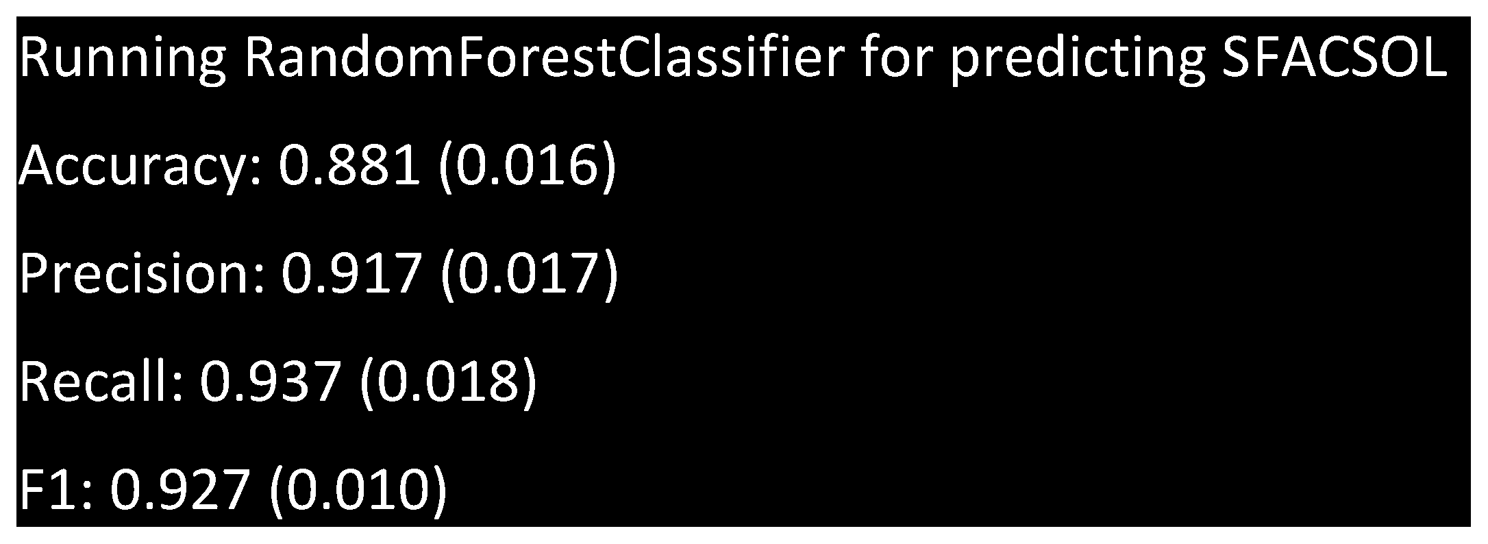
• Perform K-fold cross validation and display mean and std. of performance metrics ($r^2$, accuracy etc.).

Initially, the script manages the steps of splitting the dataset to train and test the sets. The split used is 0.3, meaning 30% of data is kept for the testing/validation step. It is common practice to take random slices of the data for training and testing to avoid overfitting and to get accurate validation results. The process of cross-validation goes one step further. In cross-validation, the splits of train-test data are done multiple times each time, measuring the performance of the model. After a number of runs, the data can be collated.

The model is trained on the data after the split is done correctly.

Lastly, the trained model passes through an evaluation function where several of its performance metrics are computed, as well as other outputs. Some are also printed as below (Figure 6):

This process is repeated for a large selection of relevant ML models, and the best are selected automatically each time they are trained. See Section 3.

Note that the values are returned as the mean and the standard deviation in parentheses since the model is evaluated across all folds or splits of data (typically 10).

2.7. Classification

There are no features of the damage cases that fit the description of a binary classifier. However, with some adjustments several can be created. For example, the most important classifier feature that was adapted is the survival factor. While normally SFAC ranges from 0 to 1, the extremes are what is seen most of the time. In addition, values lower than 1 but not zero usually represent a “degraded” survival, usually one with a large heel angle. Hence, cases with a value larger than 0 are generally survival cases, albeit marginal ones. Consequently, by choosing a threshold value in the range of 0 to 1 and then binarizing the SFAC, it is converted to a classification output. For example, considering 0.7 as the threshold, then all entries with a value higher than 0.7 will become 1, and those lower will become 0. A high threshold will generate more non-survival cases from the marginal ones, while a lower one is the inverse of this. The threshold value used is 0.7 in the code. A “binarizer” function carries out the procedure across the database.

Another possible classification target is a new feature named “Capsize” that is generated by interpreting the data already found, such as heel and trim, etc.

2.8. Regression

Regression refers to the direct prediction on a continuous variable. There are several possible target features with different ranges. For example, the heel is quite important, as is the range of positive stability and GZ. SFAC is also a continuous variable that can be predicted. A very similar approach is followed by first comparing the models or regressors. Of course, the continuous nature of the data changes several ways of approaching the regression problem compared to the classification.

In this study, the performance is basically evaluated similar to the way of fitting a curve to data. The model attempts to explain the true data as a function of other data. A successful regression model will have a high coefficient of determination or $R^2$, and low errors between the predicted and measured data points.

3. Results

The models are divided into classification and regression models, and each are trained in turn, and the best model is kept and used for the predictions. This process takes approximately 13 min and needs to be run only once, as the models are automatically saved. The training regime uses 10-fold cross validation on the basis of 70–30 % training-test/validation data. For deployment, the model should then be trained on the whole dataset available. The SFAC classifier can evaluate 40 sets of input data per second, thus completing a standard normalized set of 400 cases per given input data every 10 s.

3.1. Classifier Comparison

In order to compare the performance of several trained models, a function was developed to compare their results. The graph in Figure 7 visualizes the classifiers’ predictions by plotting the data points with a coloured background. Each data point represents a case, and its colour corresponds to the SFAC value of the case (blue for 1 and red for 0). The location of the data points is based on the two most important features: length an location, as determined by analyzing the feature importance of the models (see Figure 8). For plotting, only these two features can be used, as the plot is 2D.

Figure 7. Classifier comparison: The bullet points represent known data, while the painted background displays the model predictions. The X axis is length and the Y axis is location. Only these two features are shown here, while the models use additional ones. The accuracy of each model can be found in

Table 5. Accuracy scores of the classifier models tested.

Model	Accuracy Score
Nearest Neighbors	0.82
HistGradient	0.84
Linear SVM	0.81
Neural Net	0.83
AdaBoost	0.85
Naive Bayes	0.81
RBF SVM	0.81
Decision Tree	0.84
Random Forest	0.83
QDA	0.82
Stacked model	0.83

.

Figure 7. Classifier comparison: The bullet points represent known data, while the painted background displays the model predictions. The X axis is length and the Y axis is location. Only these two features are shown here, while the models use additional ones. The accuracy of each model can be found in Table 5.

The background of the graph represents the predictions of each model, with the intensity of blue and red hues indicating a higher or lower probability of predicting 1 or 0. The accuracy score of each classifier is also shown at the bottom right of the figure, with the stacked classifier being a combination of all the other classifiers. In general, all classifiers have similar performance, as does the stacked model.

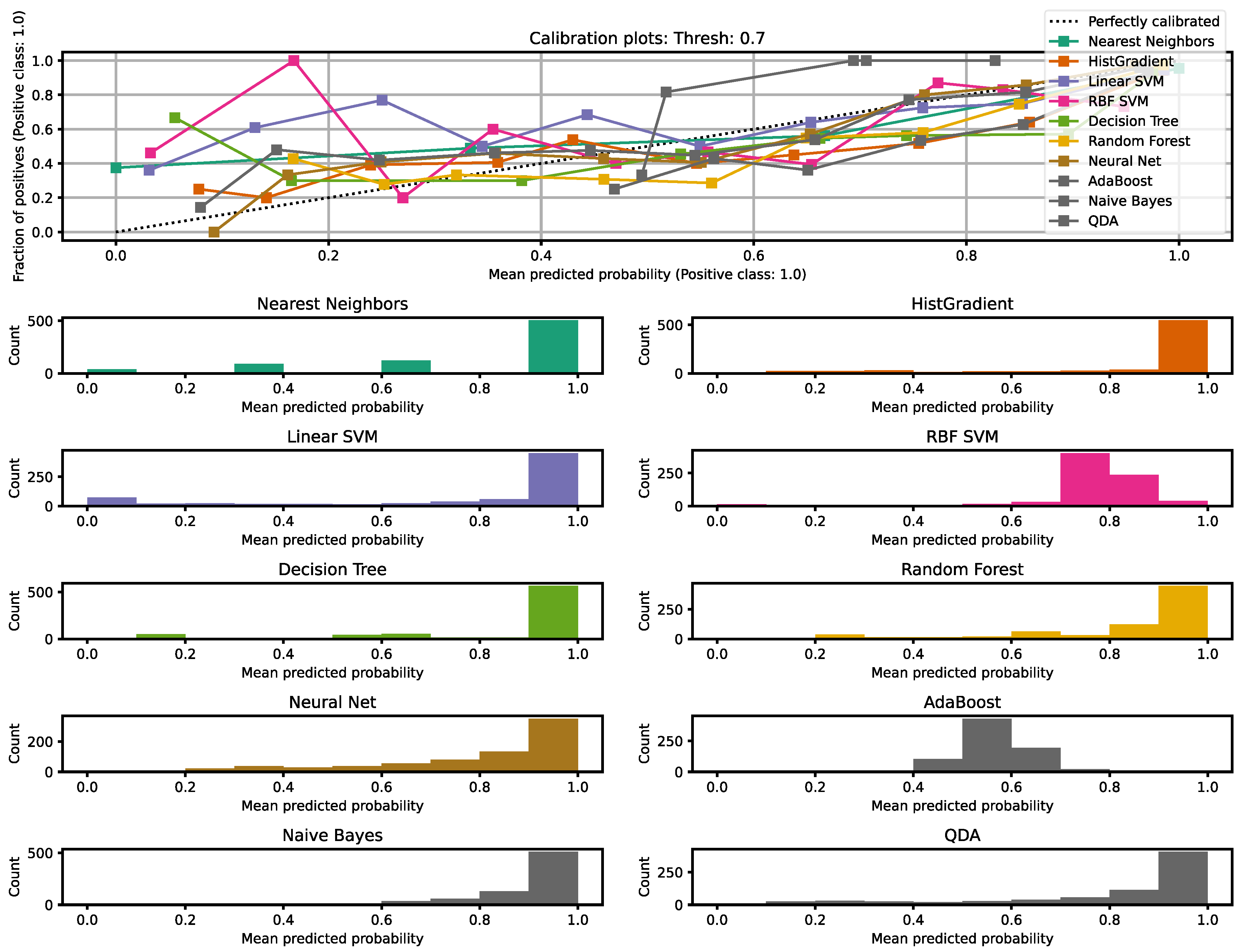
3.2. Calibration of Models

The calibration of the models was performed to adjust the output probability to match the ratio of positive classes in the relevant set. The calibration process was visualized using the calibration curve, which plots the mean predicted probability against the fraction of positive classes. The goal is for the data points to lie on the y = x diagonal. Figure 9 and Figure 10 show the uncalibrated and calibrated calibration plots for all classifiers.

Receiver Operating Characteristics and Discrimination Threshold

A useful way to visualize the effect of differing discrimination thresholds can be afforded by a graph known as the receiver operating characteristic graph (ROC), see (Figure 11).

The result for the default 0.5 threshold for the calibrated classifier is printed below (Figure 12):

3.3. Regressor Comparison

A comparison of various regression models was conducted to determine the best model for predicting heel, GZMAXR, and others. The comparison was performed by fitting the models to the same data and plotting the results. In these plots, the perfect fit is represented by a diagonal line, where the predicted value equals the measured value, with the predicted values on the y-axis and the true values on the x-axis.

Among the regression models, the best performers were found to be Gradient Boosting and Random Forest. Although a stacked model combining all the individual models was also computed, it was not found to be superior to the individual models. After careful evaluation, the Gradient Boosting model was selected as the final model for predicting heel, due to its high $R^2$ and low mean absolute error (MAE) relative to the other models.

The same model was also found to be the best for predicting GZMAXR & heel (Figure 13 and Figure 14).

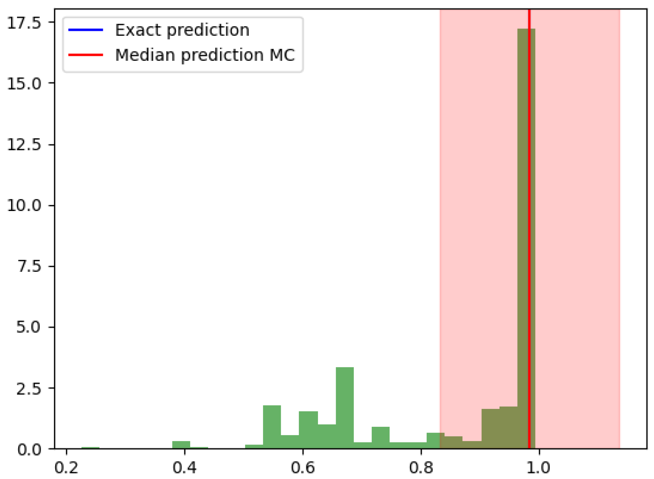
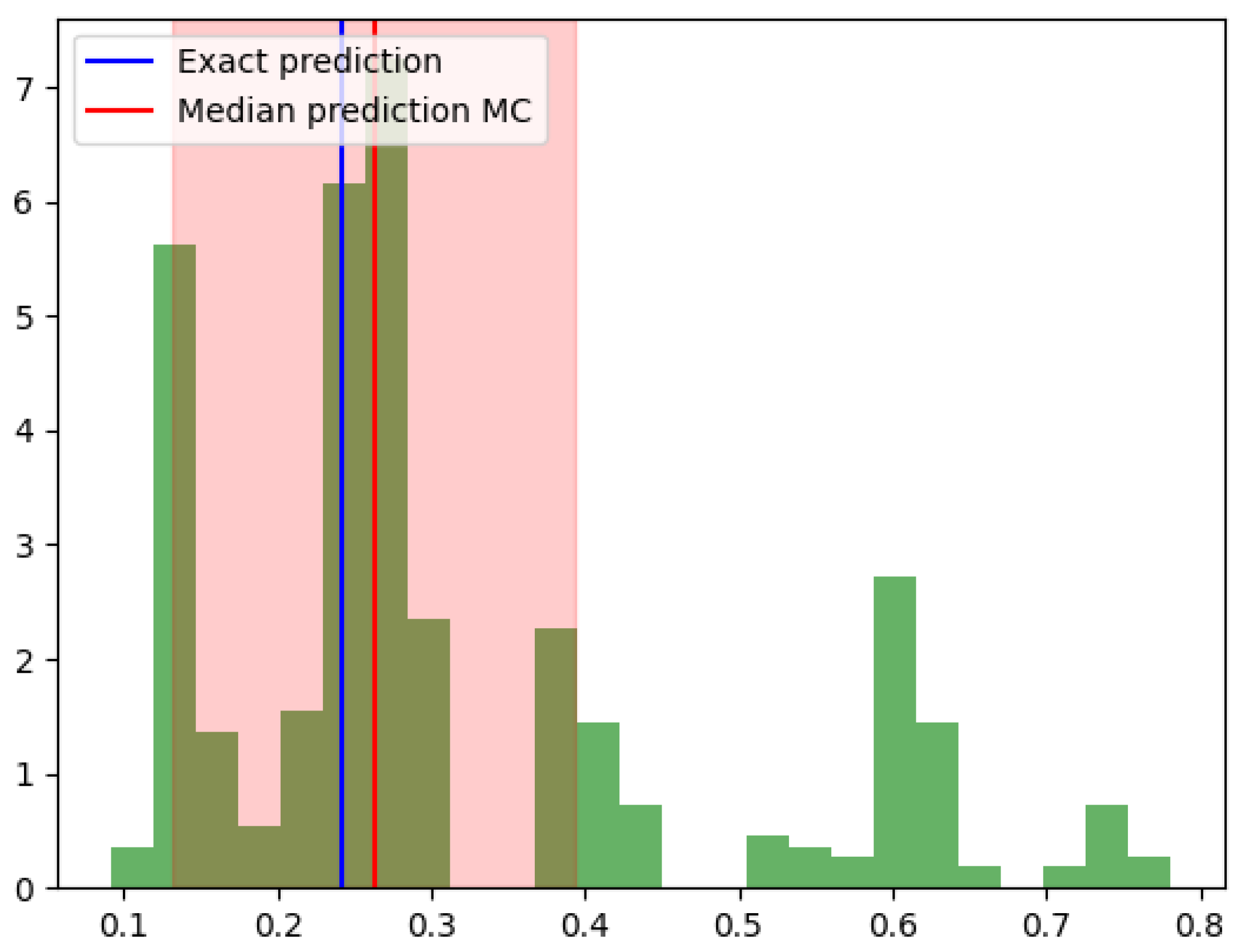
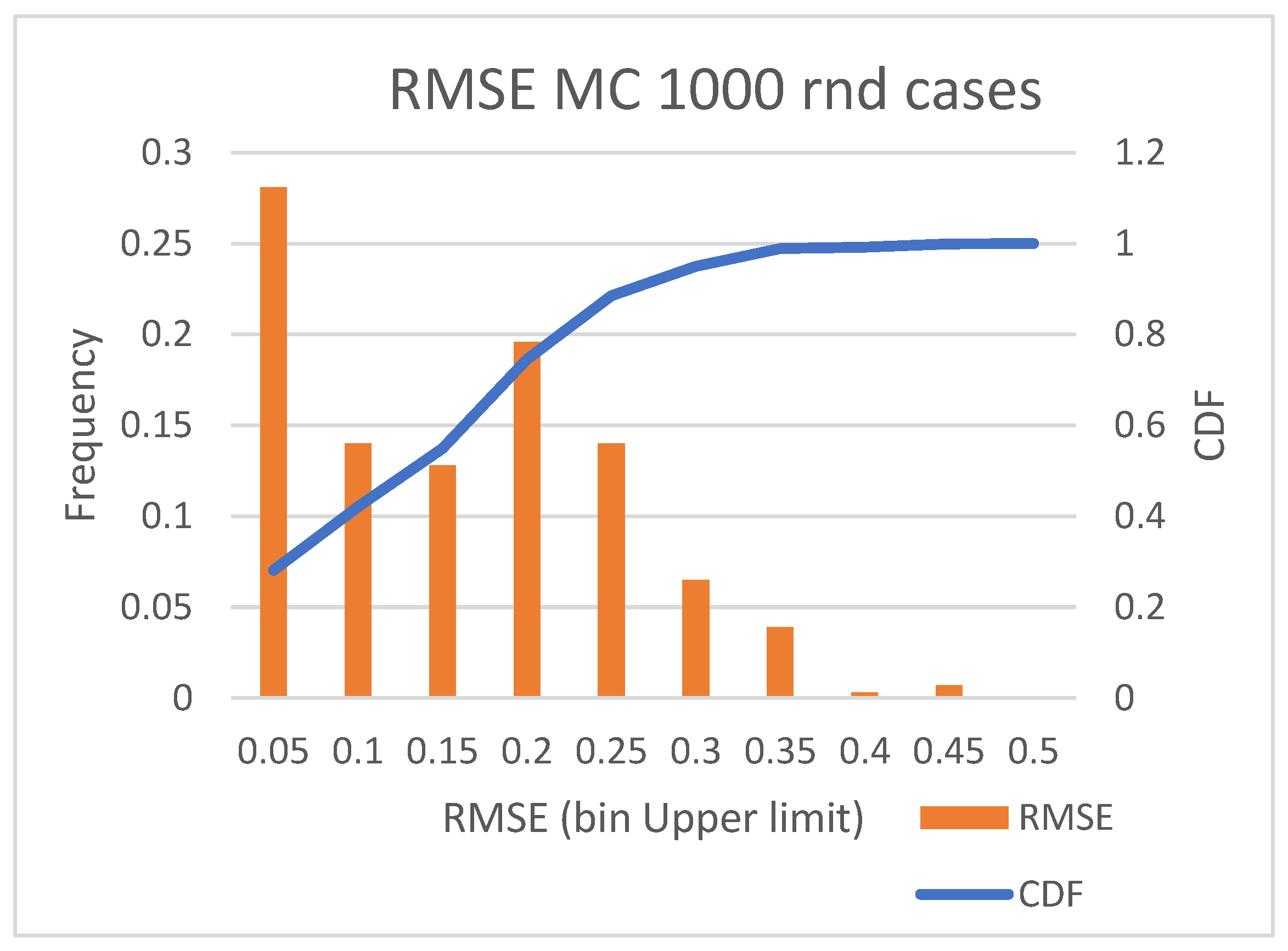
3.4. Uncertainty Quantification for Input Variables

A sensitivity analysis was performed in order to assess the effect of uncertainties in the input variables on the predictions of interest. The input variables of concern are the damage variables, such as the length and location of a breach, which are critical for the task at hand.

The uncertainty of these damage variables is quantified using a normal distribution centred around the measured value. The standard deviation, which reflects the degree of variability of the measurement, is determined for each variable based on its inherent characteristics. For example, the location of the damage is discretized into tenths of the ship, and a measurement of 4 would result in a normal distribution with a mean of 4 and a standard deviation of 0.7. This deviation was chosen to capture the probable measurements that could be obtained from a human observer.

In the case of the length of the damage, the deviation of 1.5σ corresponds to 87% of the measurements of a normal distribution. It is important to note that the standard deviations were selected based on logical considerations, but without the use of specific data.

It is worth mentioning that due to the discrete nature of the values, the resulting density bars may not follow a normal distribution (Figure 15 and Figure 16).

To analyze the impact of the uncertainties in the damage variables on the prediction, a Monte Carlo simulation was performed in the study. Initially, 400 instances were randomly selected from the normal distributions of each variable and shuffled into a list of cases. These cases are essentially possible permutations of the variable distributions shown above, and were then evaluated using machine learning models to obtain predictions.

Additionally, the original case was also evaluated and considered as the “exact” prediction. The results from the 400 predictions and the exact prediction were plotted to visualize their distribution.

This Monte Carlo simulation provides a robust assessment of the effect of uncertainties in the input variables on the prediction, allowing for a comprehensive understanding of the potential outcomes and their associated uncertainties. The results of the simulation can be used to make informed decisions and to assess the robustness of the prediction models. The following graphs contain 400 random cases evaluated in that way (Figure 17, Figure 18 and Figure 19).

In the Monte Carlo simulation described above(Figure 17), the results indicated that most of the data was concentrated between 0.1–0.4, and that this region also contained the exact value. The spread of the density of the data provides an indication of the uncertainty in the prediction. In this particular case, the spread of the data was relatively low, as indicated by the low standard deviation.

Furthermore, the mean and exact predictions were found to be close, suggesting that the exact prediction was relatively robust in this scenario, and was not greatly affected by the uncertainties in the input data.

In Figure 18, the spread is even lower, and the mean and exact predictions coincide even more. The shaded area is also narrow, meaning that the uncertainty is low.

Figure 19 is an example where there is a large spread of values for the prediction. This variance suggests high uncertainty in the prediction as well. The shaded area also has a large range. In this case, the uncertainty of the prediction is high.

It is obvious that each case can have a different uncertainty associated with it. In order to evaluate the general effect that input variable variation can have on the end result, a Monte Carlo simulation was carried out. The same 400 permutations on the distribution of input variables are computed for 1000 random cases picked randomly from the database. The prediction on SFAC is used to compare the results. For every case, the percentage as well as the root mean square error of the 400 predictions against the exact prediction on the case without transformation are kept, see Figure 20 and Figure 21. The standard deviation is also kept, as is the coefficient of variation. The purpose of this is to generate a histogram and a CDF showing how the end prediction is affected across the cases of the database. The prediction is done through the ML models generated and calibrated according to the previous chapter.

This process is quite computationally intensive, as there are a total of 401,000 predictions that need to be made, as well as the generation of random input variable tables.

The resulting data is plotted as histograms to better visualize the density of the shift.

The results of the Monte Carlo simulation reveal that the methodology and input variable discretization are robust, as the expected variation in accuracy in the input variables does not significantly affect the prediction accuracy compared to the exact prediction. The ML models also appear to not be overfitting to the database cases, as new cases around those cases are evaluated similarly. The 90th percentile of the root mean square error is 0.25, meaning that in 90% of the cases the error is less than 0.25. The percentage error histogram is also plotted, but it should be noted that care should be taken when interpreting the results, as the same percentage error can have different implications for the different values of SFAC predicted.

4. Discussion

A high-level overview of the methodology presented is found in Figure 1. Below are some examples of how the predictions are returned for various variables.

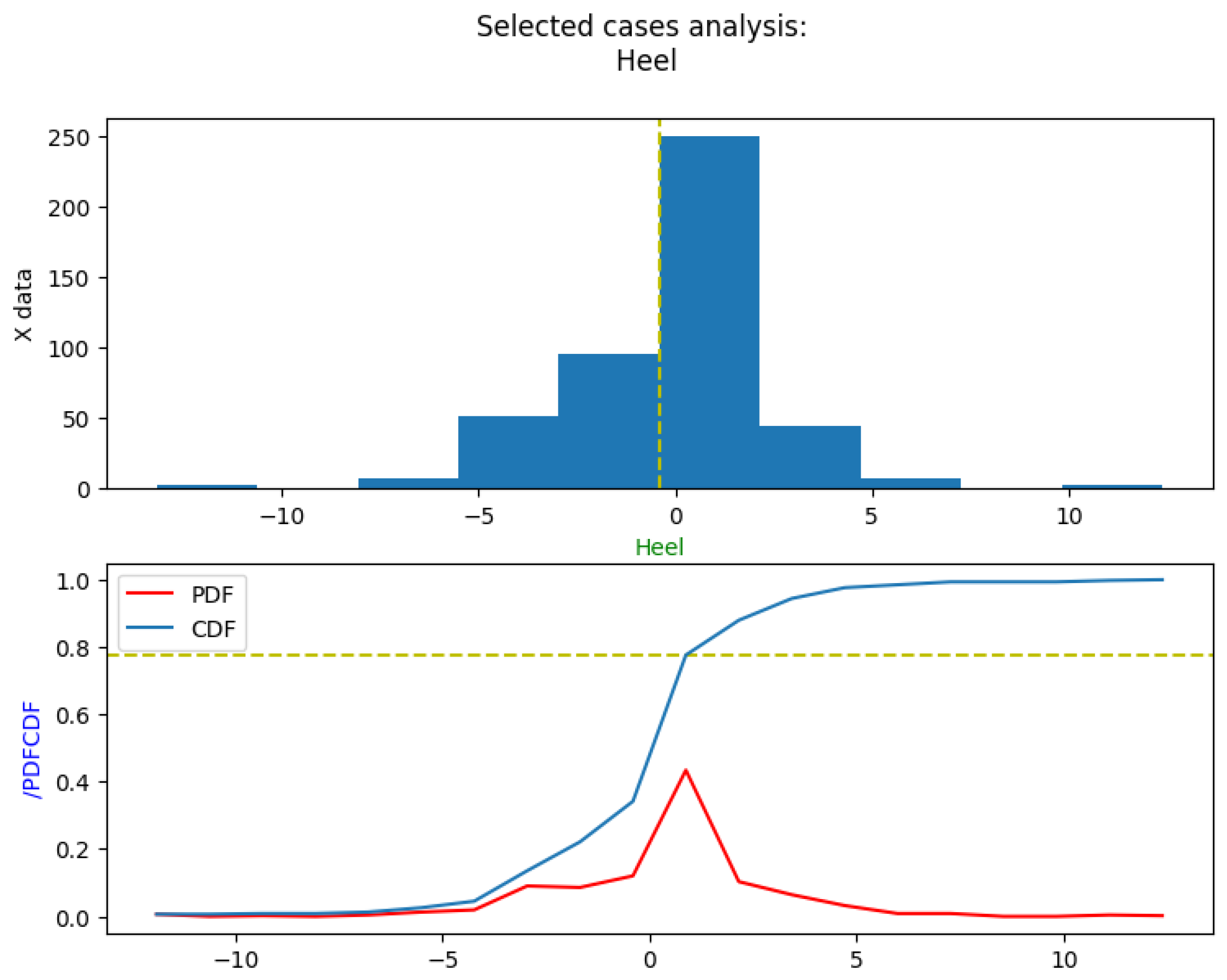
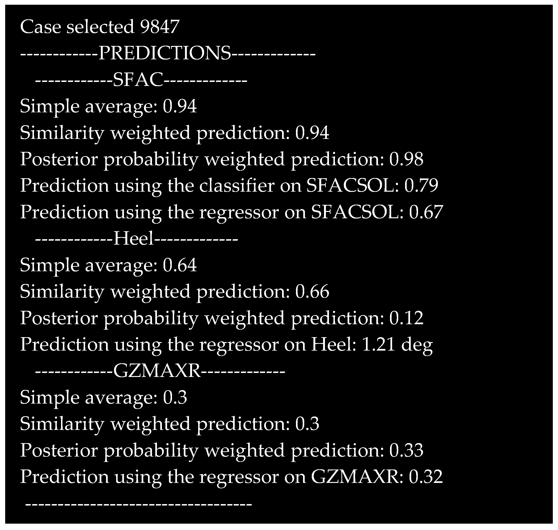
4.1. Predictions of Selected Variables

The predictions are printed along with the rest of the output from other models, and the CBR approach is in the following format (Figure 22 and

Table 6. Tabulated results for case 9847.

	CBR Approach		ML	Truth
	Similarity weighted predicted	Posterior probability weighted	Machine learning prediction
Heel	0.66	0.12	1.21	−0.02
GZMAXR	0.3	0.33	0.32	0.29
SFAC classifier	0.94	0.98	0.79	0.98
SFAC continuous	0.94	0.98	0.67	0.98

).

The above process can be followed for all features found in the database. Several cases were evaluated in this way in order to validate the methodology.

4.2. Prediction on Time to Capsize

The survival factor is an obvious prediction; however, the prediction of the time to capsize is also very important.

Due to the small scale of the database, TTC times cannot be evaluated directly. Note that since the TTC is based on data that are 30 min long, an adjusted TTC is used to expand the range of predictions instead. This adjusted TTC is the result of multiplying the TTC with two exponentials to the power of the predicted survival factor. In short, the survival factor is used to extend the range of the TTC artificially based on the idea that a high survival factor indicates a safe case (TTC $\to$ inf), while a lower survival factor indicates a sinking or capsizing case.

$$TT{C}_{adj}=\raisebox{1ex}{$a\times TT{C}_{ind}\times \left(e^{b{S}_{fac}}+e^{c\left(S_{fac}-0.7\right)}\right)$}\!\left/ \!\raisebox{-1ex}{$3600$}\right.,hours$$

(11)

where $a=0.45, b=1.5, c=12$. The function can be visualized below (Figure 23).

Following the logic of the function, high TTC values basically denote survival. The indicated TTC is taken directly from the regressor for predicting TTC. If a case has no capsizing in 30 min of simulation, then the TTC is returned as 3600 s (1 h).

Using the above formulation, the CBR and ML methodologies can be made to produce TTC predictions.

Several scenarios of damage were created and simulated through the inputs to demonstrate the code functions and performance.

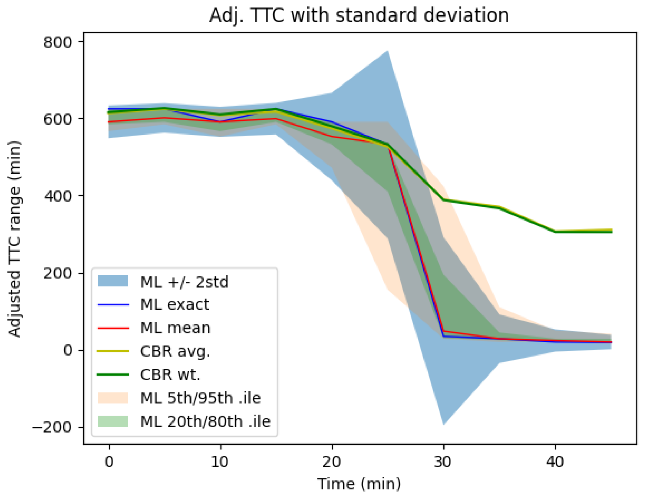
4.2.1. Rapid Capsizing

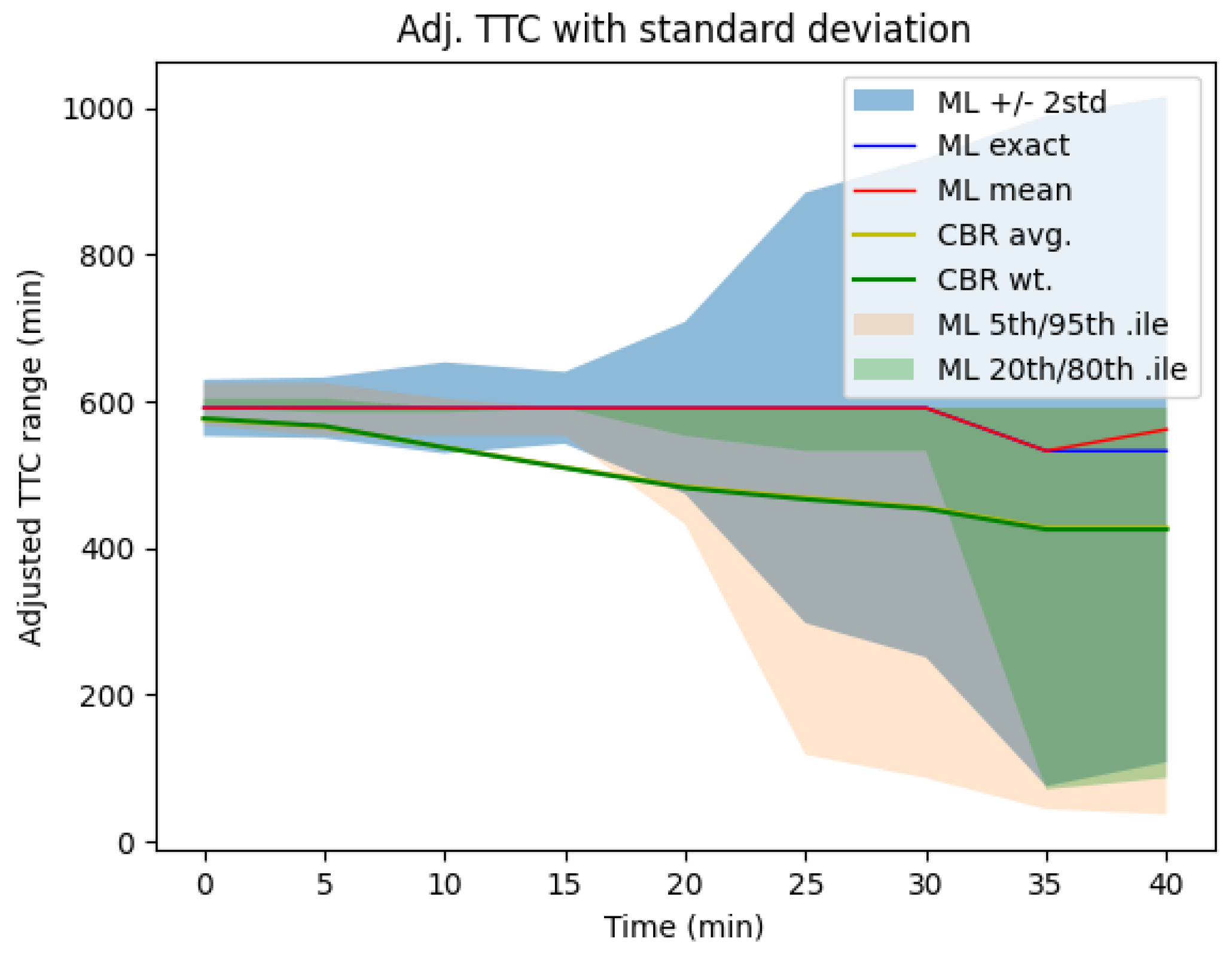
In this damage scenario, input data is provided 10 times. Initially, the damage is thought to be small and localized, which is proven to be false as time passes. This is reflected only in the data provided by sensors or crew (

Table 7. Ten damage updates given sequentially.

Index	Length	Pen	Z_Centre	Z_Height	Location_Side
1	5	1	2	2	−5
2	5	2	2	2	−4
3	5	2	2	2	−6
4	7	1	2	2	−5
5	15	1	2	3	−5
6	21	1	2	3	−5
7	30	2	2	3	−6
8	35	3	2	3	−6
9	40	3	2	3	−6
10	53	3	2	3	−6

).

Generally, as time passes, the real extent of the damage becomes clear, with the last update corresponding to the damage variables stored in case #6907 of the numerical simulation database for flooding. The rooms that are found to be flooded are also given in a separate table. This information is used by the CBR methodology to find similar cases. Many cases share similar rooms, so an increase in the number of passed rooms invariably makes the prediction more accurate, as less and less cases share the same rooms. The rooms passed do not influence the ML methods.

From the two data streams provided, it is clear that as time passes the accuracy is expected to rise. In the first five sensor updates, the rooms passed are found in multiple cases, many of which are survival cases. Starting from the sixth update, the rooms involved point more and more towards a rapid capsize case (#6907). However, the total amount of rooms is never passed as sensor input, as can be expected in a real case that spans large spaces. The code then prints and updates the following plot with the predictions from the CBR and ML methodologies in real time (here presented at the last time step, see Figure 24).

The histograms (see Figure 25) also provide valuable information on the distribution of the CBR cases. Up to update #6, a significant number of cases had high TTC values, and at update #7 the new data reshapes the landscape, now giving much higher density in the low region. It is becoming more evident that there is roughly an equal chance of either capsizing or surviving.

After update #10, which includes the best information found, the predictions from all sources converge substantially. See above how the CBR methodology basically converges to a substantially low TTC. Furthermore, the “noise” or variability introduced in the ML method seems to have little effect on the result, as similar cases also have similar outcomes, and the deviation in the 400 random cases evaluated by the ML method is very low, see Figure 26. The confidence bands are also tight around the ML median.

Finally, two out of three metrics used here suggest a TTC of 20–30 min, with enough data to support the accuracy of these predictions. The CBR approach is largely affected by other survival cases, and thus has a higher weighted value. It is also useful to note that any safety system should inherently be conservative, and hence the appearance of several possible cases that lead to sinking would require a fast response on board in order to minimise the perceived risk.

In the case of a rapid capsizing, it is very important to quickly identify the situation as critical so that the evacuation process or other active crisis management measures (e.g., intentional grounding) can be taken. It was demonstrated how such an event would be dealt with in the case above.

4.2.2. Slow Capsize

Case #1918 is used to demonstrate a slow capsize case, see Figure 27. Case #1918 is evaluated in the time domain, showing a large angle of heel but no capsize in 30 min of simulation. In that situation, this case can easily go either way if external forces are added, etc. It was also demonstrated here how the distribution of damages can be used even when the exact prediction may be favourable.

Due to the low criticality of the damage information given, the initial 5–6 ML predictions suggest a non-capsize case with high confidence (narrow deviation band). Here, the decision maker should focus on the uncertainty of the indicated large TTC and the delicate balance between survival and capsize/sinking, as well as the top cases having high similarity but also low TTC times. This data should indicate that action is definitely needed and that an orderly evacuation is possible. This decision can also be strongly influenced by the estimated time to exceed the maximum heel (and trim) angle that is compatible with the safe deployment of LSAs (e.g., 20 degrees).

The scenarios shown above demonstrate how the crew onboard can quickly get an evaluation of relevant data without needing to consult any other tool. Traditionally, seafarers would have to retrieve and examine the trim & stability booklet or a special damage stability booklet, where they would try to use precalculated aids, revolving around the ideas of reserve buoyancy and final floating position for continuous damages. Instead, using the proposed methodology, the crew is only responsible for providing the input variables while the scope of the damages is as broad as the database. If the present methodology was to be adapted directly, that would mean the input of damage characteristics in the scales presented in Table 1. and specifically, those of length, location, penetration, height, and center height. The inclusion of flooded rooms is optional, but greatly improves the CBR prediction. In mere seconds the models can compare the emergent situation with the precalculated ones and immediately display information that can inform decisions in an uncertain environment. It has been shown, for example, how uncertainty is also displayed as an output and should therefore also influence decisions. Most importantly, the models do not need to have been trained on the same case that is happening in order to provide good results. The approach is also modular; it can include more and more cases, but is also robust to uncertainty; as shown in the Monte Carlo simulation.

5. Conclusions

The authors have presented an extensive methodology, integrating two reasoning methods that build upon pre-calculated databases. Both parts of the methodology have been processed and evaluated to be valid in real-time evolutions of damage scenarios. For example, the variable inputs are easily obtained with low complexity and technology means. The input considered is adjusted to represent the expected sources of information during a casualty, namely crew optical assessment. The uncertainty introduced due to the data type and source has also been computed and represented to inform any prediction of the presence of uncertainty. The methodology has been shown to produce logical results with good results in predicting important variables, especially the survival factor. The representation of the prediction is also discussed, as is how important information can be extracted from the multitude of data points provided. Finally, the two methods are shown working in parallel; both provide similar results, and their comparative advantages have been discussed.

The application of machine learning or other reasoning systems in damage stability should be investigated further as a real-time solution that is able to provide a dynamic risk assessment that is useful and lacking in most ships. In addition, and in contrast to other solutions, the relative simplicity of installation and good, robust results further promote this methodology. This implementation does not require high-quality data fed from sensors that will need to be installed, or especially powerful computation, although it can benefit from their presence. A large part of the methodology’s success rests on the extent and depth of the pre-calculated damage cases that will need to be run once for each vessel. Hence, their computational cost can be acceptable.

The contrast of the methodology presented with the largely static and inflexible damage stability tools afforded in most cases is stark; even with lower accuracy, the reasoning afforded by computational models using vast databases is orders of magnitude better than human intuition or the evaluation of singular data streams or perceptions. Weather, non-continuous damages, actual loading, and others can all be captured in this database-based approach. This increase in fidelity does not come at the cost of crew resources, as the information required is simple and can be directly supplemented by sensor data.

Finally, as part of a decision support tool [39], this methodology can provide valuable information regarding the predicted evolution of a flooding casualty that can be used to further inform decisions around active measures, evacuation, or other consequential actions that the crew will need to take in a high-stress, low-information situation. This integration with other tools has been carried out in project SafePASS, creating a computational framework that integrates data from various systems that comprise the dynamic environment surrounding an evacuation.

As a final note, it is clear to the authors that there are various aspects of the methodology presented that can be greatly enhanced. A larger database containing new data would be very worthwhile in enhancing and extending the capabilities of the trained models. Integrating other logic processes can also be very worthwhile; for example, a hydraulic “connectivity” model could independently predict which rooms are expected to be flooded without needing sensor data. Lastly, improvements regarding the model formulation, setup and interaction can also improve the performance of the entire method without considerably increasing the computational cost.

References

1. Kolodner, J.L. An Introduction to Case-Based Reasoning. Artif. Intell. Rev. 1992, 6, 3–34. [Google Scholar] [CrossRef]
2. Agnar, A.; Plaza, E. Case-Based Reasoning: Foundational Issues, Methodological Variations, and System Approaches. AI Commun. 1994, 7, 39–59. [Google Scholar] [CrossRef]
3. Norwegian Safety Investigation Authority Part Two Report on the Collision between the Frigate ‘Helge Ingstad’ and the Oil Tanker Sola Ts Outside the Sture Terminal in the Hjeltefjord in Hordaland County on 8 November 2018. 2018. Available online: https://mtip.gov.mt/en/Documents/MSIU-by-other-countries/2021_05.pdf (accessed on 10 December 2022).
4. Papanikolaou, A.; Spanos, D.; Boulougouris, E.; Eliopoulou, E.; Alissafaki, A. Investigation into the Sinking of the Ro-Ro Passenger Ferry Express Samina. In Proceedings of the 8th International Conference on the Stability of Ships and Ocean Vehicles, Madrid, Spain, 15–19 September 2003. [Google Scholar]
5. Jasionowski, A. Decision Support for Ship Flooding Crisis Management. Ocean Eng. 2011, 38, 1568–1581. [Google Scholar] [CrossRef]
6. Nordström, J.; Goerlandt, F.; Sarsama, J.; Leppänen, P.; Nissilä, M.; Ruponen, P.; Lübcke, T.; Sonninen, S. Vessel TRIAGE: A Method for Assessing and Communicating the Safety Status of Vessels in Maritime Distress Situations. Saf. Sci. 2016, 85, 117–129. [Google Scholar] [CrossRef]
7. Ruponen, P.; Pennanen, P.; Manderbacka, T. On the Alternative Approaches to Stability Analysis in Decision Support for Damaged Passenger Ships. WMU J. Marit. Aff. 2019, 18, 477–494. [Google Scholar] [CrossRef] [Green Version]
8. Braidotti, L.; Mauro, F. A Fast Algorithm for Onboard Progressive Flooding Simulation. J. Mar. Sci. Eng. 2020, 8, 369. [Google Scholar] [CrossRef]
9. Braidotti, L.; Marino, A.; Bucci, V. On the Effect of Uncertainties on Onboard Progressive Flooding Simulation; IOS Press: Amsterdam, The Netherlands, 2019. [Google Scholar] [CrossRef]
10. Gao, Z.; Vassalos, D.; Gao, Q. Numerical Simulation of Water Flooding into a Damaged Vessel’s Compartment by the Volume of Fluid Method. Ocean Eng. 2010, 37, 1428–1442. [Google Scholar] [CrossRef] [Green Version]
11. Gao, Z.L.; Vassalos, D. The Dynamics of the Floodwater and the Damaged Ship in Waves. J. Hydrodyn. 2015, 27, 689–695. [Google Scholar] [CrossRef] [Green Version]
12. Kara, F.; Shigunov, V.; Vassalos, D.; Gao, Q.; Kara, F.; Shigunov, V.; Vassalos, D. Numerical Simulation of Damage Ship Flooding FLOWMART View Project Development of Dynamic Stability Criteria for Ship Motions in Seaway Considering Current Discussion State at IMO View Project Numerical Simulation of Damage Ship Flooding. In Proceedings of the 7th Numerical Towing Tank Symposium, Hamburg, Germany, 23–25 September 2004. [Google Scholar] [CrossRef]
13. Ruponen, P. Pressure-Correction Method for Simulation of Progressive Flooding and Internal Air Flows. Ship Technol. Res. 2006, 53, 63–73. [Google Scholar] [CrossRef]
14. Ruponen, P. Progressive Flooding of a Damaged Passenger Ship; Helsinki University of Technology: Helsinki, Finland, 2007. [Google Scholar]
15. Ruponen, P. Adaptive Time Step in Simulation of Progressive Flooding. Ocean Eng. 2014, 78, 35–44. [Google Scholar] [CrossRef]
16. Ruponen, P.; Sundell, T.; Larmela, M. Validation of Simulation Method for Progressive Flooding. Int. Shipbuild. Prog. 2007, 54, 305–321. [Google Scholar]
17. Ruponen, P.; Kurvinen, P.; Saisto, I.; Harras, J. Experimental and Numerical Study on Progressive Flooding in Full-Scale. Trans. R. Inst. Nav. Archit. Part A Int. J. Marit. Eng. 2010, 152, A-197. [Google Scholar] [CrossRef]
18. Ruponen, P. On the Effects of Non-Watertight Doors on Progressive Flooding in a Damaged Passenger Ship. Ocean Eng. 2017, 130, 115–125. [Google Scholar] [CrossRef]
19. Penttilä, P.; Ruponen, P. Use of Level Sensors in Breach Estimation for a Damaged Ship. In Proceedings of the 5th International Conference on Collision and Grounding of Ships, Espoo, Finland, 14–16 July 2010. [Google Scholar]
20. Ruponen, P. Required Flooding Sensor Arrangement for Reliable Automatic Damage Detection. In Proceedings of the RINA Smart Ship, London, UK, 24–25 January 2017. [Google Scholar]
21. Karolius, K.B. Risk-Based, Sensor-Fused Detection of Flooding Casualties for Emergency Response. Ph.D. Thesis, University of Strathclyde, Glasgow, UK, 2019. [Google Scholar]
22. Jasionowski, A. An Integrated Approach to Damage Ship Survivability Assessment. Ph.D. Thesis, University of Strathclyde, Glasgow, UK, 2001. [Google Scholar]
23. Varela, J.M.; Rodrigues, J.M.; Guedes Soares, C. On-Board Decision Support System for Ship Flooding Emergency Response. Procedia Comput. Sci. 2014, 29, 1688–1700. [Google Scholar] [CrossRef] [Green Version]
24. Vassalos, D. Damage Stability and Survivability—“Nailing” Passenger Ship Safety Problems. Ships Offshore Struct. 2014, 9, 237–256. [Google Scholar] [CrossRef]
25. Santos, T.A.; Guedes Soares, C. Study of Damaged Ship Motions Taking into Account Floodwater Dynamics. J. Mar. Sci. Technol. 2008, 13, 291–307. [Google Scholar] [CrossRef]
26. Ruponen, P.; Valanto, P.; Acanfora, M.; Dankowski, H.; Lee, G.J.; Mauro, F.; Murphy, A.; Rosano, G.; van’t Veer, R. Results of an International Benchmark Study on Numerical Simulation of Flooding and Motions of a Damaged Ropax Ship. Appl. Ocean Res. 2022, 123, 103153. [Google Scholar] [CrossRef]
27. Van Walree, F.; Papanikolaou, A. Benchmark Study of Numerical Codes for the Prediction of Time to Flood of Ships: Phase I. In Proceedings of the 9th International Ship Stability Workshop, Hamburg, Germany, 30–31 August 2007. [Google Scholar]
28. Boulougouris, E.; Vassalos, D.; Stefanidis, F.; Karaseitanidis, I.; Karagiannidis, L.; Admitis, A.; Ventikos, N.; Kanakidis, D.; Petrantonakis, D.; Liston, P. SafePASS -Transforming Marine Accident Response. In Proceedings of the 8th Transport Research Arena (TRA 2020), Helsinki, Finland, 27–30 April 2020. [Google Scholar] [CrossRef]
29. Fotios, S.; Evangelos, S.; Evangelos, B.; Lazaros, K.; Panagiotis, S.; Emmanouil, A.; Olivier, B.; Panagiotis, V. SafePASS: A New Chapter for Passenger Ship Evacuation and Marine Emergency Response. In Proceedings of the Transport Research Arena (TRA), Lisbon, Portugal, 14–17 November 2022. [Google Scholar] [CrossRef]
30. Bolierakis, S.N.; Nousis, V.; Karagiannidis, L.; Karaseitanidis, G.; Amditis, A. Exploiting Augmented Reality for Improved Training and Safety Scenarios for Large Passenger Ships. In Proceedings of the EuroVR 2020 Application, Exhibition & Demo Track: Virtual EuroVR Conference, Valencia, Spain, 25–27 November 2020. [Google Scholar] [CrossRef]
31. Mitro, N.; Argyri, K.; Pavlopoulos, L.; Kosyvas, D.; Karagiannidis, L.; Kostovasili, M.; Misichroni, F.; Ouzounoglou, E.; Amditis, A. AI-Enabled Smart Wristband Providing Real-Time Vital Signs and Stress Monitoring. Sensors 2023, 23, 2821. [Google Scholar] [CrossRef]
32. Ventikos, N.P.; Zagkliveri, T.I.; Kopsacheilis, I.; Annetis, M.; Pollalis, C.D.; Sotiralis, P. Reducing Ship Evacuation Time: The Case of a Rail Platform for Integrating Novel Lifeboats on Ship Architectural Structures. In Proceedings of the 1st International Conference on the Stability and Safety of Ships and Ocean Vehicles, Glasgow, UK, 6–11 June 2021. [Google Scholar] [CrossRef]
33. Sotiralis, P.; Rammos, A.; Trifonopoulos, L.; Karaseitanidis Amditis, G.A.; Karagiannidis, L. A Critical Review of the Evacuation Process Due to Fire or Flooding from Cruise Vessels and Large Ropax Cessels and the Future Challenges and Developments. In Proceedings of the Sustainable and Safe Passenger Ships, Athens, Greece, 4 March 2020. [Google Scholar]
34. Choudhury, N.; Begum, S.A. A Survey on Case-Based Reasoning in Medicine. Int. J. Adv. Comput. Sci. Appl. 2016, 7, 136–144. [Google Scholar] [CrossRef] [Green Version]
35. Ölçer, A.I.; Majumder, J. A Case-Based Decision Support System for Flooding Crises Onboard Ships. Qual. Reliab. Eng. Int. 2006, 22, 59–78. [Google Scholar] [CrossRef]
36. Siciliano, B.; Khatib, O. Springer Handbook of Robotics; Springer: Berlin/Heidelberg, Germany, 2016. [Google Scholar]
37. Rebala, G.; Ravi, A.; Churiwala, S. An Introduction to Machine Learning; Springer International Publishing: Cham, Switzerland, 2019; ISBN 978-3-030-15728-9. [Google Scholar]
38. Scikit-Learn. Available online: https://scikit-learn.org/stable/index.html (accessed on 5 September 2022).
39. Ventikos, N.P.; Sotiralis, P.; Annetis, M.; Podimatas, V.C.; Boulougouris, E.; Stefanidis, F.; Chatzinikolaou, S.; Maccari, A. The Development and Demonstration of an Enhanced Risk Model for the Evacuation Process of Large Passenger Vessels. J. Mar. Sci. Eng. 2023, 11, 84. [Google Scholar] [CrossRef]
Figure 1. Main flowchart of methodology including the process of CBR and ML 1.
Jmse 11 00890 g001
Figure 2. Subplot (upper): A histogram of similarity scores across the database. Subplot (lower): Probability and Cumulative density function of similarity aggregates (PDF/CDF). The yellow dotted line is the similarity value according to the percentile selected and the percentile for the lower subplot.
Jmse 11 00890 g002
Figure 3. Subplot (upper): A histogram of similarity scores across the database. Subplot (lower): Probability and Cumulative density function of similarity aggregates (PDF/CDF). The yellow dotted line is the similarity value according to the percentile selected and the percentile for the lower subplot.
Jmse 11 00890 g003
Figure 4. Analysis of heel data from selected cases. (CDF is not valid for the heel as depicted). The yellow dotted line in the top subplot is the value that corresponds to the percentile value from the cases that were selected using the similarity score. In the bottom subplot the corresponding percentile of that value compared to the full set is plotted again using the same yellow dotted line.
Jmse 11 00890 g004
Figure 5. Analysis of Survival factor (SFAC) data of selected data. The yellow dotted line in the top subplot is the value that corresponds to the percentile value from the cases that were selected using the similarity score. In the bottom subplot the corresponding percentile of that value compared to the full set is plotted again using the same yellow dotted line.
Jmse 11 00890 g005
Figure 6. Printout after a model has been trained.
Jmse 11 00890 g006
Figure 8. Permutation feature importance for predicting SFAC. Bars denote range of values across multiple runs with orange bar being the average.
Jmse 11 00890 g008
Figure 9. Uncalibrated calibration plot for all classifiers.
Jmse 11 00890 g009
Figure 10. Calibrated calibration plot for all classifiers.
Jmse 11 00890 g010
Figure 11. ROC curve for the calibrated classifier (best found in comparison). Points of best F1 score are noted in black.
Jmse 11 00890 g011
Figure 12. Performance of the Calibrated Classifier (Adaboost) with 0.5 thresholds (see also the ROC curve above).
Jmse 11 00890 g012
Figure 13. Result from regressor comparison on heel. The data points are plotted on the predicted vs. measured axis. Notice the coefficient of determination, the mean average error, and the 95% confidence interval evaluation for each model.
Jmse 11 00890 g013
Figure 14. Result from regressor comparison for predicting GZMAXR.
Jmse 11 00890 g014
Figure 15. Variable distributions. Line is normal distribution of given mu, std.
Jmse 11 00890 g015
Figure 16. Location including side (PS neg) variable distribution. Line is normal distribution of given mu, std.
Jmse 11 00890 g016
Figure 17. A survival factor histogram from 400 different sets of data of random cases. Frequency vs. SFAC. The red shaded area contains the median plus or minus one standard deviation. Lines are the exact prediction value for blue and the median prediction from the Monte Carlo simulation for red.
Jmse 11 00890 g017
Figure 18. Survival factor histogram from 400 different sets of data of a random case. Frequency vs. SFAC. Example 2. Lines are the exact prediction value for blue and the median prediction from the Monte Carlo simulation for red.
Jmse 11 00890 g018
Figure 19. Survival factor histogram from 400 different sets of data of a random case. Frequency vs. SFAC. Example 3. Lines are the exact prediction value for blue and the median prediction from the Monte Carlo simulation for red.
Jmse 11 00890 g019
Figure 20. Percentage error of 1000 random cases across 400 permutations each.
Jmse 11 00890 g020
Figure 21. Root mean square error of 1000 random cases across 400 permutations each.
Jmse 11 00890 g021
Figure 22. Printout for case 9847.
Jmse 11 00890 g022
Figure 23. Adjusted TTC function 3D map.
Jmse 11 00890 g023
Figure 24. Update plot at update #7.
Jmse 11 00890 g024
Figure 25. TTC distribution (CBR method) at update #6 (left), and at update #7 (right).
Jmse 11 00890 g025
Figure 26. Predictions across the 10 min of data update.
Jmse 11 00890 g026
Figure 27. Predictions across the nine updates.
Jmse 11 00890 g027