Analytical Solution for Negative Skin Friction in Offshore Wind Power Pile Foundations on Artificial Islands under the Influence of Soil Consolidation

Abstract

The construction of offshore wind power pile foundations on artificial islands is a challenging task due to soil consolidation and additional loads that result in negative skin friction (NSF). In this study, a comprehensive pile–soil interaction model is established to investigate the development of NSF in artificial islands under the action of self-weight consolidation of fill soil and surcharge load. The one-dimensional consolidation theory and an ideal elastoplastic load transfer model are employed to obtain the analytical solution for skin friction and axial force of the pile with respect to time and depth. The predicted results are in good agreement with the field tests and finite element methods. Finally, a parametric study is conducted to investigate the effect of pile installation time, surcharge load, and pile head load on the development of NSF.

1. Introduction

In recent years, offshore wind power has received significant attention worldwide as an abundant, clean, and sustainable energy source, and its development has been unprecedented [1,2]. Early offshore wind farms were located in shallow areas close to the shore, with lower costs. However, as the development progressed, larger turbines were installed further from the shore. Artificial islands provided a new solution to the construction difficulty of offshore wind turbine foundations in deep waters [3]. The Ajos wind farm built turbines on an artificial island instead of a traditional offshore foundation [4], while TenneT proposed to connect multiple offshore wind farms to an artificial island to create the North Sea Wind Power Hub [5], thereby reducing overall costs.

The construction of offshore wind power pile foundations on artificial islands is affected by soil consolidation and experiences additional loads. Pile foundations bear loads through skin friction and tip resistance [6,7], with skin friction along the pile generated by relative displacement between the pile and surrounding soil. Normally, vertical loads induce a downward displacement of the pile relative to the soil, resulting in positive skin friction (PSF) that enhances the bearing capacity of the pile foundation. However, when constructing offshore wind power pile foundations on artificial islands, the consolidation characteristics of the soil can cause greater soil settlement, resulting in negative skin friction (NSF) [8]. This phenomenon reduces the bearing capacity of the pile foundation and poses a significant challenge to the overall stability of offshore wind power pile foundations built on artificial islands. Therefore, it is necessary to study the NSF of offshore wind power pile foundations built on artificial islands.

Several methods are currently available for predicting NSF, such as the empirical method [9,10], the finite element method (FEM) [11,12], the elastic continuum theory [13,14] and the load transfer method [15,16]. Field and model tests have shown that skin friction is determined by the relative displacement of the pile–soil interface [17,18,19]. Consequently, it is essential to introduce a pile–soil interaction model that accurately evaluates NSF acting on piles due to the consolidation of fill soil. The elastic continuum theory and load transfer method, both effective in simulating pile–soil interaction, are widely used in predicting NSF. The elastic continuum theory based on Mindlin’s solution [20] can effectively simulate pile–soil interaction, but its complexity poses challenges for geotechnical engineers in pile foundation design. Conversely, the load transfer method employs linear or nonlinear springs to simulate pile–soil interaction, providing a simple, reliable, and effective solution to nonlinear problems.

Depending on the soil type and origin, the most utilized load transfer curves include hyperbolic [21], exponential [15], and elastoplastic models [22]. Kim and Mission presented a simplified one-dimensional soil–pile model that combines nonlinear load transfer and finite strain consolidation theories [16,23], showing that the proper selection of the β value is more significant for NSF estimation than the choice of consolidation theory used. Liu et al. [24] found that the NSF caused by self-weight consolidation of fill soil has a significant influence on the bearing characteristics of pile foundation; the above models did not consider the effect of the self-weight of the fill soil on the calculation of soil consolidation. Wu et al. [22] addressed this issue by considering the self-weight consolidation of recently filled soil and derived a semi-analytical solution for the NSF on the pile shaft using the elastoplastic load transfer method. However, during the analysis of pile–soil interaction in the plastic stage, the elastic state of the soil near the neutral plane (i.e., the position with zero skin friction) was not considered. Thus, there is a necessity for a comprehensive model that factors in the impact of the self-weight of the fill soil on the development of NSF.

This paper presents an analytical solution for studying the NSF of offshore wind power pile foundations built on artificial islands, incorporating the effect of the self-weight consolidation of fill soil. The one-dimensional consolidation theory is employed to derive the one-dimensional consolidation analytical solution for the double-layer foundation. To account for the coupling between the consolidation-induced soil settlement and the pile–soil interaction, an ideal elastoplastic load transfer model is introduced, resulting in a comprehensive pile–soil coupling deformation model that considers the impact of self-weight consolidation of the fill soil. The predicted results were compared with the field tests and FEMs, demonstrating the reasonableness and reliability of the proposed method. Additionally, a parametric study is conducted to investigate the effect of the pile installation time, the surcharge load, and the pile head load on the development of NSF for offshore wind power pile foundations built on artificial islands.

2. Calculation Model

On the topic of artificial islands on a homogeneous foundation, due to the significant differences in the physical and mechanical properties between the fill soil and the original soil, the entire soil can be considered as a double-layer foundation soil. Consequently, the consolidation of soil in artificial islands can be divided into two parts: (1) the settlement of the fill soil under the surface surcharge load and its own gravity; and (2) the settlement of the original soil under the fill gravity and surface surcharge. In this section, the general assumptions and models used to simplify the problem will be introduced in the following paragraphs.

2.1. Basic Assumptions

The main assumptions adopted in this study are as follows:

(1)

The initial self-weight stress of the fill soil linearly distributes along the depth, as depicted in Figure 1;

(2)

The top surface of the soil layer is pervious, while the bottom surface is assumed to be impervious, resulting in a single-sided drainage state for the soil;

(3)

The disturbance caused by the installation of offshore wind power pile foundations on artificial islands is neglected, and the pile head load (${\mathrm{P}}_0$) remains constant during the consolidation process;

(4)

The load-transfer model is used to describe the relationship between the relative displacement of the pile–soil system and the skin friction acting on the pile shaft. The load transfer relationship along the pile shaft is assumed to be ideal elastoplastic behavior, as shown in Figure 2a, while the pile tip load-displacement relationship is described by a linear elastic model, as shown in Figure 2b. In Figure 2a, $\mathsf{\tau }$ represents the skin friction acting on the pile shaft; ${\mathrm{S}}_{\mathrm{i}}$ represents the pile–soil relative displacement in the $\mathrm{i}$-th layer ($\mathrm{i}=\mathrm{1,2}$); ${\mathsf{\tau }}_{\mathrm{u}\mathrm{i}}^{+}$ (${\mathsf{\tau }}_{\mathrm{u}\mathrm{i}}^{-}$) represents the ultimate positive (negative) skin friction in the $\mathrm{i}$-th layer; and ${\mathrm{S}}_{\mathrm{u}\mathrm{i}}^{+}$ (${\mathrm{S}}_{\mathrm{u}\mathrm{i}}^{-}$) represents the corresponding ultimate relative displacement. The coefficient ${\mathrm{k}}_{\mathrm{i}}$ represents the elastic shear stiffness and the same shear stiffness coefficient is used for calculating PSF and NSF, respectively, and they are assumed to be constant along the pile shaft. In Figure 2b, ${\mathrm{P}}_{\mathrm{b}}$ represents the tip resistance acting on the pile; ${\mathrm{S}}_{\mathrm{b}}$ represents the relative displacement of the tip soil; and ${\mathrm{k}}_3$ represents the compressive stiffness coefficient at the pile tip;

(5)

Other assumptions are consistent with Terzaghi’s one-dimensional consolidation theory [25].

2.2. Calculation Models for Each Stage

Considering the varying stress states of the soil surrounding the pile and the unique characteristics of NSF, three stress states for the soil can be identified. In combination with the double-layer foundation soil, six calculation models can be proposed as follows:

(1)

Elastic shear stage: When the axial force at the top of the pile and soil consolidation is relatively small, the relative displacement of the pile–soil system is less than the ultimate relative displacement ${\mathrm{S}}_{\mathrm{u}\mathrm{i}}$, and the ultimate skin friction cannot be fully mobilized. The soil surrounding the pile is in an elastic shear stage;

(2)

Plastic–elastic shear stage: When the axial force at the top of the pile is large or the soil is highly consolidated, the relative displacement of the pile–soil system in the upper part of the pile exceeds the ultimate relative displacement ${\mathrm{S}}_{\mathrm{u}\mathrm{i}}$, and the ultimate skin friction is fully mobilized. Part of the soil surrounding the pile begins to transition into the plastic state, with the boundary depth of the plastic area denoted as ${\mathrm{z}}_1$;

(3)

Plastic–elastic–plastic shear stage: As the axial force at the top of the pile or soil consolidation continues to increase, both the NSF and PSF of the pile transition into the plastic state. Due to the existence of the neutral plane, which is denoted as ${\mathrm{z}}_0$, the soil near the neutral plane remains in an elastic state. The boundary depth of the plastic area of NSF is denoted as ${\mathrm{z}}_1$, while the boundary depth of the plastic area of PSF is denoted as ${\mathrm{z}}_2$, and ${\mathrm{z}}_1<{\mathrm{z}}_0<{\mathrm{z}}_2$.

By considering the states of ${\mathrm{z}}_1$ and ${\mathrm{z}}_2$ in the $\mathrm{i}$-th layer of soil, six different stress stages of the pile–soil system can be defined, as shown in Figure 3.

3. Governing Equations and Solutions for Load Transfer

3.1. Solution for One-Dimensional Consolidation of Double-Layer Foundation

The one-dimensional consolidation model of the double-layer foundation is shown in Figure 4a. In this model, ${\mathrm{k}}_{\mathrm{v}\mathrm{i}}$, ${\mathrm{c}}_{\mathrm{v}\mathrm{i}}$, ${\mathrm{E}}_{\mathrm{s}\mathrm{i}}$ and ${\mathrm{h}}_{\mathrm{i}}$ represent the vertical permeability coefficient, consolidation coefficient, compressive modulus, and thickness of the $\mathrm{i}$-th layer of soil, respectively. $\mathrm{H}={\mathrm{h}}_1+{\mathrm{h}}_2$ represents the total thickness of the double-layer foundation; $\mathsf{\sigma }\left(\mathrm{z}\right)$ represents the initial excess pore water pressure, and $\mathrm{q}\left(\mathrm{t}\right)$ represents the uniformly distributed load applied to the top surface of the soil, as shown in Figure 4b. The final surface surcharge is ${\mathrm{q}}_{\mathrm{u}}$, and ${\mathrm{t}}_{\mathrm{c}}$ denotes the loading time.

The governing differential equation for one-dimensional linear soil consolidation of the double-layer foundation is expressed as follows [26]:

$$\frac{\partial {\mathrm{u}}_{\mathrm{i}}}{\partial \mathrm{t}}={\mathrm{c}}_{\mathrm{v}\mathrm{i}}\frac{{\partial }^2{\mathrm{u}}_{\mathrm{i}}}{\partial {\mathrm{z}}^2}+\mathrm{R}\left(\mathrm{t}\right)$$

(1)

where $\mathrm{u}$ and ${\mathrm{u}}_{\mathrm{i}}$ represent the excess pore water pressure at any depth and at any time of the double-layer foundation and $\mathrm{i}$-th layer soil, respectively. $\mathrm{R}\left(\mathrm{t}\right)=\mathrm{d}\mathrm{q}/\mathrm{d}\mathrm{t}$ is the rate of loading; $\mathrm{t}$ and $\mathrm{z}$ represent the variables of time and space, respectively.

The upper and bottom drainage boundary conditions are defined as:

$${\mathrm{u}}_1\left(0,\mathrm{t}\right)=0$$

(2)

$$\frac{\partial {\mathrm{u}}_2}{\partial \mathrm{z}}\left(\mathrm{H},\mathrm{t}\right)=0$$

(3)

Moreover, the continuity of excess pore water pressure and velocity at the boundary of adjacent soil layers should be considered, and the boundary conditions can be expressed as:

$${\mathrm{u}}_1\left({\mathrm{h}}_1,\mathrm{t}\right)={\mathrm{u}}_2\left({\mathrm{h}}_1,\mathrm{t}\right)$$

(4)

$${\mathrm{k}}_{\mathrm{v}1}\frac{\partial {\mathrm{u}}_1}{\partial \mathrm{z}}\left({\mathrm{h}}_1,\mathrm{t}\right)={\mathrm{k}}_{\mathrm{v}2}\frac{\partial {\mathrm{u}}_2}{\partial \mathrm{z}}\left({\mathrm{h}}_1,\mathrm{t}\right)$$

(5)

The initial excess pore water pressure condition of the soil can be described as:

$$\mathrm{u}\left(\mathrm{z},0\right)=\mathrm{q}\left(0\right)+\mathsf{\sigma }\left(\mathrm{z}\right)$$

(6)

where $\mathsf{\sigma }\left(\mathrm{z}\right)=\left\{\begin{array}{c}{\gamma }^{\prime }z,0\le z\le {\mathrm{h}}_1\\ {\gamma }^{\prime }{\mathrm{h}}_1,{\mathrm{h}}_1<z\le H\end{array}\right.$, as shown in Figure 4a. By solving Equation (1) and applying the boundary conditions of Equations (2)–(5), the general solution satisfying different conditions can be obtained as follows:

$${\mathrm{u}}_1\left(\mathrm{z},\mathrm{t}\right)=\sum _{\mathrm{m}=1}^{\mathrm{\infty }}\sin \left({\mathsf{\lambda }}_{\mathrm{m}}\frac{\mathrm{z}}{{\mathrm{h}}_1}\right){\mathrm{e}}_{\mathrm{m}}\left(\mathrm{t}\right)$$

(7)

$${\mathrm{u}}_2\left(\mathrm{z},\mathrm{t}\right)=\sum _{\mathrm{m}=1}^{\mathrm{\infty }}{\mathrm{A}}_{\mathrm{m}}\cos \left(\mathsf{\mu }{\mathsf{\lambda }}_{\mathrm{m}}\frac{\mathrm{H}-\mathrm{z}}{{\mathrm{h}}_1}\right){\mathrm{e}}_{\mathrm{m}}\left(\mathrm{t}\right)$$

(8)

$${\mathrm{A}}_{\mathrm{m}}=\frac{\sin {\mathsf{\lambda }}_{\mathrm{m}}}{\cos \left(\mathsf{\mu }\mathrm{c}{\mathsf{\lambda }}_{\mathrm{m}}\right)}$$

(9)

$${\mathrm{e}}_{\mathrm{m}}\left(\mathrm{t}\right)={\mathrm{e}}^{-{\mathsf{\beta }}_{\mathrm{m}}\mathrm{t}}\left({\mathrm{B}}_{\mathrm{m}}+{\mathrm{C}}_{\mathrm{m}}{\int }_0^{\mathrm{t}}\mathrm{R}\left(\delta \right){\mathrm{e}}^{{\mathsf{\beta }}_{\mathrm{m}}\delta }\mathrm{d}\delta \right)$$

(10)

$${\mathrm{B}}_{\mathrm{m}}=\frac{2\left[{\int }_0^{{\mathrm{h}}_1}\mathsf{\sigma }\left(\mathrm{z}\right){\mathrm{g}}_{\mathrm{m}1}\left(\mathrm{z}\right)\mathrm{d}\mathrm{z}+\mathrm{b}{\int }_{{\mathrm{h}}_1}^{\mathrm{H}}\mathsf{\sigma }\left(\mathrm{z}\right){\mathrm{g}}_{\mathrm{m}2}\left(\mathrm{z}\right)\mathrm{d}\mathrm{z}\right]}{{\mathrm{h}}_1\left(1+\mathrm{b}\mathrm{c}{\mathrm{A}}_{\mathrm{m}}^2\right)}$$

(11)

$${\mathrm{C}}_{\mathrm{m}}=\frac{2}{{\mathsf{\lambda }}_{\mathrm{m}}\left(1+\mathrm{b}\mathrm{c}{\mathrm{A}}_{\mathrm{m}}^2\right)}$$

(12)

where, define the dimensionless parameter $\mathrm{a}={\mathrm{k}}_{\mathrm{v}2}/{\mathrm{k}}_{\mathrm{v}1}$, $\mathrm{b}={\mathrm{E}}_{\mathrm{s}1}/{\mathrm{E}}_{\mathrm{s}2}$, $\mathrm{c}={\mathrm{h}}_2/{\mathrm{h}}_1$, $\mathsf{\mu }=\sqrt{{\mathrm{c}}_{\mathrm{v}1}/{\mathrm{c}}_{\mathrm{v}2}}=\sqrt{\mathrm{b}/\mathrm{a}}$; ${\mathsf{\lambda }}_{\mathrm{m}}$ represents the root of the characteristic equation $\sqrt{\mathrm{a}\mathrm{b}}\tan \left({\mathsf{\lambda }}_{\mathrm{m}}\right)\tan \left(\mathsf{\mu }\mathrm{c}{\mathsf{\lambda }}_{\mathrm{m}}\right)=1$, $\mathrm{m}$ represents a positive odd; ${\mathsf{\beta }}_{\mathrm{m}}={\mathrm{c}}_{\mathrm{v}1}{\mathsf{\lambda }}_{\mathrm{m}}^2/{\mathrm{h}}_1^2$; ${\mathrm{g}}_{\mathrm{m}1}\left(\mathrm{z}\right)=\sin ({\mathsf{\lambda }}_{\mathrm{m}}\mathrm{z}/{\mathrm{h}}_1)$, ${\mathrm{g}}_{\mathrm{m}2}\left(\mathrm{z}\right)={\mathrm{A}}_{\mathrm{m}}\cos [\mathsf{\mu }{\mathsf{\lambda }}_{\mathrm{m}}(\mathrm{H}-\mathrm{z})/{\mathrm{h}}_1]$.

As shown in Figure 4b, the surface surcharge $\mathrm{q}\left(\mathrm{t}\right)$ can be applied in two loading modes: uniform loading and instantaneous loading. When the load is applied at the same speed in a single stage, the mathematical expressions of $\mathrm{q}\left(\mathrm{t}\right)$ and $\mathrm{R}\left(\mathrm{t}\right)$ can be written as:

$$\mathrm{q}\left(\mathrm{t}\right)=\left\{\begin{array}{cc}\hfill \frac{{\mathrm{q}}_{\mathrm{u}}}{{\mathrm{t}}_{\mathrm{c}}}\mathrm{t},& 0\le \mathrm{t}\le {\mathrm{t}}_{\mathrm{c}}\hfill \\ \hfill {\mathrm{q}}_{\mathrm{u}},& \mathrm{t}⩾{\mathrm{t}}_{\mathrm{c}}\hfill \end{array}\right.$$

(13)

$$\mathrm{R}\left(\mathrm{t}\right)=\left\{\begin{array}{cc}\hfill \frac{{\mathrm{q}}_{\mathrm{u}}}{{\mathrm{t}}_{\mathrm{c}}},& 0\le \mathrm{t}\le {\mathrm{t}}_{\mathrm{c}}^{-}\hfill \\ 0,& \mathrm{t}⩾{\mathrm{t}}_{\mathrm{c}}^{+}\hfill \end{array}\right.$$

(14)

Substitute Equations (13) and (14) into Equations (11) and (12), and the mathematical expressions of ${\mathrm{e}}_{\mathrm{m}}\left(\mathrm{t}\right)$ can be written as:

$${\mathrm{e}}_{\mathrm{m}}\left(\mathrm{t}\right)={\mathrm{e}}^{-{\mathsf{\lambda }}_{\mathrm{m}}^2{\mathrm{T}}_{\mathsf{\nu }}}\left\{\frac{2{\gamma }^{\prime }{\mathrm{h}}_1\left[\mathsf{\mu }\sin \left({\mathsf{\lambda }}_{\mathrm{m}}\right)-\mathsf{\mu }{\mathsf{\lambda }}_{\mathrm{m}}\mathrm{c}\mathrm{o}\mathrm{s}\left({\mathsf{\lambda }}_{\mathrm{m}}\right)+\mathrm{b}{\mathsf{\lambda }}_{\mathrm{m}}{\mathrm{A}}_{\mathrm{m}}\mathrm{s}\mathrm{i}\mathrm{n}\left(\mathsf{\mu }\mathrm{c}{\mathsf{\lambda }}_{\mathrm{m}}\right)\right]}{\mathsf{\mu }{\mathsf{\lambda }}_{\mathrm{m}}^2\left(1+\mathrm{b}\mathrm{c}{\mathrm{A}}_{\mathrm{m}}^2\right)}+\frac{{\mathrm{q}}_{\mathrm{u}}{\mathrm{C}}_{\mathrm{m}}}{{\mathsf{\lambda }}_{\mathrm{m}}^2{\mathrm{T}}_{\mathrm{c}}}\left({\mathrm{e}}^{{\mathsf{\lambda }}_{\mathrm{m}}^2{\mathrm{T}}_{\mathrm{c}}}-1\right)\right\}$$

(15)

where ${\mathrm{T}}_{\mathrm{v}}={\mathrm{c}}_{\mathrm{v}1}\mathrm{t}/{\mathrm{h}}_1^2$, ${\mathrm{T}}_{\mathrm{c}}={\mathrm{c}}_{\mathrm{v}1}{\mathrm{t}}_{\mathrm{c}}/{\mathrm{h}}_1^2$. When the load is applied instantaneously, there are $\mathrm{q}\left(\mathrm{t}\right)={\mathrm{q}}_{\mathrm{u}}$ and $\mathrm{R}\left(\mathrm{t}\right)=0$, which can be substituted into Equations (11) and (12), and the mathematical expressions of ${\mathrm{e}}_{\mathrm{m}}\left(\mathrm{t}\right)$ can be written as:

$${\mathrm{e}}_{\mathrm{m}}\left(\mathrm{t}\right)={\mathrm{e}}^{-{\mathsf{\lambda }}_{\mathrm{m}}^2{\mathrm{T}}_{\mathsf{\nu }}}\frac{2\left[{\mathrm{q}}_{\mathrm{u}}{\mathsf{\lambda }}_{\mathrm{m}}+{\gamma }^{\prime }{\mathrm{h}}_1\sin \left({\mathsf{\lambda }}_{\mathrm{m}}\right)\right]}{{\mathsf{\lambda }}_{\mathrm{m}}^2\left(1+\mathrm{b}\mathrm{c}{\mathrm{A}}_{\mathrm{m}}^2\right)}$$

(16)

In the analysis of pile foundation settlement, it is important to distinguish between the settlement of the soil before and after the installation of the pile. Only the settlement that occurs after the installation of the pile can contribute to the net settlement of the pile foundation system. Therefore, the settlement before pile installation should be subtracted when calculating the relative displacement of soil–pile, and the depth only needs to be calculated to the pile length L.

Assuming that the pile foundation is installed at time ${\mathrm{t}}_{\mathrm{p}}$ and ${{\mathrm{t}}_{\mathrm{p}}\ge \mathrm{t}}_{\mathrm{c}}$, the settlement ${\mathrm{v}}_{\mathrm{i}}\left(\mathrm{z},\mathrm{t}\right)$ caused by consolidation can be obtained by integrating the effective stress of the soil as follows:

$${\mathrm{v}}_1\left(\mathrm{z},\mathrm{t}\right)={\int }_{\mathrm{z}}^{{\mathrm{h}}_1}\sum _{\mathrm{m}=1}^{\mathrm{\infty }}\sin \left({\mathsf{\lambda }}_{\mathrm{m}}\frac{\delta }{{\mathrm{h}}_1}\right){\mathrm{e}}_{\mathrm{T}\mathsf{\nu }\mathrm{m}}\mathrm{d}\delta +\mathrm{b}{\int }_{{\mathrm{h}}_1}^{\mathrm{L}}\sum _{\mathrm{m}=1}^{\mathrm{\infty }}{\mathrm{A}}_{\mathrm{m}}\cos \left(\mathsf{\mu }{\mathsf{\lambda }}_{\mathrm{m}}\frac{\mathrm{H}-\delta }{{\mathrm{h}}_1}\right){\mathrm{e}}_{\mathrm{T}\mathsf{\nu }\mathrm{m}}\mathrm{d}\delta$$

(17)

$${\mathrm{v}}_2\left(\mathrm{z},\mathrm{t}\right)=\mathrm{b}{\int }_{\mathrm{z}}^{\mathrm{L}}\sum _{\mathrm{m}=1}^{\mathrm{\infty }}{\mathrm{A}}_{\mathrm{m}}\cos \left(\mathsf{\mu }{\mathsf{\lambda }}_{\mathrm{m}}\frac{\mathrm{H}-\delta }{{\mathrm{h}}_1}\right){\mathrm{e}}_{\mathrm{T}\mathsf{\nu }\mathrm{m}}\mathrm{d}\delta$$

(18)

where ${\mathrm{e}}_{\mathrm{T}\mathsf{\nu }\mathrm{m}}=\left[{\mathrm{e}}_{\mathrm{m}}\left({\mathrm{t}}_{\mathrm{p}}\right)-{\mathrm{e}}_{\mathrm{m}}\left(\mathrm{t}\right)\right]/{\mathrm{E}}_{\mathrm{s}1}$.

3.2. Solution for Pile Foundation

3.2.1. Basic Governing Equations

In general, the equilibrium of an elastic pile element along its axis can be written as [27]:

$$\frac{{\mathrm{d}}^2{\mathrm{w}}_{\mathrm{i}}}{\mathrm{d}{\mathrm{z}}^2}=\frac{\mathrm{U}}{\mathrm{E}\mathrm{A}}\mathsf{\tau }\left(\mathrm{z}\right)$$

(19)

where ${\mathrm{w}}_{\mathrm{i}}\left(\mathrm{z}\right)$ represents the compression of the pile body, that is the vertical displacement of the pile shaft; $\mathsf{\tau }\left(\mathrm{z}\right)$ represents the skin friction; $\mathrm{E}$ represents Young’s elastic modulus, $\mathrm{U}$ and $\mathrm{A}$ represent the circumference and cross-sectional area of the pile, respectively. For piles with a cross-sectional geometry other than circular, an equivalent circular pile can be used [28].

This paper employs the ideal elastoplastic load transfer model, as shown in Figure 2, to analyze pile behavior. The mathematical formula for this model can be written as follows:

$$\mathsf{\tau }\left(\mathrm{z}\right)=\left\{\begin{array}{cc}\hfill {\mathrm{k}}_{\mathrm{i}}{\mathrm{S}}_{\mathrm{i}},& {\mathrm{S}}_{\mathrm{i}}\le {\mathrm{S}}_{\mathrm{u}}\hfill \\ \hfill {\mathsf{\tau }}_{\mathrm{u}},& {\mathrm{S}}_{\mathrm{i}}>{\mathrm{S}}_{\mathrm{u}}\hfill \end{array}\right.$$

(20)

The coefficient elastic shear stiffness ${\mathrm{k}}_{\mathrm{i}}$ are given by Randolph and Worth [27]:

$${\mathrm{k}}_{\mathrm{i}}=\frac{{\mathrm{E}}_{\mathrm{s}\mathrm{i}}}{2\mathrm{r}(1+{\mathsf{\nu }}_{\mathrm{i}})\ln \left(\mathrm{R}/\mathrm{r}\right)}$$

(21)

where ${\mathsf{\nu }}_{\mathrm{i}}$ represents the soil Poisson’s ratio; $\mathrm{r}$ represents the radius of the pile and $\mathrm{R}$ represents the effective influence radius of the pile foundation. R can be calculated as $\mathrm{R}=2.5{\mathrm{L}}^{\prime }\mathsf{\rho }(1-\mathsf{\nu })$, where ${\mathrm{L}}^{\prime }$ and $\mathsf{\rho }$ are the effective pile length, the ratio of the shear modulus of the middle part of the pile shaft to the pile tip, respectively. Based on the recommendations of Castelli and Maugeri [29], $\ln \left(\mathrm{R}/\mathrm{r}\right)$ is generally taken as 4.

For piles in saturated soil, the ultimate positive (negative) skin friction ${\mathsf{\tau }}_{\mathrm{u}}$ can be calculated using the effective stress method. The effective stress method considers the reduction in the shear strength of the soil due to the excess pore water pressure.

The ultimate positive (negative) skin friction can be expressed as:

$${\mathsf{\tau }}_{\mathrm{u}}=\mathsf{\beta }{\mathsf{\sigma }}_{\mathrm{v}}^{\prime }=\mathsf{\beta }({\gamma }^{\prime }\mathrm{z}+{\mathrm{q}}_{\mathrm{u}}-\mathrm{u})$$

(22)

where ${\mathsf{\sigma }}_{\mathrm{v}}^{\prime }$ represents the vertical effective stress, $\mathsf{\beta }$ represents the parameter related to soil type, pile material, and surface roughness of the pile shaft. Fellenius [30] expressed $\mathsf{\beta }$ as a function of several parameters:

$$\mathsf{\beta }=\mathrm{M}\tan {\mathsf{\phi }}^{\prime }\left(1-\sin {\mathsf{\phi }}^{\prime }\right)(\mathrm{O}\mathrm{C}\mathrm{R}{)}^{0.5}$$

(23)

where $\mathrm{M}=\tan {\delta }^{\prime }/\tan {\mathsf{\phi }}^{\prime }$, ${\mathsf{\phi }}^{\prime }$ represents the effective angle of internal friction of the soil, $\delta \prime$ represents the effective angle of external friction of the soil, and OCR represents the over-consolidation ratio.

The pile–soil relative displacement ${\mathrm{S}}_{\mathrm{i}}$ can be expressed as the difference between pile compression and soil settlement, namely:

$${\mathrm{S}}_{\mathrm{i}}={\mathrm{w}}_{\mathrm{i}}-{\mathrm{v}}_{\mathrm{i}}$$

(24)

Substituting Equation (24) into Equation (19), the following can be obtained.

$$\frac{{\mathrm{d}}^2{\mathrm{S}}_{\mathrm{i}}}{\mathrm{d}{\mathrm{z}}^2}+\frac{{\mathrm{d}}^2{\mathrm{v}}_{\mathrm{i}}}{\mathrm{d}{\mathrm{z}}^2}=\frac{\mathrm{U}{\mathrm{k}}_{\mathrm{i}}}{\mathrm{E}\mathrm{A}}{\mathrm{S}}_{\mathrm{i}},\mathrm{e}\mathrm{l}\mathrm{a}\mathrm{s}\mathrm{t}\mathrm{i}\mathrm{c}$$

(25)

$$\frac{{\mathrm{d}}^2{\mathrm{S}}_{\mathrm{i}}}{\mathrm{d}{\mathrm{z}}^2}+\frac{{\mathrm{d}}^2{\mathrm{v}}_{\mathrm{i}}}{\mathrm{d}{\mathrm{z}}^2}=\frac{\mathrm{U}}{\mathrm{E}\mathrm{A}}{\mathsf{\tau }}_{\mathrm{u}},\mathrm{p}\mathrm{l}\mathrm{a}\mathrm{s}\mathrm{t}\mathrm{i}\mathrm{c}$$

(26)

The boundary conditions at the pile top and the pile tip can be expressed as:

$${\left.{\mathrm{P}}_{\mathrm{z}}\right|}_{\mathrm{z}=0}=-\mathrm{E}\mathrm{A}{\left.\frac{\mathrm{d}{\mathrm{w}}_1}{\mathrm{d}\mathrm{z}}\right|}_{\mathrm{z}=0}={\mathrm{P}}_0$$

(27)

$${\left.{\mathrm{P}}_{\mathrm{z}}\right|}_{\mathrm{z}=\mathrm{L}}=-\mathrm{E}\mathrm{A}{\left.\frac{\mathrm{d}{\mathrm{w}}_2}{\mathrm{d}\mathrm{z}}\right|}_{\mathrm{z}=\mathrm{L}}={{\mathrm{P}}_{\mathrm{b}}=\mathrm{k}}_3{\left.{\mathrm{S}}_2\right|}_{\mathrm{z}=\mathrm{L}}$$

(28)

where L represents the length of the pile. The displacement and axial force of the pile shaft at the interface of the adjacent pile segments are continuous, i.e.,

$${\left.{\mathrm{w}}_1\right|}_{\mathrm{z}={\mathrm{h}}_1}={\left.{\mathrm{w}}_2\right|}_{\mathrm{z}={\mathrm{h}}_1}$$

(29)

$${\left.-\mathrm{E}\mathrm{A}\frac{\mathrm{d}{\mathrm{w}}_1}{\mathrm{d}\mathrm{z}}\right|}_{\mathrm{z}={\mathrm{h}}_1}={\left.-\mathrm{E}\mathrm{A}\frac{\mathrm{d}{\mathrm{w}}_2}{\mathrm{d}\mathrm{z}}\right|}_{\mathrm{z}={\mathrm{h}}_1}$$

(30)

$${\left.{\mathrm{w}}_{\mathrm{e}\mathrm{i}}\right|}_{\mathrm{z}={\mathrm{z}}_{\mathrm{i}}}={\left.{\mathrm{w}}_{\mathrm{p}\mathrm{i}}\right|}_{\mathrm{z}={\mathrm{z}}_{\mathrm{i}}}$$

(31)

$${\left.-\mathrm{E}\mathrm{A}\frac{\mathrm{d}{\mathrm{w}}_{\mathrm{e}\mathrm{i}}}{\mathrm{d}\mathrm{z}}\right|}_{\mathrm{z}={\mathrm{z}}_{\mathrm{i}}}={\left.-\mathrm{E}\mathrm{A}\frac{\mathrm{d}{\mathrm{w}}_{\mathrm{p}\mathrm{i}}}{\mathrm{d}\mathrm{z}}\right|}_{\mathrm{z}={\mathrm{z}}_{\mathrm{i}}}$$

(32)

where ${\mathrm{w}}_{\mathrm{e}\mathrm{i}}$, ${\mathrm{w}}_{\mathrm{p}\mathrm{i}}$ represent the pile displacement at the boundary of the elastic zone and plastic zone, respectively.

3.2.2. Solution for Elastic Stage of the Pile–Soil System

At the initial stage, the soil surrounding the pile shaft is in the elastic shear state. The main governing equations that describe this stage include Equations (25) and (27)–(30), where ${\mathrm{z}}_1={\mathrm{z}}_2=0$, and the entire region of $0\le \mathrm{z}\le \mathrm{L}$ is in elastic state. The governing equation that describes this stage is shown as follows:

$$\frac{{\mathrm{d}}^2{\mathrm{S}}_1}{\mathrm{d}{\mathrm{z}}^2}-{\mathsf{\alpha }}_1^2{\mathrm{S}}_1=\sum _{\mathrm{m}=1}^{\mathrm{\infty }}\frac{{\mathsf{\lambda }}_{\mathrm{m}}{\mathrm{e}}_{\mathrm{T}\mathsf{\nu }\mathrm{m}}}{{\mathrm{h}}_1}\cos \left({\mathsf{\lambda }}_{\mathrm{m}}\frac{\mathrm{z}}{{\mathrm{h}}_1}\right),0<\mathrm{z}\le {\mathrm{h}}_1$$

(33)

$$\frac{{\mathrm{d}}^2{\mathrm{S}}_2}{\mathrm{d}{\mathrm{z}}^2}-{\mathsf{\alpha }}_2^2{\mathrm{S}}_2=\sum _{\mathrm{m}=1}^{\mathrm{\infty }}\frac{\mathsf{\mu }\mathrm{b}{\mathsf{\lambda }}_{\mathrm{m}}{{\mathrm{A}}_{\mathrm{m}}\mathrm{e}}_{\mathrm{T}\mathsf{\nu }\mathrm{m}}}{{\mathrm{h}}_1}\sin \left(\mathsf{\mu }{\mathsf{\lambda }}_{\mathrm{m}}\frac{\mathrm{H}-\mathrm{z}}{{\mathrm{h}}_1}\right),{\mathrm{h}}_1<\mathrm{z}\le \mathrm{L}$$

(34)

where ${\mathsf{\alpha }}_{\mathrm{i}}=\sqrt{\mathrm{U}{\mathrm{k}}_{\mathrm{i}}/\left(\mathrm{E}\mathrm{A}\right)}$. By solving the governing equation, the analytical solution of the relative displacement of pile–soil system is obtained as follows:

$${\mathrm{S}}_{1\mathrm{e}}={\mathrm{c}}_1\sin \mathrm{h}\left({\mathsf{\alpha }}_1\mathrm{z}\right)+{\mathrm{c}}_2\cos \mathrm{h}\left({\mathsf{\alpha }}_1\mathrm{z}\right)+\sum _{\mathrm{m}=1}^{\mathrm{\infty }}{\mathsf{\chi }}_{1\mathrm{m}}\cos \left({\mathsf{\lambda }}_{\mathrm{m}}\frac{\mathrm{z}}{{\mathrm{h}}_1}\right),0<\mathrm{z}\le {\mathrm{h}}_1$$

(35)

$${\mathrm{S}}_{2\mathrm{e}}={\mathrm{c}}_3\sin \mathrm{h}\left({\mathsf{\alpha }}_2\mathrm{z}\right)+{\mathrm{c}}_4\cos \mathrm{h}\left({\mathsf{\alpha }}_2\mathrm{z}\right)+\sum _{\mathrm{m}=1}^{\mathrm{\infty }}{\mathsf{\chi }}_{2\mathrm{m}}\sin \left(\mathsf{\mu }{\mathsf{\lambda }}_{\mathrm{m}}\frac{\mathrm{H}-\mathrm{z}}{{\mathrm{h}}_1}\right),{\mathrm{h}}_1<\mathrm{z}\le \mathrm{L}$$

(36)

where ${\mathsf{\chi }}_{1\mathrm{m}}=-\frac{{\mathsf{\lambda }}_{\mathrm{m}}{\mathrm{e}}_{\mathrm{T}\mathsf{\nu }\mathrm{m}}}{{\mathrm{h}}_1\left[{\mathsf{\alpha }}_1^2+{\left({\mathsf{\lambda }}_{\mathrm{m}}/{\mathrm{h}}_1\right)}^2\right]}$, ${\mathsf{\chi }}_{2\mathrm{m}}=-\frac{\mathrm{b}\mathsf{\mu }{\mathsf{\lambda }}_{\mathrm{m}}{\mathrm{A}}_{\mathrm{m}}{\mathrm{e}}_{\mathrm{T}\mathsf{\nu }\mathrm{m}}}{{\mathrm{h}}_1\left[{\mathsf{\alpha }}_2^2+{\left(\mathsf{\mu }{\mathsf{\lambda }}_{\mathrm{m}}/{\mathrm{h}}_1\right)}^2\right]}$. The expression of the undetermined coefficients ${\mathrm{c}}_{\mathrm{i}}$ can be found in Appendix A.

3.2.3. Solution for Plastic–Elastic Stage of the Pile–Soil System

At a later stage, the soil surrounding the pile shaft enters a plastic–elastic shear state. The main governing equations that describe this stage include Equations (25)–(32), where ${0<\mathrm{z}}_1<\mathrm{L}$, ${\mathrm{z}}_2=0$, the region ${0\le \mathrm{z}\le \mathrm{z}}_1$ is in a plastic state, and the region ${\mathrm{z}}_1\le \mathrm{z}\le \mathrm{L}$ remains in the elastic state. According to the value of the elastic–plastic boundary depth ${\mathrm{z}}_1$, this stage can be divided into two cases.

If ${0<\mathrm{z}}_1<{\mathrm{h}}_1$, the plastic–elastic boundary is located in the first soil layer, then the analytical solution of the relative displacement of pile–soil system in this stage is obtained as follows:

$${\mathrm{S}}_{1\mathrm{p}}={\mathrm{d}}_1{\mathrm{z}}^3+{\mathrm{d}}_2{\mathrm{z}}^2+{\mathrm{c}}_1\mathrm{z}+{\mathrm{c}}_2+\sum _{\mathrm{m}=1}^{\mathrm{\infty }}\left[{\mathsf{\chi }}_{3\mathrm{m}}\sin \left({\mathsf{\lambda }}_{\mathrm{m}}\frac{\mathrm{z}}{{\mathrm{h}}_1}\right)+{\mathsf{\chi }}_{4\mathrm{m}}\cos \left({\mathsf{\lambda }}_{\mathrm{m}}\frac{\mathrm{z}}{{\mathrm{h}}_1}\right)\right],0<\mathrm{z}\le {\mathrm{z}}_1$$

(37)

$${\mathrm{S}}_{1\mathrm{e}}={\mathrm{c}}_3\sin \mathrm{h}\left({\mathsf{\alpha }}_1\mathrm{z}\right)+{\mathrm{c}}_4\cos \mathrm{h}\left({\mathsf{\alpha }}_1\mathrm{z}\right)+\sum _{\mathrm{m}=1}^{\mathrm{\infty }}{\mathsf{\chi }}_{1\mathrm{m}}\cos \left({\mathsf{\lambda }}_{\mathrm{m}}\frac{\mathrm{z}}{{\mathrm{h}}_1}\right),{\mathrm{z}}_1<\mathrm{z}\le {\mathrm{h}}_1$$

(38)

$${\mathrm{S}}_{2\mathrm{e}}={\mathrm{c}}_5\sin \mathrm{h}\left({\mathsf{\alpha }}_2\mathrm{z}\right)+{\mathrm{c}}_6\cos \mathrm{h}\left({\mathsf{\alpha }}_2\mathrm{z}\right)+\sum _{\mathrm{m}=1}^{\mathrm{\infty }}{\mathsf{\chi }}_{2\mathrm{m}}\sin \left(\mathsf{\mu }{\mathsf{\lambda }}_{\mathrm{m}}\frac{\mathrm{H}-\mathrm{z}}{{\mathrm{h}}_1}\right),{\mathrm{h}}_1<\mathrm{z}\le \mathrm{L}$$

(39)

where ${\mathrm{d}}_1=\frac{\mathrm{U}\mathsf{\beta }{\gamma }_{\prime }}{6\mathrm{E}\mathrm{A}}$, ${\mathrm{d}}_2=\frac{\mathrm{U}\mathsf{\beta }{\mathrm{q}}_{\mathrm{u}}}{2\mathrm{E}\mathrm{A}}$, ${\mathsf{\chi }}_{3\mathrm{m}}=\frac{\mathrm{U}\mathsf{\beta }{\mathrm{h}}_1^2{\mathrm{e}}_{\mathrm{m}}\left(\mathrm{t}\right)}{\mathrm{E}\mathrm{A}{\mathsf{\lambda }}_{\mathrm{m}}^2}$, ${\mathsf{\chi }}_{4\mathrm{m}}=-\frac{{\mathrm{h}}_1{\mathrm{e}}_{\mathrm{T}\mathsf{\nu }\mathrm{m}}}{{\mathsf{\lambda }}_{\mathrm{m}}}$, respectively. The expression of the undetermined coefficients ${\mathrm{c}}_{\mathrm{i}}$ can be found in Appendix B.

If ${{\mathrm{h}}_1<\mathrm{z}}_1<\mathrm{L}$, the plastic–elastic boundary is located in the second soil layer, then the analytical solution of the relative displacement of pile–soil system in this stage is obtained as follows:

$${\mathrm{S}}_{1\mathrm{p}}={\mathrm{d}}_1{\mathrm{z}}^3+{\mathrm{d}}_2{\mathrm{z}}^2+{\mathrm{c}}_1\mathrm{z}+{\mathrm{c}}_2+\sum _{\mathrm{m}=1}^{\mathrm{\infty }}\left[{\mathsf{\chi }}_{3\mathrm{m}}\sin \left({\mathsf{\lambda }}_{\mathrm{m}}\frac{\mathrm{z}}{{\mathrm{h}}_1}\right)+{\mathsf{\chi }}_{4\mathrm{m}}\cos \left({\mathsf{\lambda }}_{\mathrm{m}}\frac{\mathrm{z}}{{\mathrm{h}}_1}\right)\right],0<\mathrm{z}\le {\mathrm{h}}_1$$

(40)

$${\mathrm{S}}_{2\mathrm{p}}={\mathrm{d}}_1{\mathrm{z}}^3+{\mathrm{d}}_2{\mathrm{z}}^2+{\mathrm{c}}_3\mathrm{z}+{\mathrm{c}}_4+\sum _{\mathrm{m}=1}^{\mathrm{\infty }}\left[{\mathsf{\chi }}_{5\mathrm{m}}\cos \left(\mathsf{\mu }{\mathsf{\lambda }}_{\mathrm{m}}\frac{\mathrm{H}-\mathrm{z}}{{\mathrm{h}}_1}\right)+{\mathsf{\chi }}_{6\mathrm{m}}\sin \left(\mathsf{\mu }{\mathsf{\lambda }}_{\mathrm{m}}\frac{\mathrm{H}-\mathrm{z}}{{\mathrm{h}}_1}\right)\right],{\mathrm{h}}_1<\mathrm{z}\le {\mathrm{z}}_1$$

(41)

$${\mathrm{S}}_{2\mathrm{e}}={\mathrm{c}}_5\sin \mathrm{h}\left({\mathsf{\alpha }}_2\mathrm{z}\right)+{\mathrm{c}}_6\cos \mathrm{h}\left({\mathsf{\alpha }}_2\mathrm{z}\right)+\sum _{\mathrm{m}=1}^{\mathrm{\infty }}{\mathsf{\chi }}_{2\mathrm{m}}\sin \left(\mathsf{\mu }{\mathsf{\lambda }}_{\mathrm{m}}\frac{\mathrm{H}-\mathrm{z}}{{\mathrm{h}}_1}\right),{\mathrm{z}}_1<\mathrm{z}\le \mathrm{L}$$

(42)

where ${\mathsf{\chi }}_{5\mathrm{m}}=\frac{{\mathrm{A}}_{\mathrm{m}}}{{\mathsf{\mu }}^2}{\mathsf{\chi }}_{3\mathrm{m}}$, ${\mathsf{\chi }}_{6\mathrm{m}}=\frac{\mathrm{b}{\mathrm{A}}_{\mathrm{m}}}{\mathsf{\mu }}{\mathsf{\chi }}_{4\mathrm{m}}$, respectively. The expression of the undetermined coefficients ${\mathrm{c}}_{\mathrm{i}}$ can be found in Appendix C.

3.2.4. Solution for Plastic–Elastic–Plastic Stage of the Pile–Soil System

At a later stage, the soil surrounding the pile shaft enters a plastic–elastic–plastic shear state, where both the PSF and NSF of the pile reach the ultimate skin friction state. Due to the existence of the neutral plane, there is still a part of the elastic region in the transition section of PSF and NSF. The main governing equations that describe this stage include Equations (25)–(32), where $0<{\mathrm{z}}_1<{\mathrm{z}}_2<\mathrm{L}$; the soil in ${\mathrm{z}}_1<\mathrm{z}\le {\mathrm{z}}_2$ the region is in the elastic state, while the rest of the soil surrounding the pile shaft is in the plastic shear state. According to the position of the elastic–plastic boundary depth ${\mathrm{z}}_1$ and ${\mathrm{z}}_2$, this stage can be divided into three cases.

If ${{\mathrm{h}}_1<\mathrm{z}}_1<{\mathrm{z}}_2<\mathrm{L}$, both the plastic–elastic boundary of NSF and PSF are located in the second soil layer. The analytical solution of the relative displacement of the pile–soil system in this stage is obtained as follows:

$${\mathrm{S}}_{1\mathrm{p}}={\mathrm{d}}_1{\mathrm{z}}^3+{\mathrm{d}}_2{\mathrm{z}}^2+{\mathrm{c}}_1\mathrm{z}+{\mathrm{c}}_2+\sum _{\mathrm{m}=1}^{\mathrm{\infty }}\left[{\mathsf{\chi }}_{3\mathrm{m}}\sin \left({\mathsf{\lambda }}_{\mathrm{m}}\frac{\mathrm{z}}{{\mathrm{h}}_1}\right)+{\mathsf{\chi }}_{4\mathrm{m}}\cos \left({\mathsf{\lambda }}_{\mathrm{m}}\frac{\mathrm{z}}{{\mathrm{h}}_1}\right)\right],0<\mathrm{z}\le {\mathrm{h}}_1$$

(43)

$${\mathrm{S}}_{2\mathrm{p}}={\mathrm{d}}_1{\mathrm{z}}^3+{\mathrm{d}}_2{\mathrm{z}}^2+{\mathrm{c}}_3\mathrm{z}+{\mathrm{c}}_4+\sum _{\mathrm{m}=1}^{\mathrm{\infty }}\left[{\mathsf{\chi }}_{5\mathrm{m}}\cos \left(\mathsf{\mu }{\mathsf{\lambda }}_{\mathrm{m}}\frac{\mathrm{H}-\mathrm{z}}{{\mathrm{h}}_1}\right)+{\mathsf{\chi }}_{6\mathrm{m}}\sin \left(\mathsf{\mu }{\mathsf{\lambda }}_{\mathrm{m}}\frac{\mathrm{H}-\mathrm{z}}{{\mathrm{h}}_1}\right)\right],{\mathrm{h}}_1<\mathrm{z}\le {\mathrm{z}}_1$$

(44)

$${\mathrm{S}}_{2\mathrm{e}}={\mathrm{c}}_5\sin \mathrm{h}\left({\mathsf{\alpha }}_2\mathrm{z}\right)+{\mathrm{c}}_6\cos \mathrm{h}\left({\mathsf{\alpha }}_2\mathrm{z}\right)+\sum _{\mathrm{m}=1}^{\mathrm{\infty }}{\mathsf{\chi }}_{2\mathrm{m}}\sin \left(\mathsf{\mu }{\mathsf{\lambda }}_{\mathrm{m}}\frac{\mathrm{H}-\mathrm{z}}{{\mathrm{h}}_1}\right),{\mathrm{z}}_1<\mathrm{z}\le {\mathrm{z}}_2$$

(45)

$${\mathrm{S}}_{2\mathrm{p}}={\mathrm{d}}_1{\mathrm{z}}^3+{\mathrm{d}}_2{\mathrm{z}}^2+{\mathrm{c}}_7\mathrm{z}+{\mathrm{c}}_8+\sum _{\mathrm{m}=1}^{\mathrm{\infty }}\left[{\mathsf{\chi }}_{5\mathrm{m}}\cos \left(\mathsf{\mu }{\mathsf{\lambda }}_{\mathrm{m}}\frac{\mathrm{H}-\mathrm{z}}{{\mathrm{h}}_1}\right)+{\mathsf{\chi }}_{6\mathrm{m}}\sin \left(\mathsf{\mu }{\mathsf{\lambda }}_{\mathrm{m}}\frac{\mathrm{H}-\mathrm{z}}{{\mathrm{h}}_1}\right)\right],{\mathrm{z}}_2<\mathrm{z}\le \mathrm{L}$$

(46)

where the expression of the undetermined coefficients ${\mathrm{c}}_{\mathrm{i}}$ can be found in Appendix D.

If ${\mathrm{z}}_1<{\mathrm{h}}_1<{\mathrm{z}}_2<\mathrm{L}$, the plastic–elastic boundary of NSF is located in the first layer, while the plastic–elastic boundary of PSF is located in the second layer. The analytical solution of the relative displacement of the pile–soil system in this stage is obtained as follows:

$${\mathrm{S}}_{1\mathrm{p}}={\mathrm{d}}_1{\mathrm{z}}^3+{\mathrm{d}}_2{\mathrm{z}}^2+{\mathrm{c}}_1\mathrm{z}+{\mathrm{c}}_2+\sum _{\mathrm{m}=1}^{\mathrm{\infty }}\left[{\mathsf{\chi }}_{3\mathrm{m}}\sin \left({\mathsf{\lambda }}_{\mathrm{m}}\frac{\mathrm{z}}{{\mathrm{h}}_1}\right)+{\mathsf{\chi }}_{4\mathrm{m}}\cos \left({\mathsf{\lambda }}_{\mathrm{m}}\frac{\mathrm{z}}{{\mathrm{h}}_1}\right)\right],0<\mathrm{z}\le {\mathrm{z}}_1$$

(47)

$${\mathrm{S}}_{1\mathrm{e}}={\mathrm{c}}_3\sin \mathrm{h}\left({\mathsf{\alpha }}_1\mathrm{z}\right)+{\mathrm{c}}_4\cos \mathrm{h}\left({\mathsf{\alpha }}_1\mathrm{z}\right)+\sum _{\mathrm{m}=1}^{\mathrm{\infty }}{\mathsf{\chi }}_{1\mathrm{m}}\cos \left({\mathsf{\lambda }}_{\mathrm{m}}\frac{\mathrm{z}}{{\mathrm{h}}_1}\right),{\mathrm{z}}_1<\mathrm{z}\le {\mathrm{h}}_1$$

(48)

$${\mathrm{S}}_{2\mathrm{e}}={\mathrm{c}}_5\sin \mathrm{h}\left({\mathsf{\alpha }}_2\mathrm{z}\right)+{\mathrm{c}}_6\cos \mathrm{h}\left({\mathsf{\alpha }}_2\mathrm{z}\right)+\sum _{\mathrm{m}=1}^{\mathrm{\infty }}{\mathsf{\chi }}_{2\mathrm{m}}\sin \left(\mathsf{\mu }{\mathsf{\lambda }}_{\mathrm{m}}\frac{\mathrm{H}-\mathrm{z}}{{\mathrm{h}}_1}\right),{\mathrm{h}}_1<\mathrm{z}\le {\mathrm{z}}_2$$

(49)

$${\mathrm{S}}_{2\mathrm{p}}={\mathrm{d}}_1{\mathrm{z}}^3+{\mathrm{d}}_2{\mathrm{z}}^2+{\mathrm{c}}_7\mathrm{z}+{\mathrm{c}}_8+\sum _{\mathrm{m}=1}^{\mathrm{\infty }}\left[{\mathsf{\chi }}_{5\mathrm{m}}\cos \left(\mathsf{\mu }{\mathsf{\lambda }}_{\mathrm{m}}\frac{\mathrm{H}-\mathrm{z}}{{\mathrm{h}}_1}\right)+{\mathsf{\chi }}_{6\mathrm{m}}\sin \left(\mathsf{\mu }{\mathsf{\lambda }}_{\mathrm{m}}\frac{\mathrm{H}-\mathrm{z}}{{\mathrm{h}}_1}\right)\right],{\mathrm{z}}_2<\mathrm{z}\le \mathrm{L}$$

(50)

where the expression of the undetermined coefficients ${\mathrm{c}}_{\mathrm{i}}$ can be found in Appendix E.

If ${0<\mathrm{z}}_1<{\mathrm{z}}_2<{\mathrm{h}}_1$, both the plastic–elastic boundary of NSF and PSF are located in the first soil layer. The analytical solution of the relative displacement of pile–soil system in this stage is obtained as follows:

$${\mathrm{S}}_{1\mathrm{p}}={\mathrm{d}}_1{\mathrm{z}}^3+{\mathrm{d}}_2{\mathrm{z}}^2+{\mathrm{c}}_1\mathrm{z}+{\mathrm{c}}_2+\sum _{\mathrm{m}=1}^{\mathrm{\infty }}\left[{\mathsf{\chi }}_{3\mathrm{m}}\sin \left({\mathsf{\lambda }}_{\mathrm{m}}\frac{\mathrm{z}}{{\mathrm{h}}_1}\right)+{\mathsf{\chi }}_{4\mathrm{m}}\cos \left({\mathsf{\lambda }}_{\mathrm{m}}\frac{\mathrm{z}}{{\mathrm{h}}_1}\right)\right],0<\mathrm{z}\le {\mathrm{z}}_1$$

(51)

$${\mathrm{S}}_{1\mathrm{e}}={\mathrm{c}}_3\sin \mathrm{h}\left({\mathsf{\alpha }}_1\mathrm{z}\right)+{\mathrm{c}}_4\cos \mathrm{h}\left({\mathsf{\alpha }}_1\mathrm{z}\right)+\sum _{\mathrm{m}=1}^{\mathrm{\infty }}{\mathsf{\chi }}_{1\mathrm{m}}\cos \left({\mathsf{\lambda }}_{\mathrm{m}}\frac{\mathrm{z}}{{\mathrm{h}}_1}\right),{\mathrm{z}}_1<\mathrm{z}\le {\mathrm{z}}_2$$

(52)

$${\mathrm{S}}_{1\mathrm{p}}={\mathrm{d}}_1{\mathrm{z}}^3+{\mathrm{d}}_2{\mathrm{z}}^2+{\mathrm{c}}_5\mathrm{z}+{\mathrm{c}}_6+\sum _{\mathrm{m}=1}^{\mathrm{\infty }}\left[{\mathsf{\chi }}_{3\mathrm{m}}\sin \left({\mathsf{\lambda }}_{\mathrm{m}}\frac{\mathrm{z}}{{\mathrm{h}}_1}\right)+{\mathsf{\chi }}_{4\mathrm{m}}\cos \left({\mathsf{\lambda }}_{\mathrm{m}}\frac{\mathrm{z}}{{\mathrm{h}}_1}\right)\right],{\mathrm{z}}_2<\mathrm{z}\le {\mathrm{h}}_1$$

(53)

$${\mathrm{S}}_{2\mathrm{p}}={\mathrm{d}}_1{\mathrm{z}}^3+{\mathrm{d}}_2{\mathrm{z}}^2+{\mathrm{c}}_7\mathrm{z}+{\mathrm{c}}_8+\sum _{\mathrm{m}=1}^{\mathrm{\infty }}\left[{\mathsf{\chi }}_{5\mathrm{m}}\cos \left(\mathsf{\mu }{\mathsf{\lambda }}_{\mathrm{m}}\frac{\mathrm{H}-\mathrm{z}}{{\mathrm{h}}_1}\right)+{\mathsf{\chi }}_{6\mathrm{m}}\sin \left(\mathsf{\mu }{\mathsf{\lambda }}_{\mathrm{m}}\frac{\mathrm{H}-\mathrm{z}}{{\mathrm{h}}_1}\right)\right],{\mathrm{h}}_1<\mathrm{z}\le \mathrm{L}$$

(54)

where the expression of the undetermined coefficients ${\mathrm{c}}_{\mathrm{i}}$ can be found in Appendix F.

4. Verification

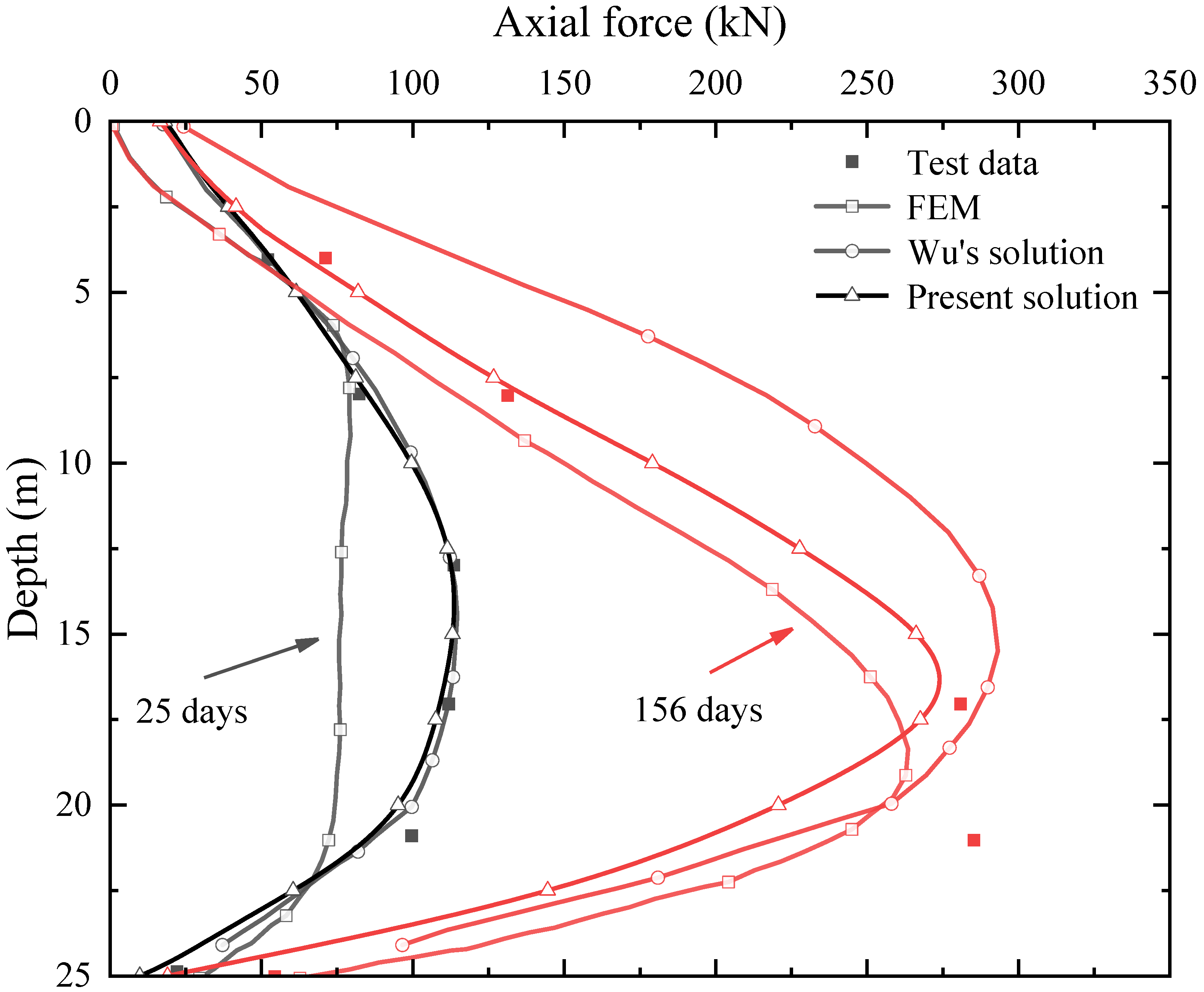
4.1. Case Histories: Yang [31]

To validate the proposed method in this paper, its predicted results were compared with the field test results and the FEM results reported by Yang [31]. There is no surcharge load on the test site and no load was applied to the pile top, only considering the influence of the self-weight of the fill soil, while ignoring the weight of the original soil. The soil profile and pile physical parameters are shown in

Table 1. Physical parameters of the soils surrounding the trial pile.

Soil	$\mathbf{h}\left(\mathbf{m}\right)$	${\gamma }^{\mathbf{\prime }}\left(\mathbf{k}\mathbf{N}/{\mathbf{m}}^3\right)$	${\mathbf{E}}_{\mathbf{s}}\left(\mathbf{k}\mathbf{P}\mathbf{a}\right)$	${\mathbf{k}}_{\mathbf{v}}\left({10}^{-10}\mathbf{m}/\mathbf{s}\right)$	${\mathbf{k}}_{\mathbf{i}}\left(\mathbf{k}\mathbf{P}\mathbf{a}/\mathbf{m}\right)$	${\mathbf{k}}_{\mathbf{b}}\left(\mathbf{k}\mathbf{N}/\mathbf{m}\right)$
fill soil	4.4	7.385	11,477	100	2207	–
original soil	45	9.527	34,364	3.48	6608	37,762

and

Table 2. Trial pile parameters.

$\mathbf{r}\left(\mathbf{m}\right)$	$\mathbf{L}\left(\mathbf{m}\right)$	$\mathbf{E}\left(\mathbf{G}\mathbf{P}\mathbf{a}\right)$
0.25	40	36

, respectively.

The comparison results are shown in Figure 5. Generally, the skin friction and axial force calculation results are in good agreement with the measured data. Due to changes in the soil parameters, the skin friction at the interface of the double-layer foundation exhibits a discontinuity phenomenon. With increasing depth, the NSF above the neutral plane changes significantly, and below the neutral plane, the PSF changes nonlinearly. Based on the field test data, Yang [31] established a numerical model to simulate the distribution of NSF, as shown in Figure 5. Compared to the predictions from the FEM, the proposed analytical solution showed better agreement with field test data, validating its reliability for predicting NSF in artificial islands influenced by soil consolidation.

By comparing the two sets of data, it can be seen that with the increasing consolidation time, the position of the neutral plane decreases, and the maximum NSF and axial force of the pile both increase. The calculated value of the lower part of the pile is slightly larger than the measured value, which is because the theoretical assumption assumes that the soil permeability and compression coefficient remain constant, while in actual engineering, these two parameters will change during the consolidation settlement process, resulting in calculated settlement values larger than actual values, thereby causing the calculated values of the skin friction and axial force larger than the measured values. At 41 days of consolidation, skin friction nears zero due to larger upper soil settlement and unconsolidated lower soil under filling soil’s self-weight. With equal pile and soil displacement at 35–40 m depth, skin friction becomes zero, and axial force on the pile remains small.

4.2. Case Histories: Indraratna et al. [32]

Indraratna et al. [32] conducted field tests in layered soils to investigate the development of NSF and surface settlement after embankment construction. Following pile installation, 2 m of the pile length remained above ground, and a 2 m high embankment was built within 3 days. Long-term monitoring of surface settlement and pile axial force was carried out for 265 days. The soil profile and pile physical parameters are shown in

Table 3. Soil parameters around the pile.

Soil	$\mathbf{h}\left(\mathbf{m}\right)$	${\gamma }^{\mathbf{\prime }}\left(\mathbf{k}\mathbf{N}/{\mathbf{m}}^3\right)$	${\mathbf{E}}_{\mathbf{s}}\left(\mathbf{k}\mathbf{P}\mathbf{a}\right)$	${\mathbf{k}}_{\mathbf{v}}\left({10}^{-9}\mathbf{m}/\mathbf{s}\right)$	${\mathbf{k}}_{\mathbf{i}}\left(\mathbf{k}\mathbf{P}\mathbf{a}/\mathbf{m}\right)$	${\mathbf{k}}_{\mathbf{b}}\left(\mathbf{k}\mathbf{N}/\mathbf{m}\right)$
fill soil	2	7	15,000	7.82	2885	–
original soil	40	7.7	22,000	1.17	4231	24,176

and

Table 4. Pile dimensions.

$\mathbf{r}\left(\mathbf{m}\right)$	$\mathbf{L}\left(\mathbf{m}\right)$	$\mathbf{E}\left(\mathbf{G}\mathbf{P}\mathbf{a}\right)$
0.2	27	30

, respectively.

The predicted results were compared with field test data by Indraratna et al. [32], FEM results by Liang et al. [7], and Wu et al.’s [22] solution, as shown in Figure 6. After 25 days of soil filling, the present solution’s predictions closely matched the field test data. However, at 156 days, some deviation from the field test data was observed, which might be due to the use of a smaller permeability coefficient in the calculations. Chiou et al. [8] suggested that actual drainage conditions could be three-dimensional, and the in situ soil was non-homogeneous, fitting the field test data using a permeability coefficient 10 times larger than the measured parameters. Wu et al. [22] did not account for the elastic region near the neutral point when the soil surrounding the pile was in a plastic state, resulting in significant discrepancies between the predictions and field test data after 156 days of soil filling. In contrast, the present solution considered this stage, leading to a better fit with the field test data. Overall, the proposed analytical method demonstrates its ability to provide satisfactory predictions of skin friction and axial force, while offering better computational efficiency and convergence compared to FEM.

5. Parametric Study

The response of a pile–soil system in artificial islands is influenced by various factors, such as the installation time of the pile foundation, consolidation time, surcharge load, pile head load, and soil parameters (soil compression modulus, permeability, drainage boundary). However, practical geotechnical engineers are more interested in studying the influence of controllable parameters that can effectively eliminate or alleviate the NSF on the deep foundation. For this reason, this section presents the influence of three controllable parameters, namely, the installation time of the pile, the surcharge load applied at the ground, and the pile head load. In the parameter analysis process of this section, the soil and pile parameters used are presented in Table 1 and Table 2.

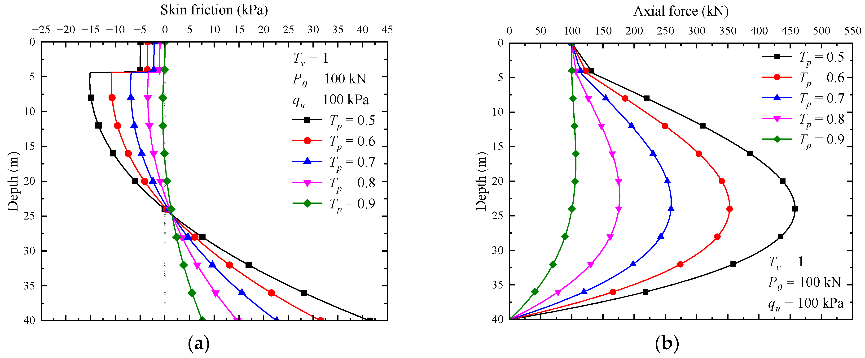
5.1. Case 1: Influence of the Pile Installation Time

Installing pile foundations at a certain interval after filling can effectively alleviate NSF. However, it also extends the construction period. Therefore, in practical engineering, it is necessary to find a balance between effectively reducing NSF generated by soil consolidation and ensuring that the construction period is not too long.

In this case study, the influence of pile installation time is investigated, as shown in Figure 7. To disregard the effects of fill thickness and permeability coefficient on consolidation, the dimensionless time factors ${\mathrm{T}}_{\mathrm{p}}={\mathrm{c}}_{\mathrm{v}1}{\mathrm{t}}_{\mathrm{p}}/{\mathrm{H}}^2$ and ${\mathrm{T}}_{\mathrm{v}}={\mathrm{c}}_{\mathrm{v}1}\mathrm{t}/{\mathrm{H}}^2$ are employed to represent the pile installation time and soil consolidation time, respectively.

As shown in Figure 7a,b, given a constant consolidation time ${\mathrm{T}}_{\mathrm{v}}$, the maximum NSF along the pile and maximum axial force both decrease as ${\mathrm{T}}_{\mathrm{p}}$ increases. Consequently, the position of the neutral plane gradually ascends, and its sensitivity to ${\mathrm{T}}_{\mathrm{p}}$ becomes increasingly significant.

Although the NSF developed along the pile remains significant when ${\mathrm{T}}_{\mathrm{p}}$ = 0.5, which corresponds to 50% of the complete consolidation time (${\mathrm{T}}_{\mathrm{v}}$), it becomes negligible when ${\mathrm{T}}_{\mathrm{p}}$ = 0.9, or 90% of ${\mathrm{T}}_{\mathrm{v}}$. Therefore, it is unnecessary to install piles only after complete soil consolidation, as ${\mathrm{T}}_{\mathrm{p}}$ = 90% ${\mathrm{T}}_{\mathrm{v}}$ is already sufficient to eliminate most of the NSF.

The above analysis primarily discusses the final state of NSF after the complete consolidation of the fill and the original soil. Next, the influence of ${\mathrm{T}}_{\mathrm{v}}$ on NSF is investigated. To make a comparison, two pile installation times, ${\mathrm{T}}_{\mathrm{p}}$ = 0.001 and ${\mathrm{T}}_{\mathrm{p}}$ = 0.5, are selected. As shown in Figure 8a,b and Figure 9a,b, when the pile is installed immediately after the filling (${\mathrm{T}}_{\mathrm{p}}$ = 0.001), the soil consolidation has a significant impact on skin friction. The skin friction along the pile increases sharply with depth as time progresses. However, when the pile is installed after a period of soil consolidation (${\mathrm{T}}_{\mathrm{p}}$ = 0.5), the changes in skin friction are relatively minor. Comparing the skin friction in these two states, it can be concluded that NSF significantly increases when the pile is installed immediately after the fill compared to when it is installed after a period of soil consolidation.

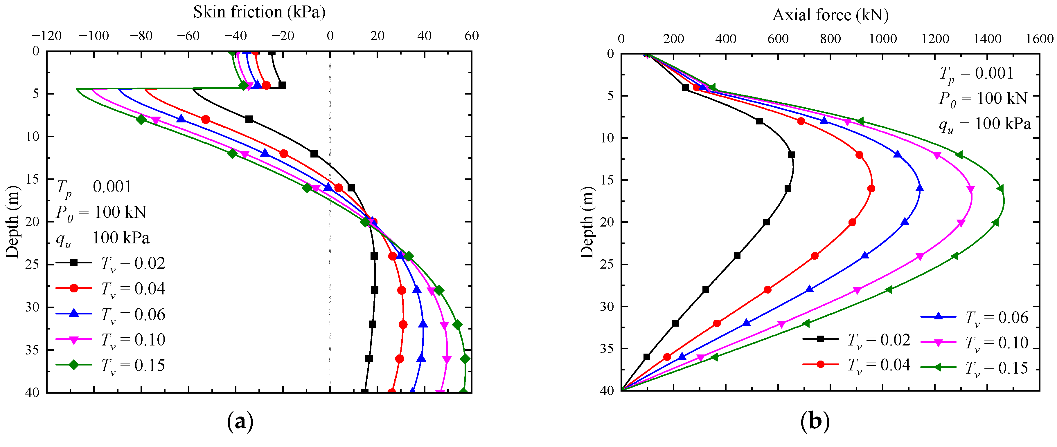
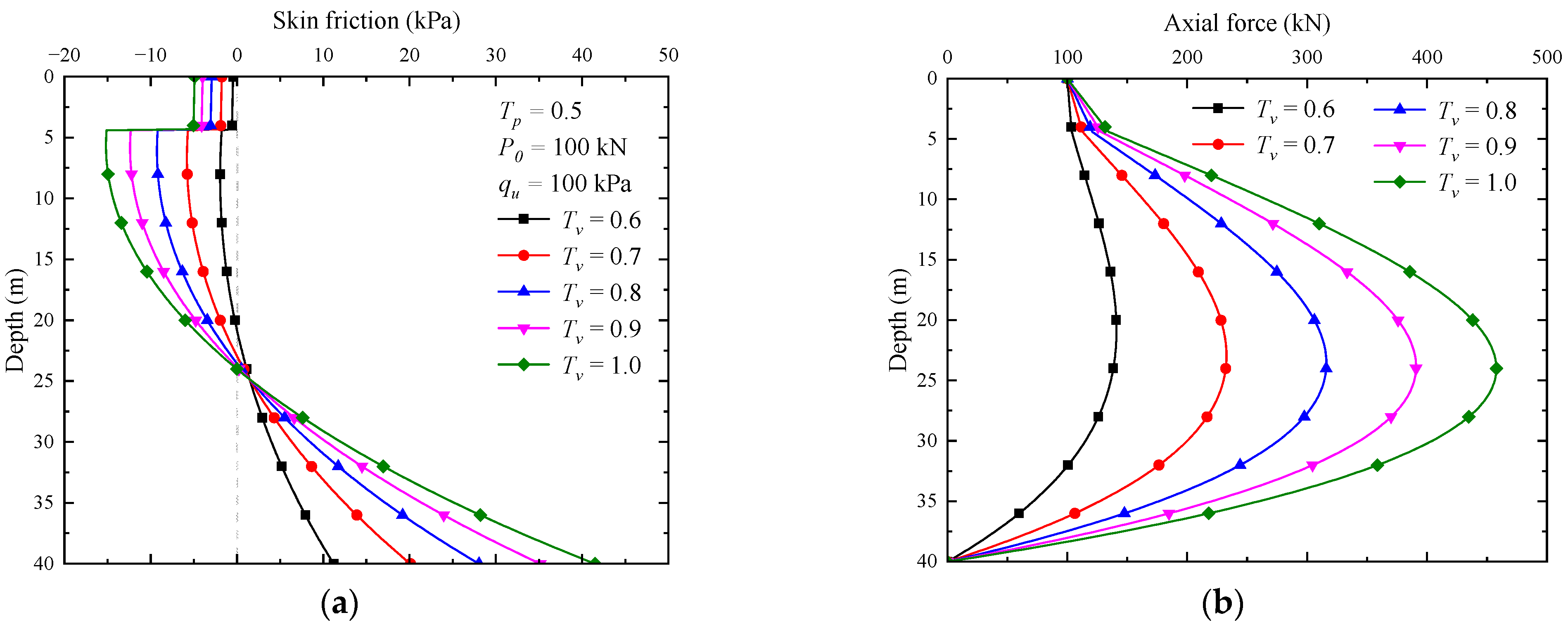
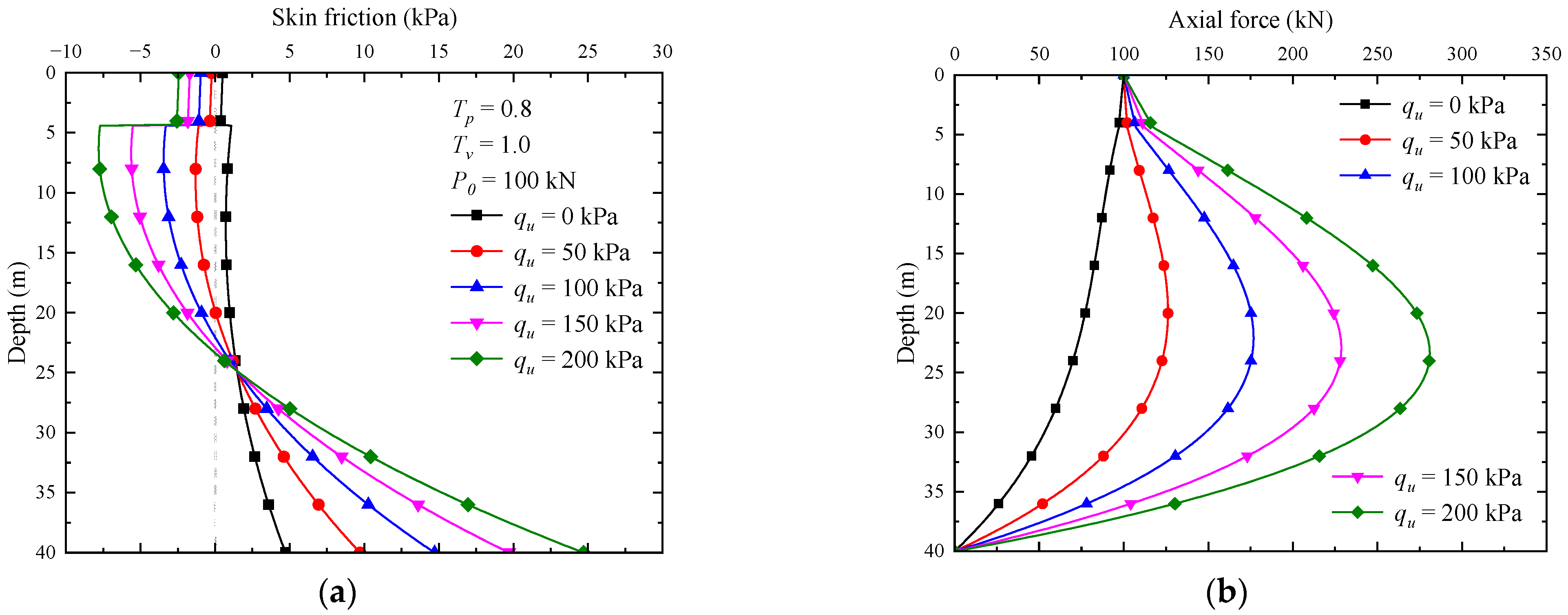
5.2. Case 2: Influence of Surcharge Load

In this case study, the influence of the surcharge load on the distribution of NSF was investigated by installing the pile foundation when the soil was essentially fully consolidated (${\mathrm{T}}_{\mathrm{p}}$ = 0.8) and applying a pile head load of ${\mathrm{P}}_0$ = 100 kN. As shown in Figure 10a, with the increase in the surcharge load, the settlement of the soil caused by consolidation increases, leading to an increase in NSF on the upper part of the pile and the PSF on the lower part of the pile, which will inevitably lead to an increase in the pile axial force, as shown in Figure 10b. The position of the neutral plane will move downward as the surcharge load increases.

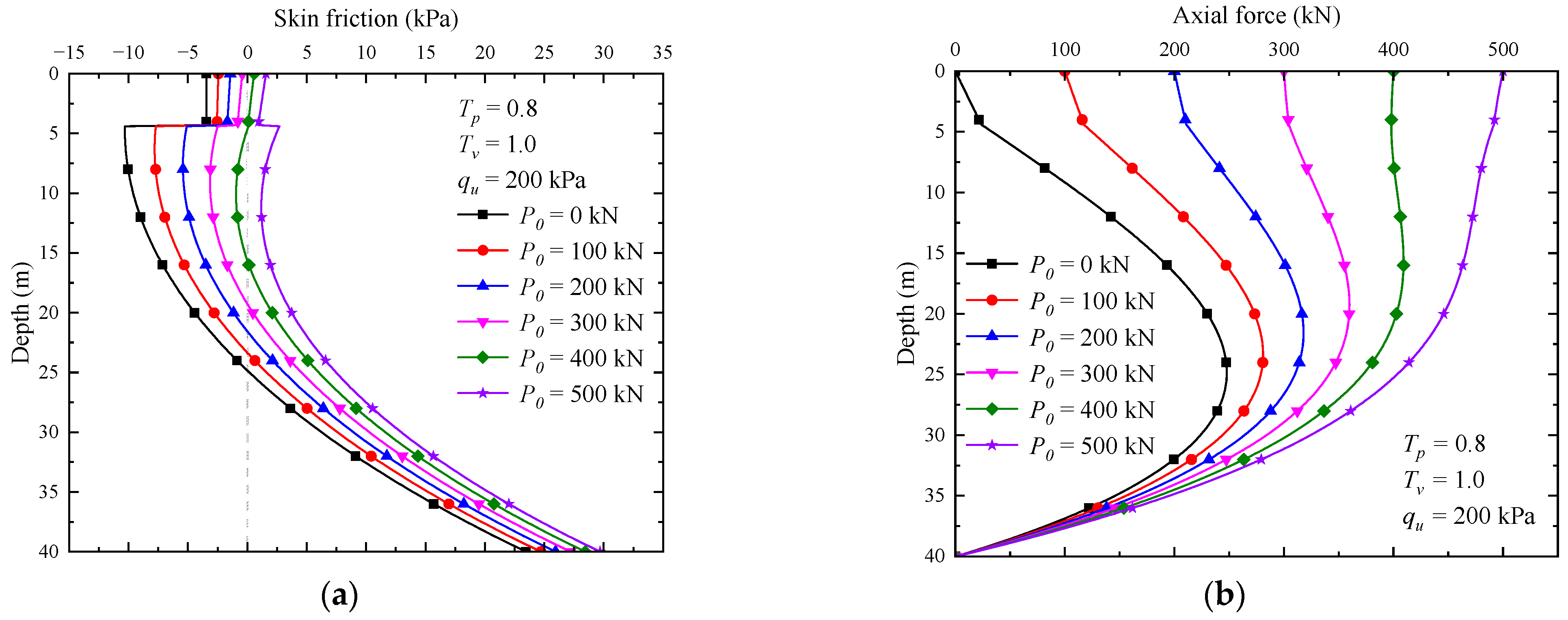
5.3. Case 3: Influence of Pile Head Load

In this case study, the influence of the pile head load on the distribution of NSF was investigated by installing the pile foundation when the soil was essentially fully consolidated (${\mathrm{T}}_{\mathrm{p}}$ = 0.8) and with a value of surcharge load ${\mathrm{q}}_{\mathrm{u}}$ = 200 kPa. The changes in skin friction and axial force with different pile head loads are shown in Figure 11. As the pile head load increases, the NSF gradually decreases, and the location of the neutral plane moves upwards. When the pile head load is sufficiently large, no NSF will be generated. Increasing the pile head load can effectively reduce the influence of soil consolidation on the pile foundation.

In order to fully account for the influence of surcharge load and pile head load on the NSF, the effect of varying pile head loads on the neutral plane position in the pile foundation was calculated for surcharge loads of 200 kPa, 300 kPa, and 400 kPa, respectively. As shown in Figure 12, with the increase in the pile head load, the neutral plane position moves upward, while the influence of the pile head load gradually weakens with the increase in the surcharge load.

6. Conclusions

In this paper, a pile–soil interaction model that incorporates the self-weight consolidation of fill soil to investigate the development of NSF in offshore wind power pile foundations on artificial islands is developed. Analytical solutions for the skin friction and axial force of the pile with respect to time and depth are derived, and the results are in good agreement with the data collected from field tests, FEMs, and other solutions. The above research found that:

(1)

Compared to existing methods, considering the elastic state of the soil near the neutral plane during the plastic stage of pile–soil interaction analysis provides a better prediction of the distribution of NSF under vertical loads considering consolidation;

(2)

Installing pile foundations immediately after soil filling results in NSF several times greater than that of installing piles after a period of consolidation. To balance the reduction of NSF and the shortening of construction time, pile installation can be carried out when ${\mathrm{T}}_{\mathrm{p}}$ = 90% ${\mathrm{T}}_{\mathrm{v}}$;

(3)

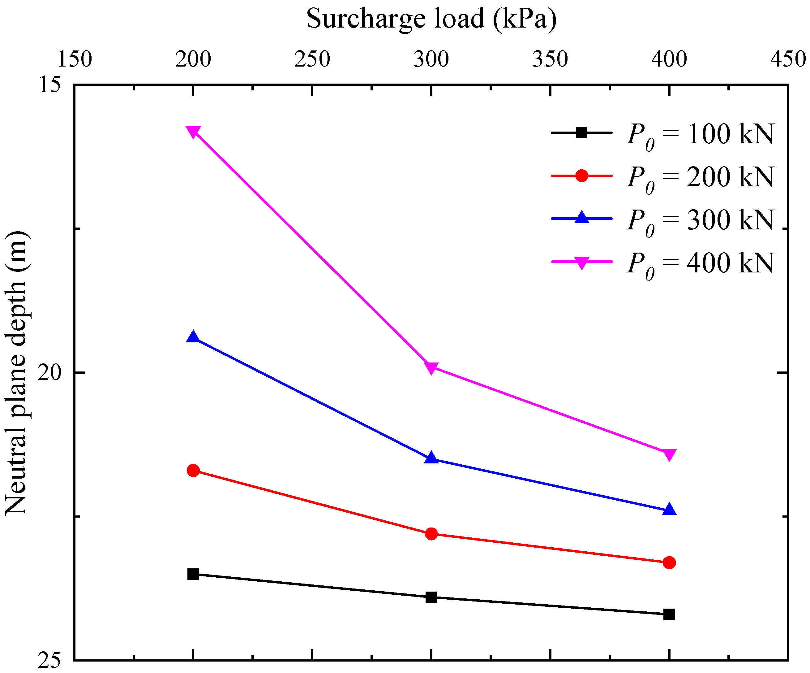
As the surcharge load increases, the increase in NSF inevitably leads to an increase in axial force on the pile, and the position of the neutral plane moves downward. Increasing the pile head load can reduce NSF and raise the neutral plane. This measure effectively mitigates the impact of soil consolidation on pile foundations. However, as the surcharge load increases, the influence of the pile top load gradually diminishes.

References

1. Soares-Ramos, E.P.; de Oliveira-Assis, L.; Sarrias-Mena, R.; Fernández-Ramírez, L.M. Current status and future trends of offshore wind power in Europe. Energy 2020, 202, 117787. [Google Scholar] [CrossRef]
2. Hallak, T.S.; Guedes Soares, C.; Sainz, O.; Hernández, S.; Arévalo, A. Hydrodynamic Analysis of the WIND-Bos Spar Floating Offshore Wind Turbine. J. Mar. Sci. Eng. 2022, 10, 1824. [Google Scholar] [CrossRef]
3. Pérez-Collazo, C.; Greaves, D.; Iglesias, G. A review of combined wave and offshore wind energy. Renew. Sustain. Energy Rev. 2015, 42, 141–153. [Google Scholar] [CrossRef]
4. Salo, O.; Syri, S. What economic support is needed for Arctic offshore wind power? Renew. Sustain. Energy Rev. 2014, 31, 343–352. [Google Scholar] [CrossRef]
5. Jansen, M.; Duffy, C.; Green, T.C.; Staffell, I. Island in the Sea: The prospects and impacts of an offshore wind power hub in the North Sea. Adv. Appl. Energy 2022, 6, 100090. [Google Scholar] [CrossRef]
6. Lee, C.; Ng, C.; Jeong, S. The effect of negative skin friction on piles and pile groups. In Linear and Non-Linear Numerical Analysis of Foundations; CRC Press: Boca Raton, FL, USA, 2009; pp. 193–242. [Google Scholar]
7. Liang, R.; Yin, Z.-Y.; Yin, J.-H.; Wu, P.-C. Numerical analysis of time-dependent negative skin friction on pile in soft soils. Comput. Geotech. 2023, 155, 105218. [Google Scholar] [CrossRef]
8. Chiou, J.-S.; Wei, W.-T. Numerical investigation of pile-head load effects on the negative skin friction development of a single pile in consolidating ground. Acta Geotech. 2021, 16, 1867–1878. [Google Scholar] [CrossRef]
9. Jeong, S.; Ko, J.; Lee, C.; Kim, J. Response of single piles in marine deposits to negative skin friction from long-term field monitoring. Mar. Georesources Geotechnol. 2014, 32, 239–263. [Google Scholar] [CrossRef]
10. Rituraj, S.S.; Giridhar Rajesh, B. Negative skin friction on piles: State of the art. In Advances in Geo-Science and Geo-Structures: Select Proceedings of GSGS 2020; Springer: Berlin/Heidelberg, Germany, 2022; pp. 323–335. [Google Scholar]
11. Abdrabbo, F.M.; Ali, N.A. Behaviour of single pile in consolidating soil. Alex. Eng. J. 2015, 54, 481–495. [Google Scholar] [CrossRef]
12. Shen, K.; Wang, K.; Yao, J.; Yu, J. Numerical Investigation on Behavior of Compressive Piles in Coastal Tidal Flat with Fill. J. Mar. Sci. Eng. 2022, 10, 1742. [Google Scholar] [CrossRef]
13. Chow, Y.; Lim, C.; Karunaratne, G. Numerical modelling of negative skin friction on pile groups. Comput. Geotech. 1996, 18, 201–224. [Google Scholar] [CrossRef]
14. Wang, J.; Zhou, D.; Zhang, Y.; Cai, W. Vertical impedance of a tapered pile in inhomogeneous saturated soil described by fractional viscoelastic model. Appl. Math. Model. 2019, 75, 88–100. [Google Scholar] [CrossRef]
15. Cheng, H.W.; Cheng, Z.; Jiang, C.; Li, Y. Influences of ultimate frictional resistance at low confining pressure on bearing characteristics of backfill piles. Yantu Gongcheng Xuebao/Chin. J. Geotech. Eng. 2018, 40, 87–90. [Google Scholar]
16. Kim, H.-J.; Mission, J.L.; Park, T.-W.; Dinoy, P.R. Analysis of negative skin-friction on single piles by one-dimensional consolidation model test. Int. J. Civ. Eng. 2018, 16, 1445–1461. [Google Scholar] [CrossRef]
17. Fellenius, B.H. Results from long-term measurement in piles of drag load and downdrag. Can. Geotech. J. 2006, 43, 409–430. [Google Scholar] [CrossRef]
18. Ng, C.W.; Poulos, H.G.; Chan, V.S.; Lam, S.S.; Chan, G.C. Effects of tip location and shielding on piles in consolidating ground. J. Geotech. Geoenviron. Eng. 2008, 134, 1245–1260. [Google Scholar] [CrossRef]
19. Yu, P.; Dong, J.; Liu, H.; Xu, R.; Wang, R.; Xu, M.; Liu, H. Analysis of cyclic shear stress–displacement mechanical properties of silt–steel interface in the Yellow River Delta. J. Mar. Sci. Eng. 2022, 10, 1704. [Google Scholar] [CrossRef]
20. Mindlin, R.D. Force at a point in the interior of a semi-infinite solid. Physics 1936, 7, 195–202. [Google Scholar] [CrossRef]
21. Cao, W.; Chen, Y.; Wolfe, W. New load transfer hyperbolic model for pile-soil interface and negative skin friction on single piles embedded in soft soils. Int. J. Geomech. 2014, 14, 92–100. [Google Scholar] [CrossRef]
22. Wu, W.; Wang, Z.; Zhang, Y.; El Naggar, M.H.; Wu, T.; Wen, M. Semi-analytical solution for negative skin friction development on deep foundations in coastal reclamation areas. Int. J. Mech. Sci. 2023, 241, 107981. [Google Scholar] [CrossRef]
23. Kim, H.J.; Mission, J.L.C. Negative skin friction on piles based on finite strain consolidation theory and the nonlinear load transfer method. KSCE J. Civ. Eng. 2009, 13, 107–115. [Google Scholar] [CrossRef]
24. Liu, Y.; Yang, P.; Xue, S.; Pan, Y. Influence of dredger fill self-consolidation on development of negative skin friction of piles. Arab. J. Geosci. 2020, 13, 725. [Google Scholar] [CrossRef]
25. Terzaghi, K. Erdbaumechanik Auf Bodenphysikalischer Grundlage; F. Deuticke, Leipzig and Wien: Leipzig, Germany, 1925. [Google Scholar]
26. Xie, K.H. Theory of One Dimensional Consolidation of Double-Layered Ground and its Applications. Chin. J. Geotech. Eng. 1994, 16, 24–35. [Google Scholar]
27. Randolph, M.F.; Wroth, C.P. Analysis of deformation of vertically loaded piles. J. Geotech. Eng. Div. 1978, 104, 1465–1488. [Google Scholar] [CrossRef]
28. Wong, K.; Teh, C. Negative skin friction on piles in layered soil deposits. J. Geotech. Eng. 1995, 121, 457–465. [Google Scholar] [CrossRef]
29. Castelli, F.; Maugeri, M. Simplified nonlinear analysis for settlement prediction of pile groups. J. Geotech. Geoenviron. Eng. 2002, 128, 76–84. [Google Scholar] [CrossRef]
30. Fellenius, B.H. Effective stress analysis and set-up for shaft capacity of piles in clay. In From Research to Practice in Geotechnical Engineering; ASCE: Reston, VA, USA, 2008; pp. 384–406. [Google Scholar]
31. Yang, J.J. Bearing Performance and Computational Method of Piles in Hydraulic-Reclamation Area. Master’s Thesis, Shanghai Jiaotong University, Shanghai, China, 2014. [Google Scholar]
32. Indraratna, B.; Balasubramaniam, A.; Phamvan, P.; Wong, Y. Development of negative skin friction on driven piles in soft Bangkok clay. Can. Geotech. J. 1992, 29, 393–404. [Google Scholar] [CrossRef]
Figure 1. Pile–soil interaction model of double-layer foundation.
Jmse 11 01071 g001
Figure 2. Load transfer model of (a) skin friction; (b) pile tip resistance.
Jmse 11 01071 g002
Figure 3. Pile–soil interaction model at different stages.
Jmse 11 01071 g003
Figure 4. One-dimensional consolidation model of (a) the double-layer foundation; (b) surcharge load versus time curve.
Jmse 11 01071 g004
Figure 5. Comparisons of the present solution, field test data, and FEM results on distribution of (a) skin friction; (b) axial force.
Jmse 11 01071 g005
Figure 6. Comparisons of predicted results, field test data, and FEM results on distribution of axial force.
Jmse 11 01071 g006
Figure 7. Influences of pile installation time T p on distribution of (a) skin friction; (b) axial force.
Jmse 11 01071 g007
Figure 8. Influences of soil consolidation time T v for pile installation time T p = 0.001 on distribution of (a) skin friction; (b) axial force.
Jmse 11 01071 g008
Figure 9. Influences of soil consolidation time T v for pile installation time T p = 0.5 on distribution of (a) skin friction; (b) axial force.
Jmse 11 01071 g009
Figure 10. Influences of surcharge load q u on distribution of (a) skin friction; (b) axial force.
Jmse 11 01071 g010
Figure 11. Influences of pile head load P 0 on distribution of (a) skin friction; (b) axial force.
Jmse 11 01071 g011
Figure 12. Depth of the neutral plane.
Jmse 11 01071 g012