Article

Output Feedback Tracking Control with Collision Avoidance for Dynamic Positioning Vessel under Input Constraint

1
College of Intelligent Systems Science and Engineering, Harbin Engineering University, Harbin 150001, China
2
China Classification Society, Beijing 100007, China
*
Author to whom correspondence should be addressed.
J. Mar. Sci. Eng. 2023, 11(4), 811; https://doi.org/10.3390/jmse11040811
Submission received: 10 March 2023 / Revised: 30 March 2023 / Accepted: 5 April 2023 / Published: 11 April 2023
(This article belongs to the Special Issue Motion Control and Path Planning of Marine Vehicles)

Abstract

:
This dissertation presents a fresh control strategy for dynamic positioning vessels exposed to model uncertainty, various external disturbances, and input constraint. The vessel is supposed to work in a particular situation surrounding a lighthouse or a submerged reef, where collision avoidance must be prevented. The control strategy involves making the vessel navigate under the action of modified artificial potential functions (MAPFs) along a smooth trajectory. To achieve this goal, we put forward a collision-avoidance control strategy, which consists of the backstepping technique, an extended state observer (ESO), and an active dynamic positioning control technique. The MAPFs, together with a strategy, are applied to realize collision avoidance. To address the input constraint problem, an auxiliary dynamic system (ADS) is constructed. Entire related signals of the control system could converge to a small neighboring zone of the equilibrium state via Lyapunov deduction. Simulation outcomes verify the effectiveness of the presented control strategy.

1. Introduction

As an increasingly widely used tool for exploring and exploiting marine resources, the motion control strategy of dynamic positioning vessels has attracted increasing attention [1,2,3,4]. The study and investigation on the control method of dynamic positioning vessels have been sufficient. However, due to model uncertainty and the effects of environmental disturbances, undertaking research remains challenging [5,6,7]. To deal with this challenge, several control methods have been proposed for the tracking control of dynamic positioning vessels. In general, control schemes used for compensating the model uncertainty and disturbances can be classified as passive and active approaches. The active approaches exploit the estimation of the model uncertainty and disturbances to compensate for these effects [8], while the passive approaches rely on the robustness property of the designed controller [9,10,11]. To reduce the ship roll motion in waves, a self-tuning proportional integral derivative (PID) controller is used to adjust optimal stabilizer fin angles in [12]. However, the controller has poor performance to deal with the high magnitude of the disturbance values. In order to increase the performance, fuzzy logic systems and intelligent control techniques have been proposed in [13,14]. The fuzzy logic systems depend on a good human understanding of the dynamical behavior of the system. Model predictive control is employed to ensure optimal system performance [15], and the method algorithm requires a large number of account operations and resources. To solve this problem and enhance robustness property, sliding mode control is proposed for the tracking control of dynamic positioning vessels [16]. To reduce the effects of uncertainty and disturbances, an active approach is designed based on observers. In order to estimate uncertainty and disturbances, the disturbance observer is proposed for the tracking control of vessels [17]; the key features of disturbance observer are based on velocity measurements. The position and heading of vessels can be acquired by using GPS and electronic compass, although it is difficult to obtain their velocities. To avoid using velocity measurements, a nonlinear extended state observer (ESO) is employed for dynamic positioning vessel in [18].
Besides model uncertainty and disturbances, another challenge to tracking control for dynamic positioning vessel is input constraint. Due to physical limitations, the actuator outputs are constantly bounded or constrained [19]. Input constraint may degrade the system performance and lead to an imbalance [20]. To deal with this challenge, a Gaussian error function is used to approximate input saturation in [21]. The hyperbolic tangent function is used to handle the input saturation in [22], and a trajectory tracking control law is designed based on the hyperbolic tangent function. However, the hyperbolic tangent function and Gaussian error function limit system performance, even if the control inputs are not saturated. To avoid this, an anti-windup compensator is incorporated into controller design to solve trajectory tracking of dynamic positioning vessel with input saturation in [23]. To solve the input saturation in trajectory tracking control of vessels, an auxiliary dynamic system (ADS) is applied to controller design in [24]. Ref. [25] introduces an auxiliary control to solve the formation control of autonomous underwater vehicles with input saturation.
However, few papers take the problem of collision-avoidance control into account. In the view of engineering practice, it is inevitable for unmanned vessels to encounter fixed or moving obstacles such as lighthouses and submerged reefs. Collision avoidance is crucial to navigation safety. The existing achievements often use a path-planning algorithm to solve the collision-avoidance problem [26,27,28,29]. The method depends on an optimization algorithm, which is complex and takes a long time to obtain a feasible solution, so it is not conducive to lowering the construction cost of dynamic positioning vessels. In order to address this problem, some scholars design the control system of unmanned vessels with collision avoidance [30,31]. However, input saturation is neglected in the controller-design process, and the performance of the actuator has a great impact on collision-avoidance ability. Therefore, input constraint also needs to be considered when proposing the collision-avoidance control algorithm.
Motivated by the above research background, this paper investigates the trajectory tracking control of surface vessels subject to input saturation, uncertainty, and environmental disturbances. Even more significantly, both static obstacles and unknown non-cooperative ships are taken into consideration. Inspired by the works in [30], an improved output feedback controller is proposed. Firstly, an ESO is used to estimate the velocity, model uncertainty, and disturbances. To avoid collisions with obstacle and unknown non-cooperative ships, modified artificial potential functions (MAPFs) are incorporated into the controller-design process. In particular, MAPFs can render the vessel bypass obstacle and unknown non-cooperative ships smoothly, which greatly reduces the actuator performance requirements. An ADS is introduced to solve the input saturation. Then, an output feedback controller is designed based on the ESO, the MAPFs, and the ADS. Finally, the stability of closed-loop system is proved. Simulations demonstrate the proposed control strategy.
Three salient features of this paper are summarized as follows. First, MAPFs are designed to solve the problem of automatic collision avoidance system for dynamic positioning vessels. Second, both obstacle and unknown non-cooperative ships are considered in the controller-design process. The embedded processor of the vessels carries out reading computations using only the position and yaw, and the transmission loads are saved. Third, the designed strategy can achieve collision avoidance, even if the control inputs are saturated.
Compared with the existing related results, the novelty of this paper is summarized as follows. First, compared with the control strategy [20,21,22,23], this paper designs a strategy to achieve collision avoidance between a vessel and an obstacle. Second, unlike the existing control approaches [30,31], input saturation is considered in the controller-design process; the proposed controller has become more attractive in practice engineering. Third, compared with the collision-avoidance algorithm proposed in [18], a non-cooperative ship is also considered.
The other sections are organized as follows. The problem is formulated in Section 2. Section 3 provides a collision-avoidance strategy, Section 4 presents an observer design, and Section 5 presents a controller design and stability analysis. Simulation outcomes are described in Section 6. Conclusions are given in Section 7.

2. Problem Formulation

The kinematic (position and orientation) and dynamic (linear velocity and angular velocity) models of dynamic positioning vessel are [32]
η ˙ = R ( ψ ) ν
M ν ˙ + C ν + D ν = τ + d ,
where  η = [ x , y , ψ ] T , x, and y are vertical and horizontal coordinates in the earth-fixed reference frame, respectively.  ψ  is the yaw angle in the earth-fixed reference frame.  ν = [ u , v , r ] T  denotes the velocity vector containing linear velocity u, v and the angular velocity r M R 3 × 3  denotes the inertia matrix including added mass, which is positive definite, invertible, and constant.  C R 3 × 3  represents a skew-symmetric matrix of Coriolis and centripetal term.  D R 3 × 3  denotes the damping matrix, which is positive definite.  τ = [ τ u , τ v , τ r ] T  is the input signal.  d = [ d 1 , d 2 , d 3 ] T  are the environmental disturbances.  R ( ψ )  is the rotation matrix and given by
R ( ψ ) = c o s ( ψ ) s i n ( ψ ) 0 s i n ( ψ ) c o s ( ψ ) 0 0 0 1 .
In practical application, due to the limited engine power, the input signals are limited by maximum force and moment. The input limitation is given:
τ = τ max τ c > τ max τ c τ min τ c τ max τ min τ c < τ min
where  τ max  and  τ min R 3  are the maximum and minimum control force and moment, respectively. The mismatch function is defined as  = τ c τ τ c = [ τ u c , τ v c , τ r c ] T τ u c τ v c  and  τ r c  are control force and moment calculated by the proposed controller, respectively. The saturated input signal can be attained by  τ = τ c .

3. Collision Avoidance Strategy

The collision-avoidance ability of the control system plays an important role in ship-collision avoidance and ensuring the safety of ship navigation, and artificial potential functions are used for achieving collision avoidance [33,34]. Here, the MAPFs are designed; they consist of a repulsion function, and they do not work when the vessel is sufficiently far away from obstacle and other ship. The MAPFs repel the vessel when the vessel approaches the obstacle and the other ship, which keeps a safe distance from the obstacle and the other ship. The obstacle is modeled as a circle-shaped object [35], and the MAPFs are given as follows:
p o = 1 2 α o ( 1 p v 1 R ¯ o ) 2 , if p v R ¯ o 0 , o t h e r w i s e
where  p v = p p o  is the distance between the vessel and the obstacle,  p = [ x , y ] T  is the position of the vessel,  p o = [ x o , y o ] T  is the center of the obstacle, and  α o  is a positive constant.  R ¯ o = max { R o , R u } R o  is the collision avoidance range with respect to the obstacle, and  R u  is the collision avoidance range with respect to the vessel.
To avoid collision with an obstacle, the MAPFs are introduced to the control objective. Additionally, the control objective is given as follows:
lim t + η η d η o < c 1
where  η d  is the desired trajectory,  η o = [ p o , p o , 0 ] T .
Hypothesis 1.
η d  and its derivative  η ˙ d  are bounded.
Remark 1.
The MAPFs do not work when the vessel is sufficiently far away from obstacle. This means that  η o = [ 0 , 0 , 0 ] T  if  p v > R ¯ o , and the control objective is a trajectory tracking task. The MAPFs work and repel the vessel when it approaches the obstacle. The design of  η o  ensures that the MAPFs can render the vessel bypass obstacle smoothly, which leads to conservative input signals.

4. Observer Design

In this section, we develop a nonlinear observer to estimate the unknown term containing environmental disturbances d, the damping matrix D, and the Coriolis and centripetal term C; the model of USV can be rewritten as
η ˙ = R ( ψ ) ν
ν ˙ = M 1 τ + ζ ,
where  ζ = M 1 ( C ν D ν + d ) .
Hypothesis 2.
There is a positive constant  ζ *  such that  ζ ˙ ζ * .
Inspired by [36], an ESO is given to provide the estimations of model uncertainties and disturbances, which is shown as:
η ^ ˙ = K o 1 ( η ^ η ) + R ( ψ ) ν ^ ,
ν ^ ˙ = K o 2 R T ( ψ ) ( η ^ η ) + ζ ^ + M 1 τ ,
ζ ^ ˙ = K o 3 R T ( ψ ) ( η ^ η )
where  η ^ = [ x ^ , y ^ , ψ ^ ] T R 3 ν ^ = [ u ^ , v ^ , r ^ ] T R 3 ζ ^ = [ ζ ^ 1 , ζ ^ 2 , ζ ^ 3 ] T R 3 x ^ y ^ ψ ^ u ^ v ^ r ^ ζ ^ 1 ζ ^ 2 ζ ^ 3  are the estimates of x, y ψ , u, v, r ζ 1 ζ 2  and  ζ 3 K o 1 R 3 × 3 K o 2 R 3 × 3 , and  K o 3 R 3 × 3  are gain matrices.
From (5)–(9), the error dynamics of the ESO are given as
η ˜ ˙ = K o 1 η ˜ + R ( ψ ) ν ˜ , ν ˜ ˙ = K o 2 R T ( ψ ) η ˜ + ζ ˜ , ζ ˜ ˙ = K o 3 R T ( ψ ) η ˜ ζ ˙ ,
where  η ˜ = η ^ η ν ˜ = ν ^ ν  and  ζ ˜ = ζ ^ ζ  are estimation errors.
The observer error dynamics (10) can be rewritten as
X ˙ = A X + B ϕ
η ˜ = C o X ,
where  X = [ η ˜ T , ν ˜ T , ζ ˜ T ] T R 9 × 1 ,
A = K o 1 R ( ψ ) 0 3 K o 2 R T ( ψ ) 0 3 I 3 K o 3 R T ( ψ ) 0 3 0 3 ,
B = 0 3 0 3 I 3 ,
C o i = I 3 0 3 0 3 ,
ϕ = ζ ˙ 0 3  is a  3 × 3  dimensional zero matrix.  I 3  is a  3 × 3  dimensional identity matrix.
According to Hypothesis 2, we can devise a hypothesis that  ϕ ϕ ¯  and  ϕ ¯  is a positive constant.
A nonlinear term  J ( ψ )  makes it difficult to conduct the stability analysis of the ESO. To solve the difficulty, a transformation  χ = T X  with  T = d i a g { J T ( ψ ) I 3 , I 3 }  is introduced, thus
χ ˙ = ( A 0 + r S T ) χ + B ϕ ,
where  S T = d i a g { S 1 , 0 3 , 0 3 } ,
S 1 = 0 1 0 1 0 0 0 0 0 ,
A 0 = K o 1 I 3 0 3 K o 2 0 3 I 3 K o 3 0 3 0 3 .
Lemma 1.
The error of the ESO X is bounded, if there are symmetric definite positive matrices  Q , P R 9 × 9  such that
A 0 T P + P A 0 + P B B T P + Q + r ¯ ( S T T P + P S T ) 0 ,
A 0 T P + P A 0 + P B B T P + Q r ¯ ( S T T P + P S T ) 0 ,
r ¯ R  is the upper bound of r.
Chose a Lyapunov function as follows:
V o = 1 2 χ T P χ .
We can obtain that  V ˙ o = 1 2 ( χ T P χ ˙ + χ ˙ T P χ ) .  Form (16), we can obtain that
V ˙ o = 1 2 ( χ T P ( ( A 0 + r S T ) χ + B ϕ ) ) + 1 2 ( ( A 0 + r S T ) χ + B ϕ ) T P χ
By using  ( ( A 0 + r S T ) χ ) T P χ = χ T ( A 0 T p + r S T T P ) χ  and  ( B ϕ ) T P χ = χ T P B ϕ , differentiating  V o  with respect to time is given:
V o = 1 2 χ T ( P A 0 + A 0 T P + r P S T + r S T T P ) χ + χ T P B ϕ 1 2 χ T ( P A 0 + A 0 T P + r P S T + r S T T P + P B B T P ) χ + 1 2 ϕ T ϕ c o 1 V o + c o 2 ,
where  c o 1 = λ min ( Q ) λ max ( P ) c o 2 = 1 2 ϕ ¯ 2 . Since  c o 2  is symmetric definite positive, the state  χ i  is bounded. Using  T 1 = 1  and  X = T 1 χ , the estimation error signal X is bounded.

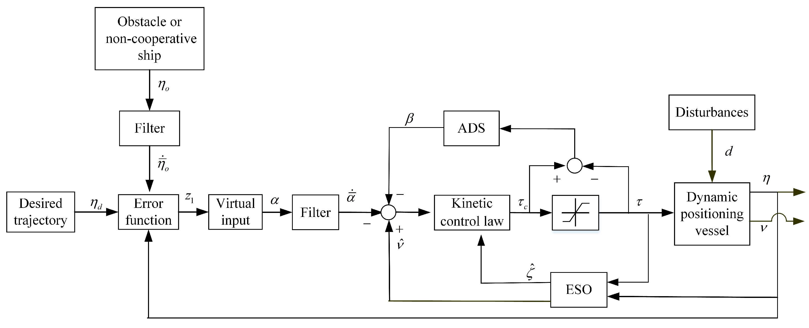
5. Controller Design

In order to clearly describe the process of controller design, the diagram of the proposed output feedback controller is given in Figure 1. The designed ESO provides estimations of velocities, model uncertainty, and disturbances by using position of the vessel. A filter is used to give the velocity estimations of obstacle or non-cooperative ship. An ADS is designed based on the mismatch function  = τ c τ . The proposed kinetic control law is designed by using the ADS and the ESO.
An output feedback controller design for vessel with collision avoidance is presented step by step.
Step 1: A modified error function based on the information of desired trajectory and obstacle is defined as
z 1 = η η d η o .
Along with the kinematics (5), the time derivative of (24) is given as
z ˙ 1 = R ( ψ ) ν η ˙ d η ˙ o .
Choosing  α  as a virtual input, the kinematic control law  α  is proposed as
α = R T ( ψ ) ( η ˙ d + η ¯ ˙ o K 1 z 1 ) ,
where  K 1 R 3 × 3  is a diagonal matrix,  η ˙ d  is known time derivative of  η d η ¯ ˙ o  is the signal originated from the filter, and  l o η ¯ ˙ o + η ¯ o = η o l o  is a positive constant.
Remark 2.
The virtual input (26) is a virtual velocity signal. If  z 1  and  η ¯ ˙ o [ 0 , 0 , 0 ] T α R T ( ψ ) η ˙ d , which is the desired velocity in the hull coordinate system. If  z 1 [ 0 , 0 , 0 ] T  and  η ¯ ˙ o [ 0 , 0 , 0 ] T α R T ( ψ ) ( η ˙ d + η ¯ ˙ o ) , the velocity of the vessel converges to the vector piled up by the desired velocity and the velocity of obstacle. The term  K 1 z 1  ensures the convergence of the signal α, the therms  η ˙ d + η ¯ ˙ o  give equilibrium points of the control system, and the  R T ( ψ )  is the transform matrix between the earth-fixed reference frame and the hull coordinate system.
Remark 3.
Narrow channels and coastal waters form regions with heavy maritime traffic. Small sea vehicles do not have navigational aids such as VHF radio or AIS [37]. Users are unable to gain the velocity information. We refer to these actors as non-cooperative ships. Non-cooperative ships need to be taken into account in controller design. To estimate the velocity information of non-cooperative ships, a filter is introduced to the process of controller design. Errors are caused when the velocity estimation is used. Errors are bounded due to position-bounded  η o . This shows that enough safety distance between dynamic positioning vessels and non-cooperative ships or obstacles is necessary.
Step 2: In this step, a dynamic controller at the kinetic level is developed. Define the second error vector as
z 2 = ν ^ α ¯ β ,
where  β  is signal of ADS; it is designed to solve input saturation.  α ¯  is introduced to avoid the calculation of the time derivative of  α ; a first-order filter is used instead of the time derivative of  α l α ¯ ˙ + α ¯ = α  with time constant  l > 0 . The update law of  β  is given as
β ˙ = K 2 β M 1
where  K 2 R 3 × 3  is a diagonal matrix.
The time derivative of  z 2  is derived as
z ˙ 2 = K o 2 R T ( ψ ) η ˜ + ζ ^ + M 1 ( τ c ) α ¯ ˙ β ˙ .
To stabilize  z 2 , a kinetic control law is designed as
τ c = M ( K 3 z 2 ζ ^ + α ¯ ˙ + K 2 β R T ( ψ ) z 1 ) ,
where  K 3 R 3 × 3  is a diagonal matrix.
Lemma 2.
Consider the system consisting of the dynamic positioning vessel dynamics (1) and (2); the kinetic control law (30); the observer (7), (8), and (9); and the ADS (28) with input saturation, environmental disturbances, and model uncertainty. If Hypotheses 1–2 are satisfied, the proposed output feedback-control scheme guarantees that all of the signals in the closed-loop system are bounded.
Proof. 
Choose a Lyapunov function candidate as follows:
V 1 = 1 2 z 1 T z 1 .
Using (25), the time derivative of  V 1  is given
V ˙ 1 = z 1 T [ R ( ψ ) ν η ˙ d η ˙ o ] .
By applying (27) to (32), the time derivative of  V 1  is rewritten as
V ˙ 1 = z 1 T [ R ( ψ ) ( z 2 + α + β + α ˜ ν ˜ ) η ˙ d η ˙ o ] .
Substituting (26) into (33), the time derivative of  V 1  can be rewritten as
V ˙ 1 = z 1 T K 1 z 1 + z 1 T [ R ( ψ ) ( z 2 + β + α ˜ ν ˜ ) ] + Δ v ,
where  Δ v  is a positive constant containing estimate error of the velocity information of non-cooperative ships.
Define a another Lyapunov function
V 2 = V 1 + 1 2 z 2 T z 2 .
Form (8), (27), and (34), the time derivative of  V 2  can be attained
V ˙ 2 = z 1 T K 1 z 1 + z 1 T [ R ( ψ ) ( z 2 + β + α ˜ ν ˜ ) ] + z 2 T [ K o 2 R T ( ψ ) η ˜ + ζ ^ + M 1 ( τ c ) α ¯ ˙ β ˙ ] + Δ v
Using equations (30) and (28),
V ˙ 2 = z 1 T K 1 z 1 + z 1 T [ R ( ψ ) ( β + α ˜ ν ˜ ) ] z 2 T K o 2 R T ( ψ ) η ˜ .
Define the last Lyapunov function
V 3 = V 2 + 1 2 β T β + V o .
Using (28) and (37) yields, the time derivative of  V 3  is given
V ˙ 3 = z 1 T K 1 z 1 z 2 T K 3 z 2 + z 1 T [ R ( ψ ) ( β + α ˜ ν ˜ ) ] z 2 T K o 2 R T ( ψ ) η ˜ β T K 2 β β M 1 + Δ v + V ˙ o .
Using Young’s inequality, the inequalities are given as
z 1 T [ R ( ψ ) ( β + α ˜ ν ˜ ) ] 1 2 ( 3 z 1 T z 1 + β T β + α ˜ T α ˜ + ν ˜ T ν ˜ ) ,
z 2 T K o 2 R T ( ψ ) η ˜ λ min ( K o 2 ) / 2 ( z 2 T z 2 + η ˜ T η ˜ ) ,
β M 1 1 / 2 ( β T β + Δ ) ,
where  Δ = M 1 T M 1 .
Substituting (40)–(42) into (39), the time derivative of  V 3  is rewritten as
V ˙ 3 [ λ min ( K 1 ) 3 / 2 ] z 1 T z 1 [ λ min ( K 3 ) λ min ( K o 2 ) / 2 ] z 2 T z 2 [ λ min ( K 2 ) 1 ] β T β c o 3 V o + c o 4 ,
where  c o 3 = [ λ min ( Q ) max { λ min ( K o 2 ) , 1 } ] / λ max ( P ) c o 4 = c o 2 + α ˜ T α ˜ + Δ / 2 + Δ v .
The inequality (43) becomes
V ˙ 3 c 1 V 3 + c 2 ,
where  c 1 = min { 2 [ λ min ( K 1 ) 3 / 2 ] , 2 [ λ min ( K 3 ) λ min ( K o 2 ) / 2 ] , 2 [ λ min ( K 2 ) 1 ] , c o 3 } c 2 = c o 4 .
From the definition of  V 3 , it can be concluded that all of the signals in the closed-loop are bounded. □

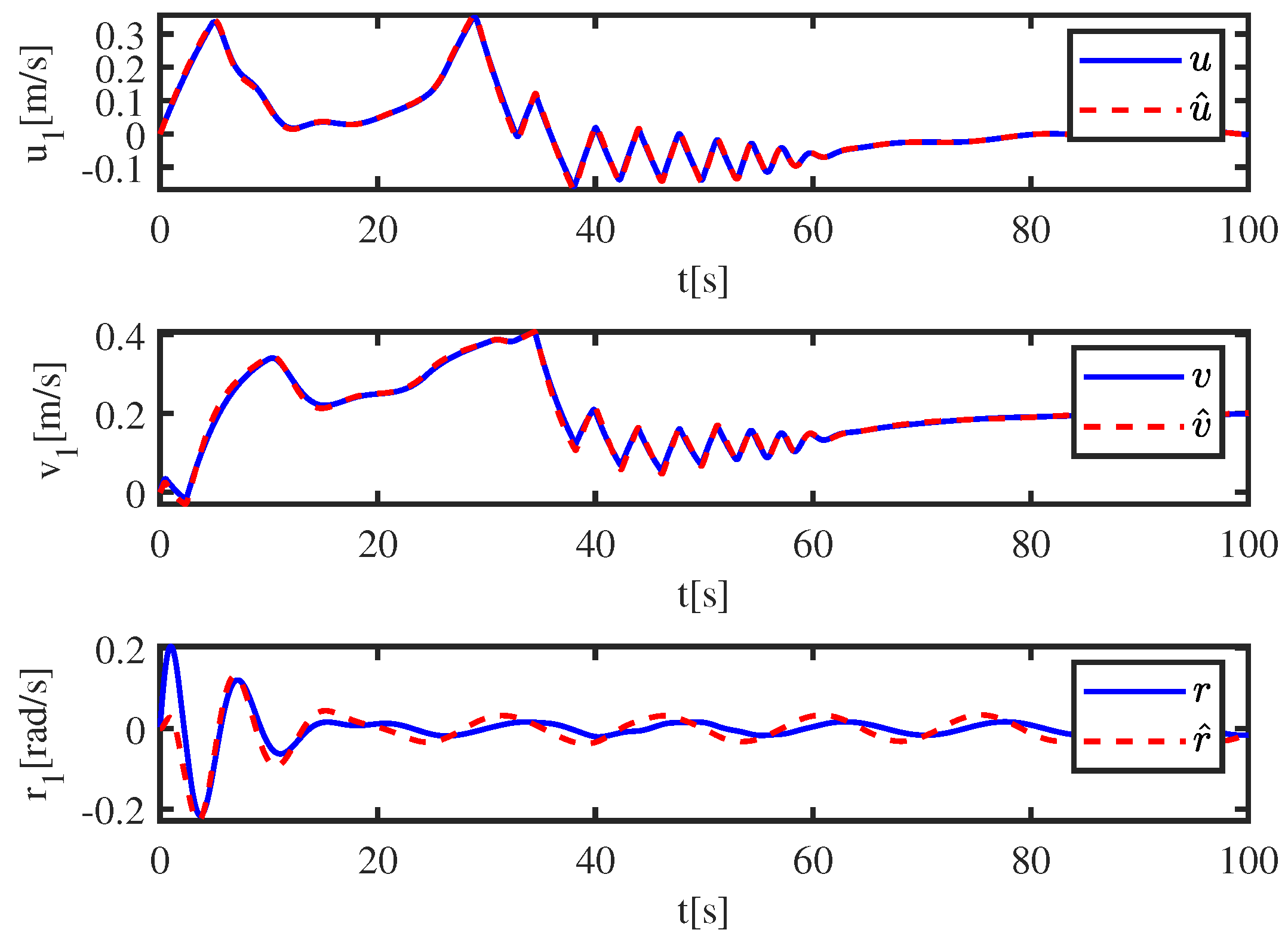
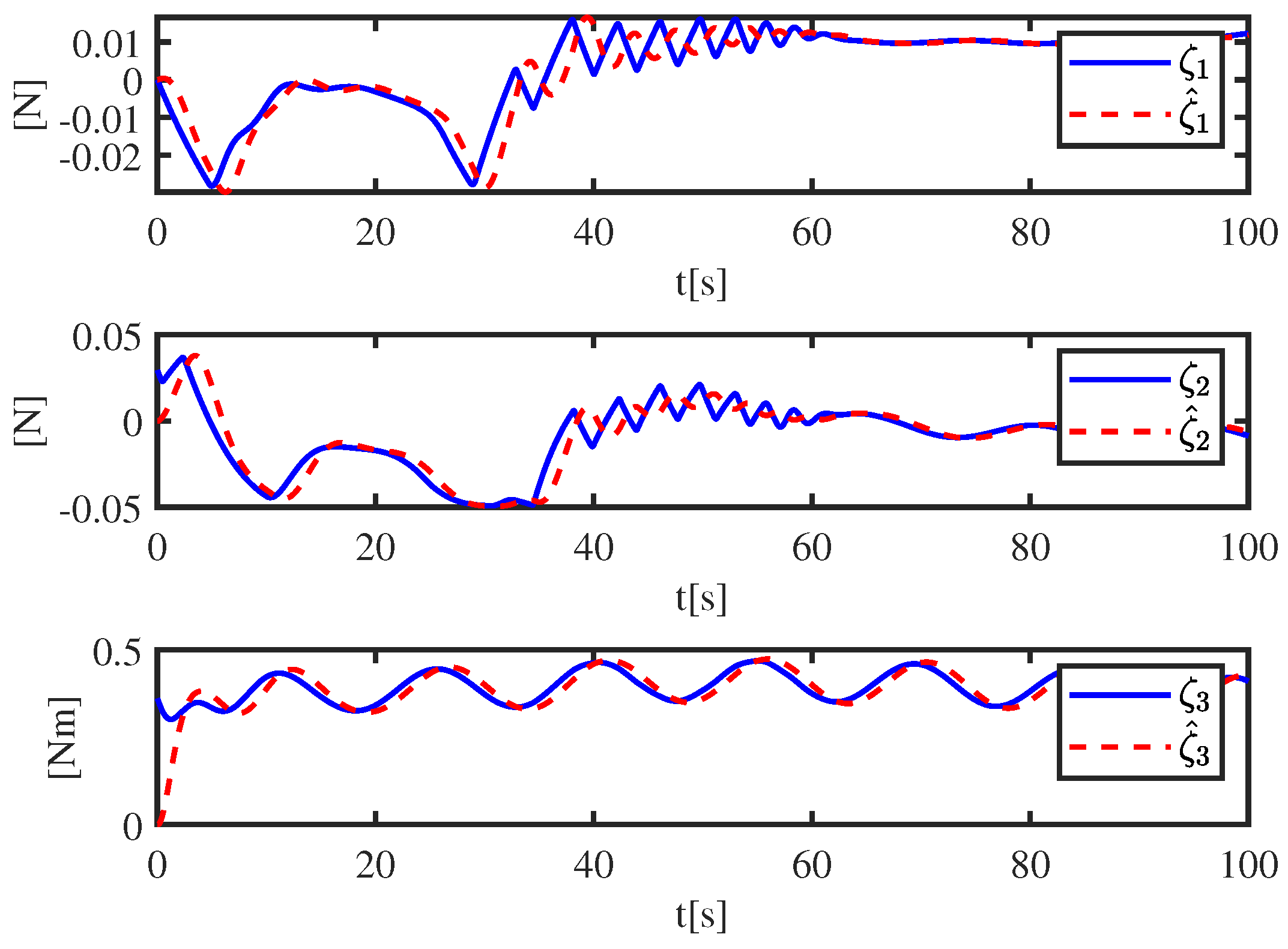
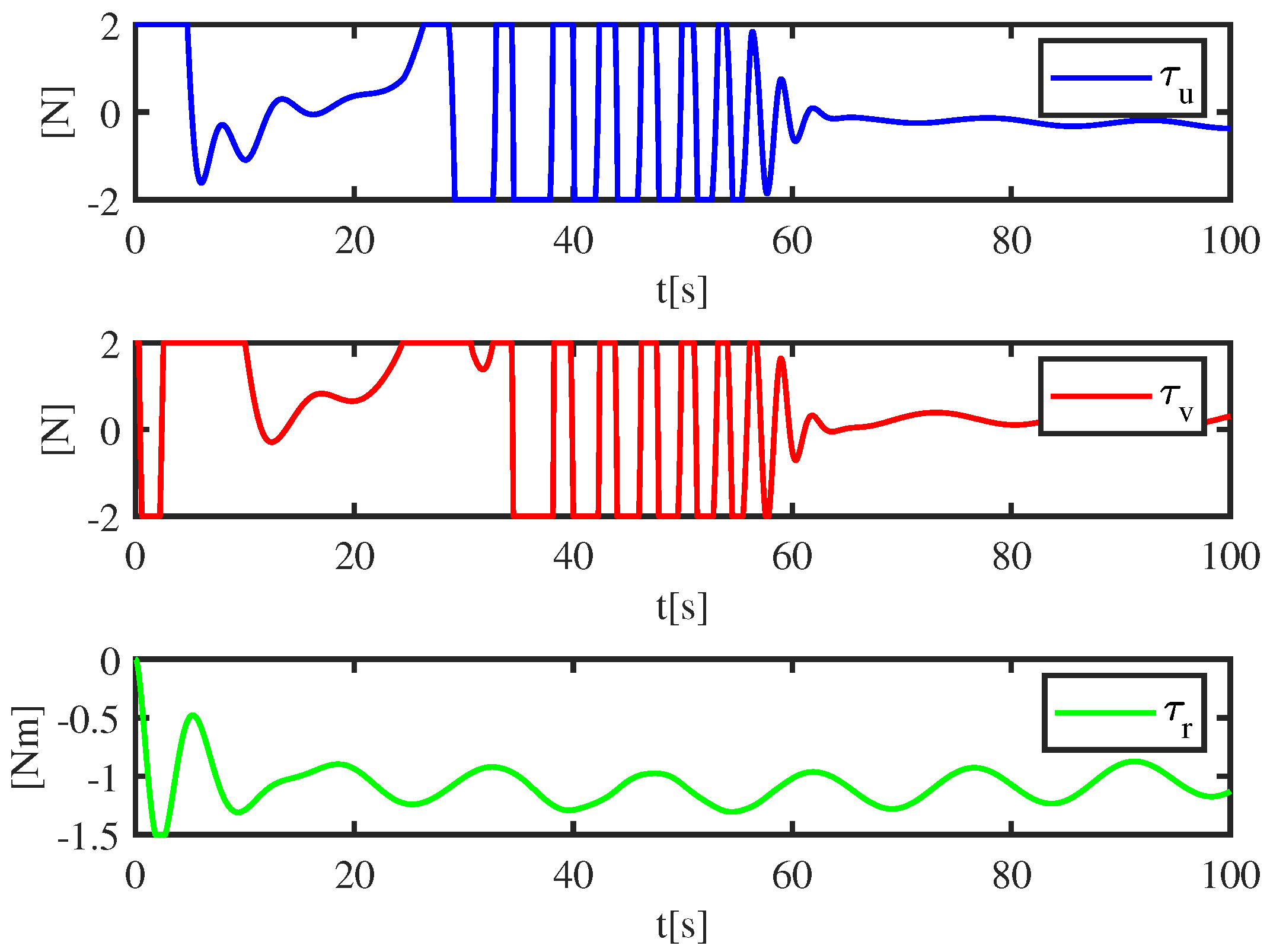
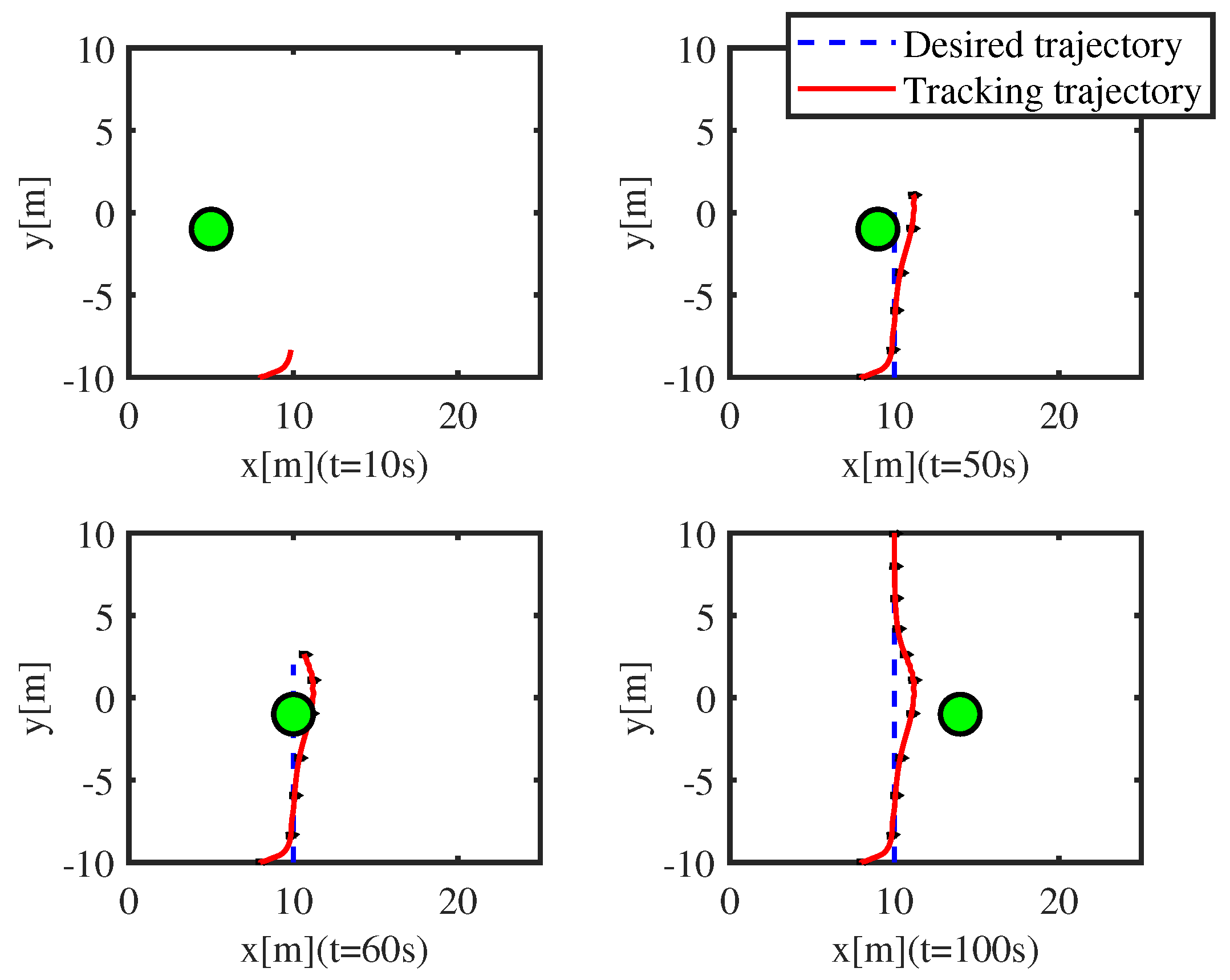
6. Simulation Results

In this section, numerical simulations are designed to show the effectiveness of the proposed controller (PC). The reference signal  η d  is used to generate desired trajectory. In simulations, the model of dynamic positioning ship Cybership II is used [38]. The control forces and moment are constrained as  τ max = [ 2  N, 2 N , 1.5  Nm],  τ min = [ 2  N,  2  N , 1.5  Nm]. Environmental disturbances are modeled as the sum of some sinusoidal signals. The parameters of observer are chosen as  K o 1 = d i a g [ 15 , 15 , 15 ] K o 2 = d i a g [ 15 , 15 , 15 ] K o 3 = d i a g [ 15 , 15 , 15 ] . The design parameters of the controller are  K 1 = d i a g [ 5 , 5 , 5 ] K 2 = d i a g [ 10 , 10 , 10 ] K 3 = d i a g [ 5 , 5 , 5 ] . The avoidance ranges  R ¯ o = 8  m,  α o = 20 .

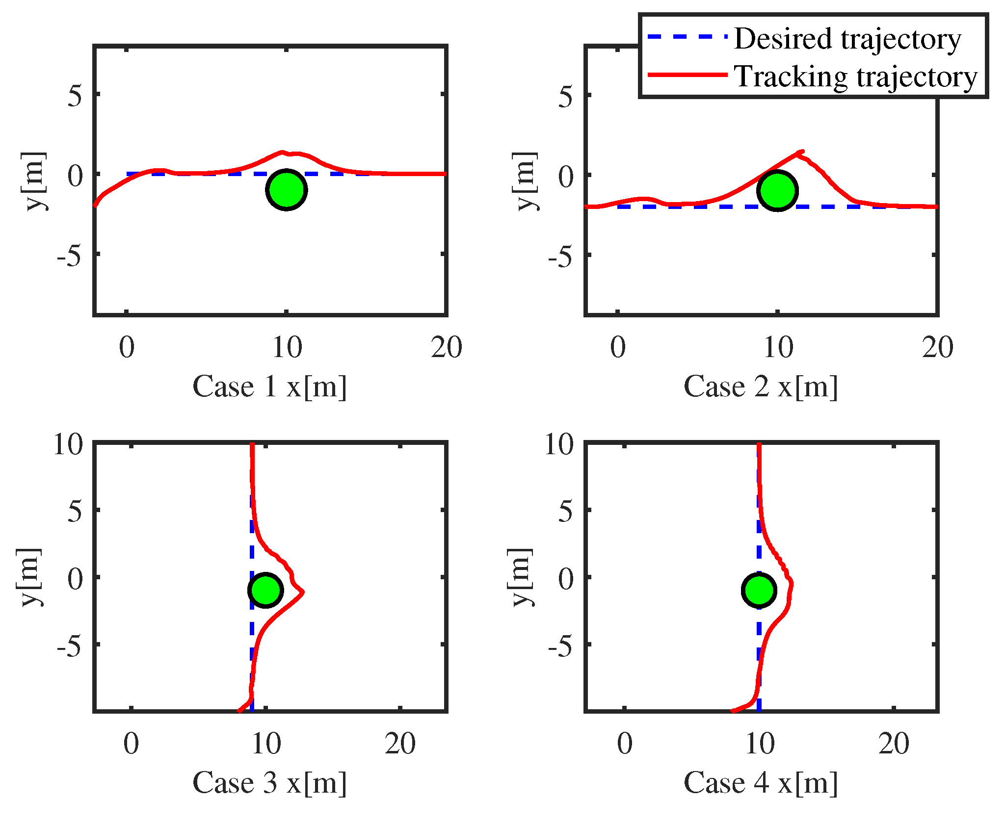
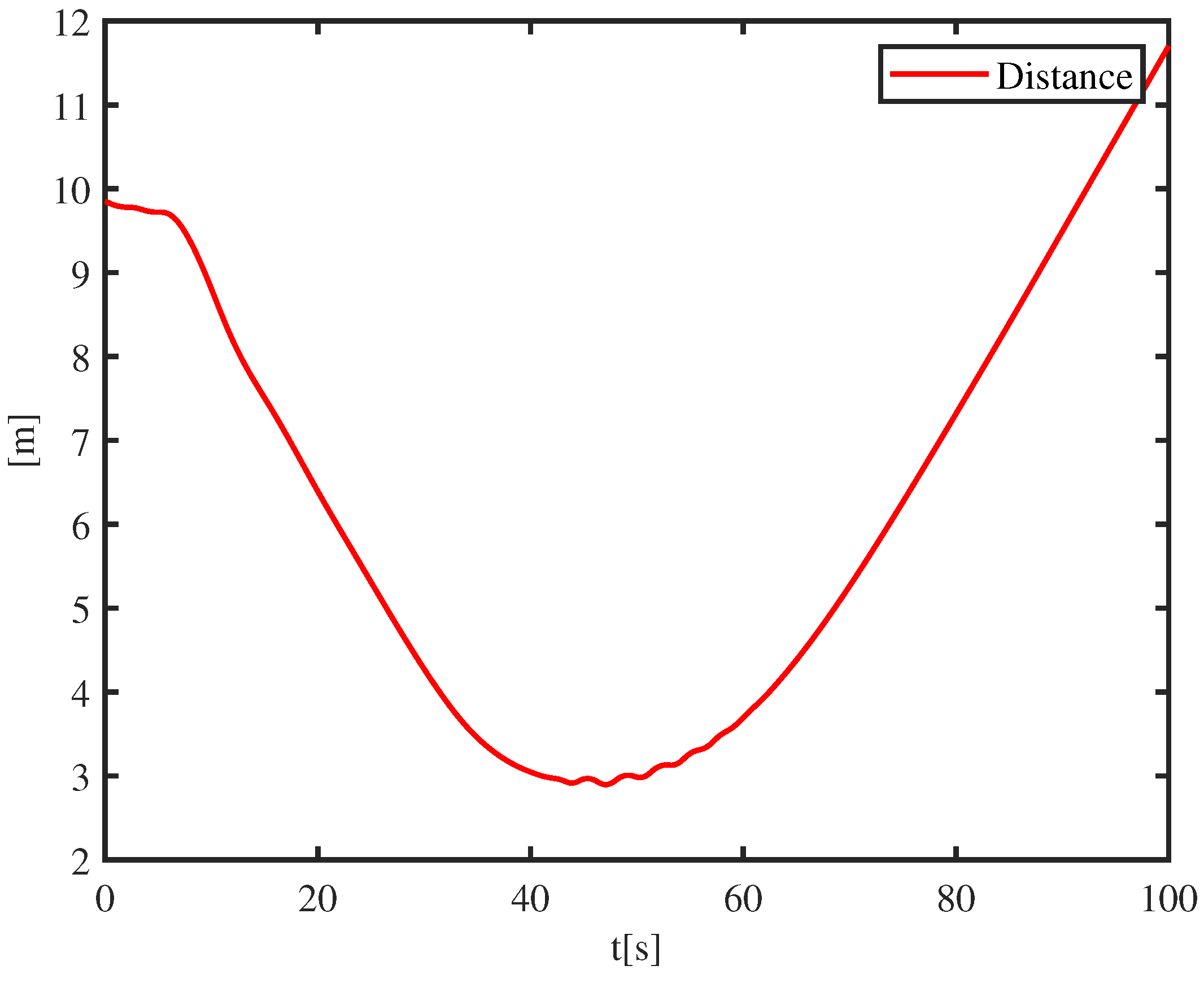
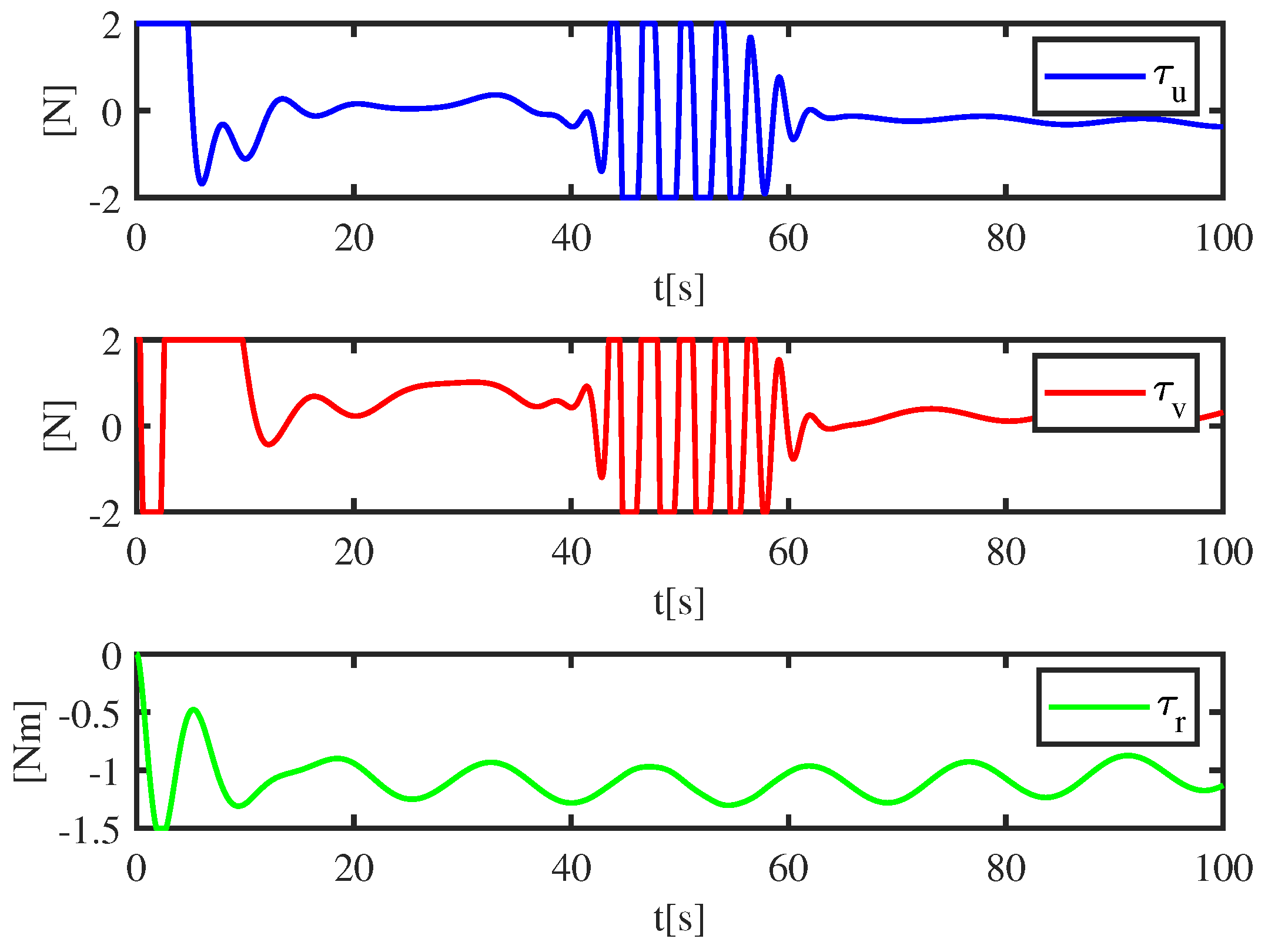
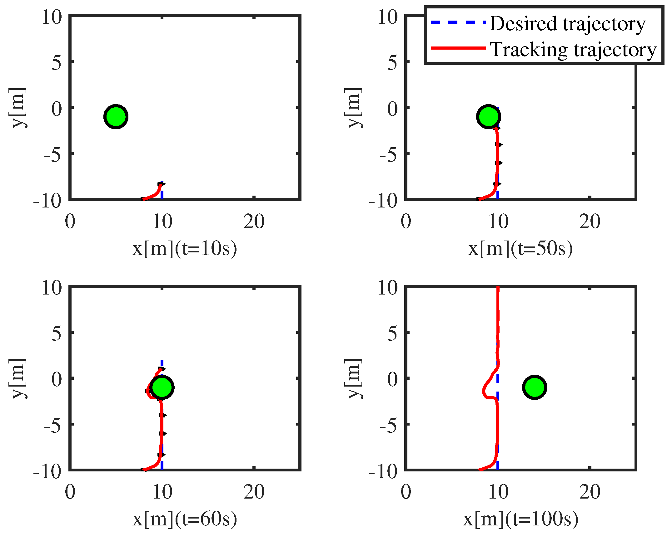
6.1. Trajectory Tracking Control with Obstacle Avoidance

The formation tracking results for case 1, case 2, case 3, and case 4 are shown in Figure 2 and Figure 3. For all cases, the initial postures of desired trajectory are given in  [ 0  m, 0 m, 0 rad ] T . The trajectory is generated by time-varying velocity vector  ν d , and  ν d ( t )  is given in Table 1. The center of the obstacle is presented in Table 1, and the safe collision-avoidance radii is  1.5  m. The initial postures of dynamic positioning vessel  η ( 0 )  are chosen in Table 1.
Figure 2 shows trajectory tracking control under four cases. In all cases, the dynamic positioning vessel overtakes the obstacle on its portside, and it makes a detour around the obstacle. Figure 3 shows the distances between the dynamic positioning vessel and the obstacle. The results show all of the distances are greater than the safe collision-avoidance radii. This explains why there are no safety risks during voyaging: collisions between the dynamic positioning vessel and the obstacle are avoided. To describe the collision-avoidance process, Figure 4 shows the time-varying error function  z 1 T z 1  containing the tracking error  z 1 . In 0 s–25 s, the tracking error  z 1  gradually converges to the neighboring zone of zero, and the MAPFs are ineffective. During 25 s–45 s, the dynamic positioning vessel is moving toward the obstacle, and the MAPFs start to work, which leads to the actual operation deviating from the predetermined trajectory. At 45 s–60 s, the dynamic positioning vessel is moving away from the obstacle, the error function  z 1 T z 1  decreases continuously, and the dynamic positioning vessel gets back on the predetermined trajectory. At 60 s–100 s, the dynamic positioning vessel keeps a safe distance from the obstacle, and the MAPFs do not work.
Figure 5 describes the velocity recovery performance of the observer. At 25 s–60 s, owing to the effect of the MAPFs, the lateral speed and longitudinal speed are changing zigzag. Figure 6 shows that the uncertainty and disturbances can be estimated by the proposed observer, and the estimated initial value is set as zero. Figure 7 shows that the input signals of system are constrained by the input saturation. At 25 s–60 s, to ensure the safety navigation of the dynamic positioning vessel, the MAPFs work and affect the input signals, which generates terrible twitter and saturated input signals.

6.2. Trajectory Tracking Control with Non-Cooperative Ship

To show the effectiveness of the collision-avoidance ability of the PC, a non-cooperative ship is considered in trajectory tracking control. The initial position of non-cooperative ship is set as  [ 4  m,  1  m, 0 rad ] T , and the constant velocity non-cooperative ship is set as  [ 0.1  m/s, 0 m/s, 0 rad/s ] T . Figure 8 shows the trajectory-tracking results. At  t = 10  s, the dynamic positioning vessel tracks the desired signal successfully. The non-cooperative ship comes from port side of the dynamic positioning vessel. At  t = 50  s, the non-cooperative ship takes no actions to avoid collisions, and the dynamic positioning vessel turns to avoid a collision with the non-cooperative ship, which leads to large formation tracking errors. The dynamic positioning vessel overtakes the non-cooperative ship from its starboard. At  t = 60  s, the dynamic positioning vessel keeps a safe distance between the non-cooperative ship, and tracking trajectory gradually converges to the desired trajectory. The non-cooperative ship is moving out from behind the dynamic positioning vessel. At  t = 100  s, the dynamic positioning vessel successfully tracks the desired trajectory again. The dynamic positioning vessel moves away from the non-cooperative ship, and the non-cooperative ship sails on the starboard of the dynamic positioning vessel. Figure 9 demonstrates the distance between the dynamic positioning vessel and the non-cooperative ship. Figure 10 depicts the bounded control force and moment. Under the effect of the ADS, the rapid saturation of the input signals is fast convergence.

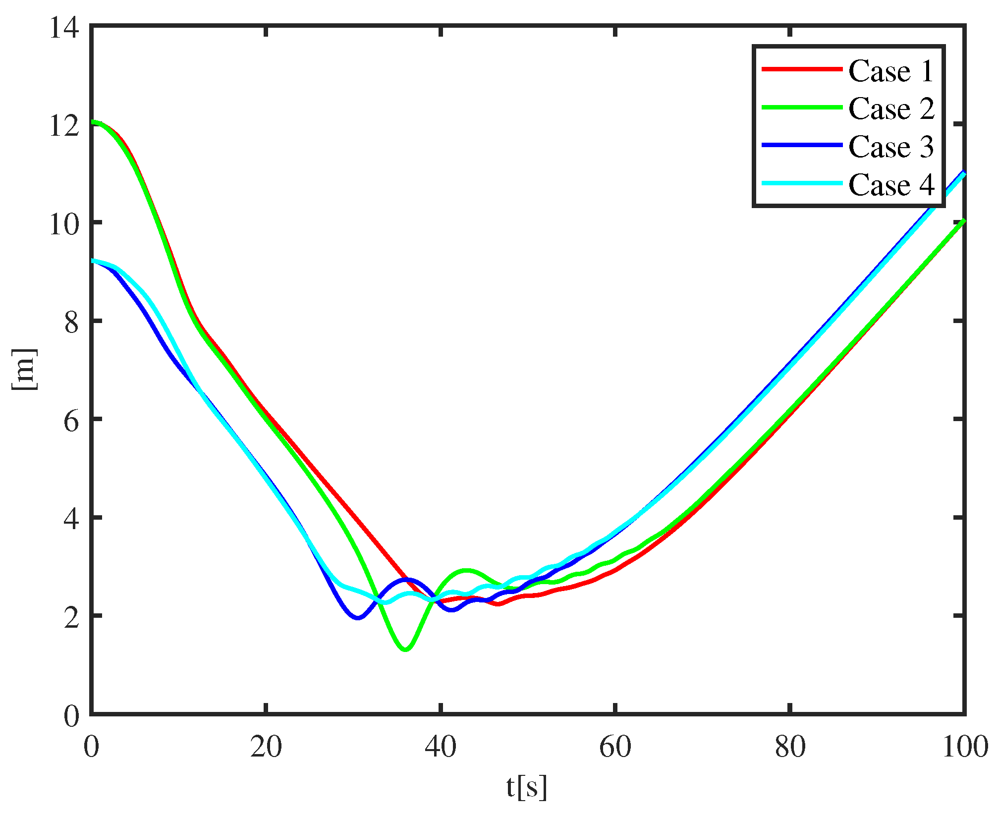
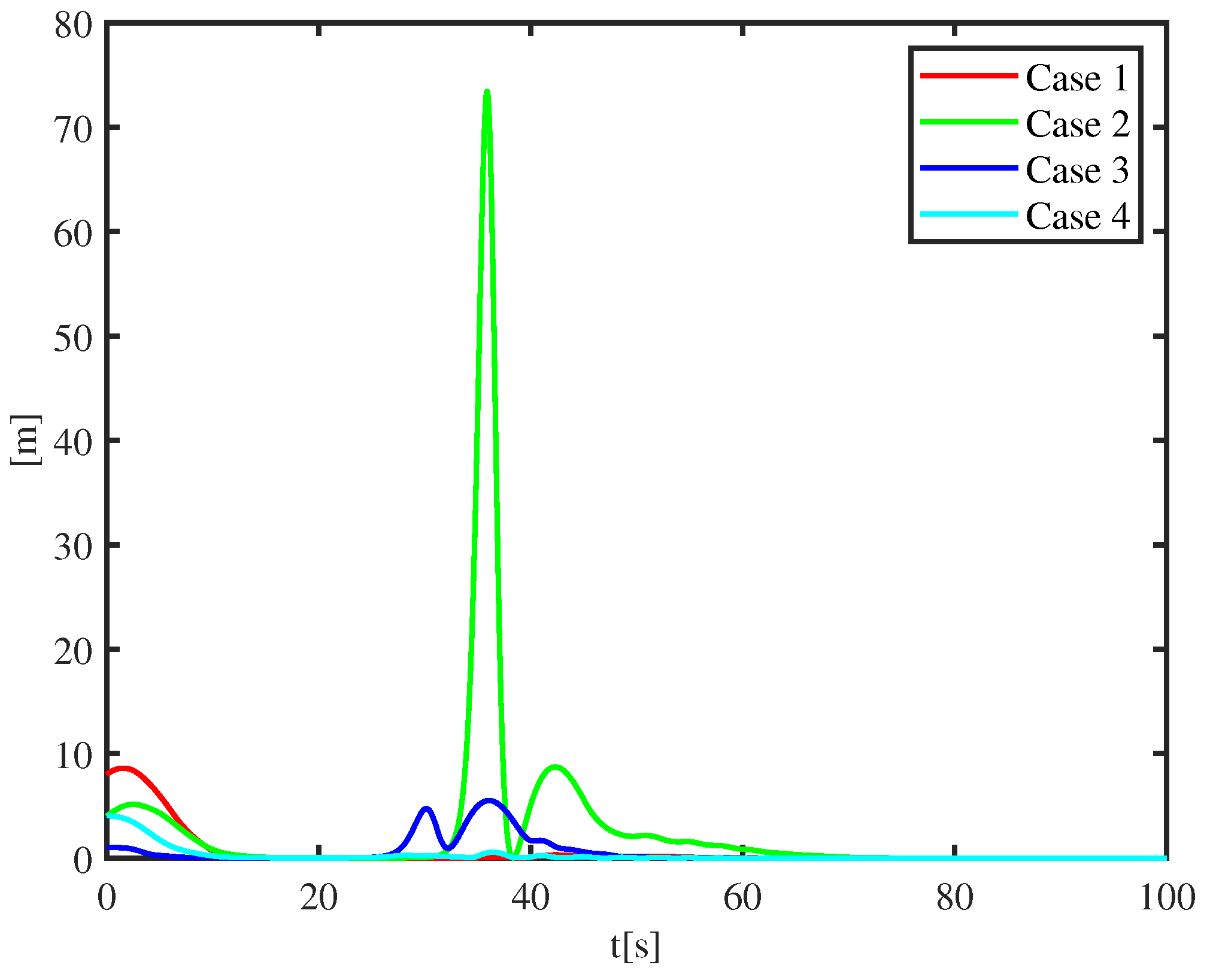
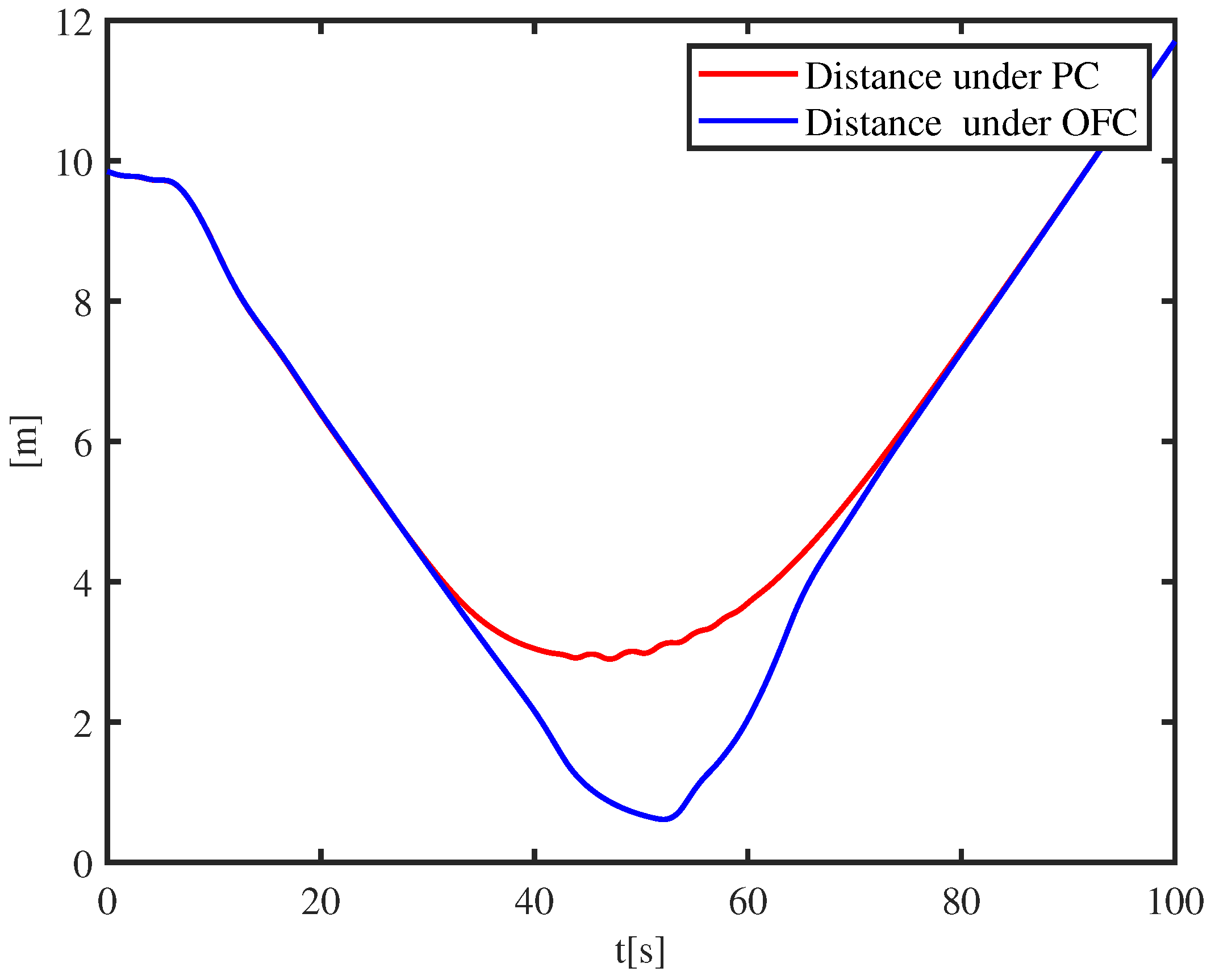
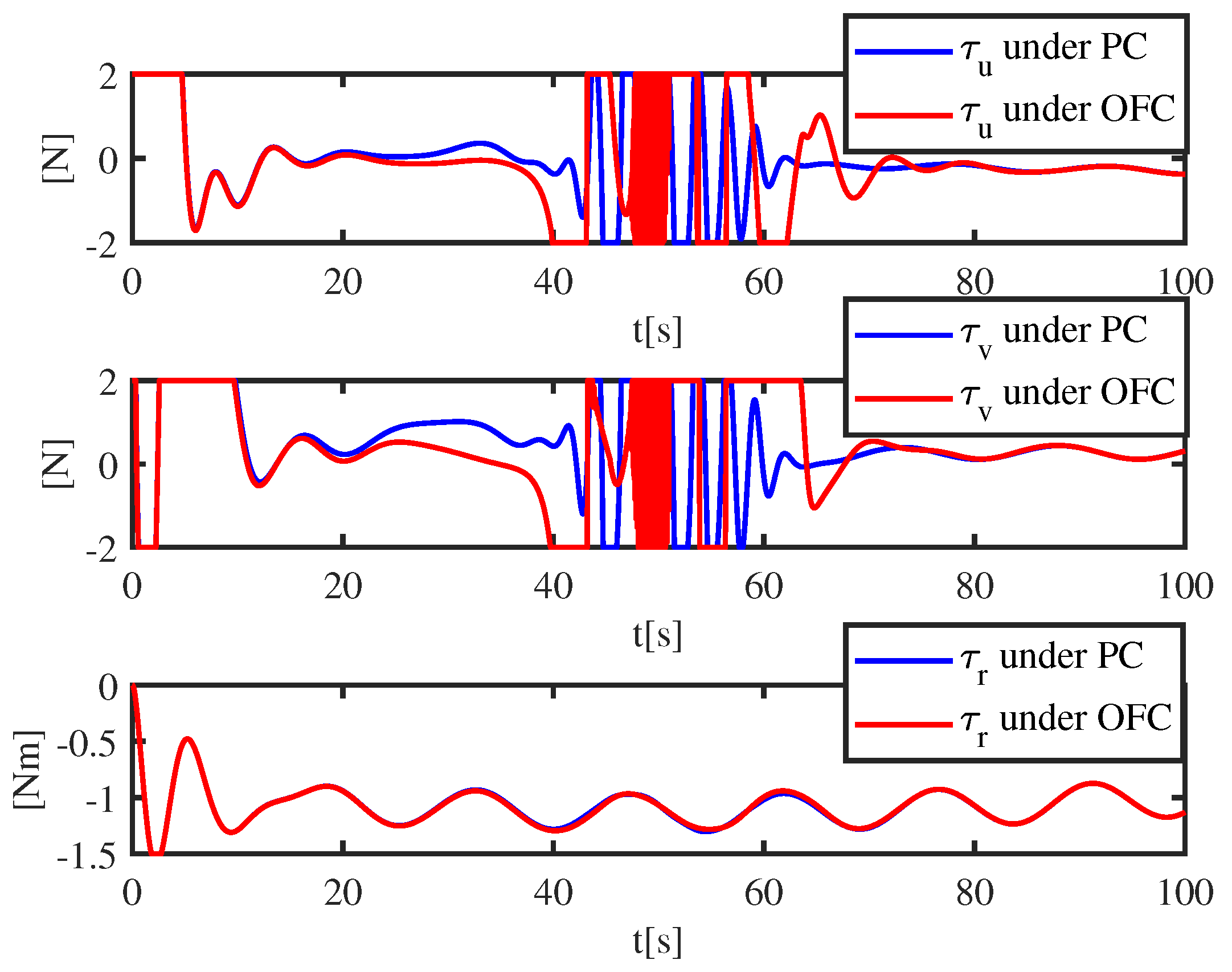
6.3. Comparison Study

To further appraise the performance of the PC, an output feedback tracking controller (OFC) without an auxiliary dynamic system is given by
z 1 = η η d η o
z 2 = ν ^ α ¯ ,
τ c = M ( K 3 z 2 ζ ^ + α ¯ ˙ R T ( ψ ) z 1 ) ,
where the parameters   K 1 K 2 , and  K 3  are same as the proposed controller, and the parameters and structure of the observer are also the same. In the same environmental interference, a non-cooperative ship is considered in trajectory tracking control. The initial position of the non-cooperative ship is set as  [ 4  m,  1  m, 0 rad ] T , and the constant velocity non-cooperative ship is set as  [ 0.1  m/s, 0 m/s, 0 rad/s ] T . The simulation results are shown as Figure 11, Figure 12 and Figure 13. Figure 11 shows the four moments of the trajectory-tracking results, and the dynamic positioning vessel takes evasive action under OFC. At  t = 10  s, the dynamic positioning vessel tracks the desired signal successfully. The non-cooperative ship comes from port side of the dynamic positioning vessel. At  t = 50  s, the non-cooperative ship takes no actions to avoid collisions, and the dynamic positioning vessel makes turns to avoid collisions. However, at  t = 60  s, the dynamic positioning vessel overtakes the non-cooperative ship from its portside. However, unlike the PC, the trajectory of the dynamic positioning vessel has a coincidence with the non-cooperative ship navigation curve. At  t = 100  s, the dynamic positioning vessel moves away from the non-cooperative ship, and the non-cooperative ship sails on the starboard of the dynamic positioning vessel.
Figure 12 shows the time-varying distances between the dynamic positioning vessel and the non-cooperative ship under different controllers. The safe collision-avoidance radii is set to  1.5  m; collisions may happen between the dynamic positioning vessel and non-cooperative ship under OFC. Figure 13 shows that the control inputs suffer from sudden jumps, and the proposed scheme can decrease jitters.

7. Conclusions

This article suggests an output feedback controller for a dynamic positioning vessel with model uncertainty, unknown environmental disturbances, and input constraints. Static obstacles and unknown non-cooperative ships are also considered. An ESO is given, and unknown model dynamics and velocity are simultaneously estimated. The controller is designed based on the ADS and MAPFs. Finally, a mathematical analysis is undertaken to prove that all of the error signals of the system are bounded. Simulation experiments affirm the tracking performance of the proposed controller. This paper proposes an anti-collision controller for the dynamic positioning vessel, and simulations prove that the vessel can avoid the obstacle and navigate itself to the desired trajectory. However, there is no mathematical analysis that shows that the controller can guarantee safety. Finding the best way to solve this problem can be considered as a part of future works.

Author Contributions

Conceptualization, G.X.; methodology, B.Z.; software, B.Z.; validation, B.Z.; and writing—review and editing, B.Z. All authors have read and agreed to the published version of the manuscript.

Funding

This research received no external funding.

Institutional Review Board Statement

This article does not contain any studies with human or animal subjects.

Informed Consent Statement

The study did not involve humans.

Data Availability Statement

The data of this paper are unavailable.

Conflicts of Interest

The authors declare no conflict of interest.

References

  1. Dai, S.L.; Wang, M.; Wang, C. Neural learning control of marine dynamic positioning vessels with guaranteed transient tracking performance. IEEE Trans. Ind. Electron. 2016, 63, 1717–1727. [Google Scholar] [CrossRef]
  2. Gao, S.; Liu, C.; Tuo, Y.; Chen, K.; Zhang, T. Augmented model-based dynamic positioning predictive control for underactuated unmanned surface vessels with dual propellers. Ocean Eng. 2022, 266, 112885. [Google Scholar] [CrossRef]
  3. Sørensen, A.J. A survey of dynamic positioning control systems. Annu. Rev. Control. 2011, 35, 123–136. [Google Scholar] [CrossRef]
  4. Xia, G.Q.; Zhang, B.W. Finite-Time Control of Dynamic Positioning Vessel Based on Disturbance Observer. Math. Probl. Eng. 2022, 2022, 9262457. [Google Scholar] [CrossRef]
  5. Zhang, Z.Y.; Wu, H.T.; Liu, W.X. Effects of mooring line hydrodynamic coefficients and wave parameters on the floating production storage and offloading motions. Desalin. Water Treat. 2021, 239, 278–288. [Google Scholar] [CrossRef]
  6. Liu, X.; Miao, Q.; Wang, X.; Xu, S.; Fan, H. A novel numerical method for the hydrodynamic analysis of floating bodies over a sloping bottom. J. Mar. Sci. Technol. 2021, 26, 1198–1216. [Google Scholar] [CrossRef]
  7. Fan, H.Q.; Miao, Q.M.; Allan, R.M. Wave Loads on the Large Vertical Cylinder with the Conformal Mapping and Series Expansion Method. In Proceedings of the Fourteenth (2020) ISOPE Pacific-Asia Offshore Mechanics Symposium, Dalian, China, 22–25 November 2020. [Google Scholar]
  8. Van, M.; Do, V.T.; Khyam, M.O.; Xuan, P.D. Tracking control of uncertain dynamic positioning vessels with global finite-time convergence. J. Adv. Res. 2021, 241, 109974. [Google Scholar]
  9. Zhu, Y.; Zhang, H.; Li, H.; Zhang, J.; Zhang, D. Optimal Jamming Strategy Against Two-state Switched System. IEEE Commun. Lett. 2022, 13, 1767–1775. [Google Scholar] [CrossRef]
  10. Gao, S.; Xue, J.J. Nonlinear vector model control of underactuated air cushion vehicle based on parameter reduction algorithm. Trans. Inst. Meas. Control. 2021, 43, 1202–1211. [Google Scholar] [CrossRef]
  11. Li, H.; Xu, W.; Zhang, H.; Zhang, J.; Liu, Y. Polynomial regressors based data-driven control for autonomous underwater vehicles. Peer-to-Peer Netw. Appl. 2020, 13, 1767–1775. [Google Scholar] [CrossRef]
  12. Fang, M.C.; Zhuo, Y.Z.; Lee, Z.Y. The application of the self-tuning neural network PID controller on the ship roll reduction in random waves. Ocean. Eng. 2010, 37, 529–538. [Google Scholar] [CrossRef]
  13. Larrazabal, J.M.; Penas, M.S. Intelligent rudder control of an unmanned surface vessel. Expert Syst. Appl. 2016, 55, 106–117. [Google Scholar] [CrossRef]
  14. Ishaque, K.; Abdullah, S.; Ayob, S.; Salam, Z. A simplified approach to design fuzzy logic controller for an underwater vehicle. Ocean Eng. 2011, 38, 271–284. [Google Scholar] [CrossRef]
  15. Abdelaal, M.; Fränzle, M.; Hahn, A. Nonlinear model predictive control for trajectory tracking and collision avoidance of underactuated vessels with disturbances. Ocean Eng. 2018, 160, 168–180. [Google Scholar] [CrossRef]
  16. Ashrafiuon, H.; Muske, K.; McNinch, L. Sliding-mode tracking control of dynamic positioning vessels. IEEE Trans. Ind. Electron. 2008, 55, 4004–4012. [Google Scholar] [CrossRef]
  17. Xia, G.; Xia, X.; Zhao, B.; Sun, C.; Sun, X. A solution to leader following of underactuated dynamic positioning vessel s with actuator magnitude and rate limits. Int. J. Adapt. Control. Signal Process. 2021, 35, 1860–1878. [Google Scholar] [CrossRef]
  18. Xia, G.Q.; Xia, X.M.; Sun, X.X. Formation tracking control for underactuated surface vehicles with actuator magnitude and rate saturations. Ocean Eng. 2022, 260, 111935. [Google Scholar] [CrossRef]
  19. Zhu, H.; Yu, H.M.; Guo, C. Finite time PAILOS based path following control of underactuated marine surface vessel with input saturation. ISA Trans. 2022, 135, 66–77. [Google Scholar] [CrossRef]
  20. Xia, G.; Xia, X.; Bo, Z.; Sun, X.; Sun, C. Event-Triggered Controller Design for Autopilot with Input Saturation. Math. Probl. Eng. 2020, 2020, 5362895. [Google Scholar] [CrossRef]
  21. Zhu, G.; Du, J. Global Robust Adaptive Trajectory Tracking Control for dynamic positioning ships Under Input Saturation. IEEE J. Ocean. Eng. 2020, 45, 442–450. [Google Scholar] [CrossRef]
  22. Qin, H.; Li, C.; Sun, Y.; Li, X.; Du, Y.; Deng, Z. Finite-time trajectory tracking control of unmanned surface vessel with error constraints and input saturations. J. Frankl. Inst. 2020, 357, 11472–11495. [Google Scholar] [CrossRef]
  23. Qin, H.; Li, C.; Sun, Y.; Wang, N. Adaptive trajectory tracking algorithm of unmanned dynamic positioning vessel based on anti-windup compensator with full-state constraints. Ocean Eng. 2020, 200, 106906. [Google Scholar] [CrossRef]
  24. Xia, G.; Xia, X.; Zhao, B.; Sun, C.; Sun, X. Distributed Tracking Control for Connectivity-Preserving and Collision-Avoiding Formation Tracking of Underactuated Surface Vessels with Input Saturation. Appl. Sci. 2020, 10, 3372. [Google Scholar] [CrossRef]
  25. Zeng, Z.; Yu, H.; Guo, C.; Yan, Z. Finite-time coordinated formation control of discrete-time multi-AUV with input saturation under alterable weighted topology and time-varying delay. Ocean Eng. 2022, 266, 112881. [Google Scholar] [CrossRef]
  26. Tam, C.K.; Bucknall, R. Cooperative path-planning algorithm for marine dynamic positioning vessels. Ocean Eng. 2013, 57, 25–33. [Google Scholar] [CrossRef]
  27. Li, Y.; Zheng, J. Real-time collision avoidance planning for unmanned surface vessels based on field theory. ISA Trans. 2020, 106, 233–242. [Google Scholar] [CrossRef]
  28. Wang, W.M.; Du, J.L.; Tao, Y.H. A dynamic collision avoidance solution scheme of unmanned surface vessels based on proactive velocity obstacle and set-based guidance. Ocean Eng. 2022, 248, 110794. [Google Scholar]
  29. Park, J.W. Improved Collision Avoidance Method for Autonomous Surface Vessels Based on Model Predictive Control Using Particle Swarm Optimization. Int. J. Fuzzy Log. Intell. Syst. 2021, 21, 378–390. [Google Scholar] [CrossRef]
  30. Peng, Z.; Wang, D.; Li, T.; Han, M. Output-Feedback Cooperative Formation Maneuvering of Autonomous Surface Vehicles With Connectivity Preservation and Collision Avoidance. IEEE Trans. Cybern. 2020, 50, 2527–2535. [Google Scholar] [CrossRef]
  31. Park, B.S.; Yoo, S.J. An error transformation approach for connectivity-preserving and collision-avoiding formation tracking of networked uncertain underactuated dynamic positioning vessels. IEEE Trans. Cybern. 2019, 49, 353–359. [Google Scholar] [CrossRef]
  32. Fossen, T.I.; Strand, J.P. Passive nonlinear observer design for ships using Lyapunov methods: Full-Scale experiments with a supply vessel. Automatica 1999, 35, 3–16. [Google Scholar] [CrossRef]
  33. Liang, X.; Qu, X.; Wang, N.; Li, Y.; Zhang, R. Swarm control with collision avoidance for multiple underactuated surface vehicles. Ocean Eng. 2019, 191, 106516. [Google Scholar] [CrossRef]
  34. Xia, G.Q.; Xia, X.M.; Sun, X.X. Formation control with collision avoidance for underactuated surface vehicles. Asian J. Control. 2022, 24, 2244–2257. [Google Scholar] [CrossRef]
  35. Kowalczyk, W.; Michaek, M.; Kozowski, K. Trajectory tracking control and obstacle avoidance for a differentially driven mobile robot. IFAC-World Congr. 2011, 41, 1058–1063. [Google Scholar] [CrossRef]
  36. Xia, G.; Sun, C.; Zhao, B.; Xia, X.; Sun, X. Neuroadaptive Distributed Output Feedback Tracking Control for Multiple Marine Surface Vessels With Input and Output Constraints. IEEE Access 2019, 7, 123076–123085. [Google Scholar] [CrossRef]
  37. Kowalczyk, W.; Michaek, M.; Kozowski, K. Collaborative collision avoidance for Maritime Autonomous dynamic positioning ships: A review. IFAC-World Congr. 2011, 41, 1058–1063. [Google Scholar]
  38. Skjetne, R.; Fossen, T.I.; Kokotovi, P.V. Adaptive maneuvering, with experiments, for a model ship in a marine control laboratory. Automatica 2005, 41, 289–298. [Google Scholar] [CrossRef]
Figure 1. The diagram of the proposed output feedback controller.
Jmse 11 00811 g001
Figure 2. Trajectory tracking control under four cases (the green circle denotes obstacle).
Jmse 11 00811 g002
Figure 3. The distances between dynamic positioning vessel and obstacle under four cases.
Jmse 11 00811 g003
Figure 4. z 1 T z 1  under four cases.
Jmse 11 00811 g004
Figure 5. Velocity estimation.
Jmse 11 00811 g005
Figure 6. Unknown function and estimation.
Jmse 11 00811 g006
Figure 7. Control inputs.
Jmse 11 00811 g007
Figure 8. Four moments of trajectory tracking control.
Jmse 11 00811 g008
Figure 9. The distance between dynamic positioning vessel and non-cooperative ship.
Jmse 11 00811 g009
Figure 10. Control inputs under non-cooperative ship.
Jmse 11 00811 g010
Figure 11. Four moments of trajectory tracking control under OFC.
Jmse 11 00811 g011
Figure 12. The distances between dynamic positioning vessel and non-cooperative ship under different controllers.
Jmse 11 00811 g012
Figure 13. Input signals under different controllers.
Jmse 11 00811 g013
Table 1. Design simulations.
Simulation Scenario   η ( 0 )   ν d ( t )   P o
Case 1 [ 2  m,  2  m, 0 rad ] T [ 0.2  m/s, 0 m/s, 0 rad/s ] T [ 10  m,  1  m ] T
Case 2 [ 2  m,  2  m, 0 rad ] T [ 0.2  m/s, 0 m/s, 0 rad/s ] T [ 10  m, 1  m ] T
Case 3 [ 8  m,  10  m, 0 rad ] T [ 0  m/s,  0.2  m/s, 0 rad/s ] T [ 10  m,  1  m ] T
Case 4 [ 8  m,  10  m, 0 rad ] T [ 0  m/s,  0.2  m/s, 0 rad/s ] T [ 10  m,  1  m ] T
Disclaimer/Publisher’s Note: The statements, opinions and data contained in all publications are solely those of the individual author(s) and contributor(s) and not of MDPI and/or the editor(s). MDPI and/or the editor(s) disclaim responsibility for any injury to people or property resulting from any ideas, methods, instructions or products referred to in the content.

