
New Methodology for Shoreline Extraction Using Optical and Radar (SAR) Satellite Imagery

 ,
,  , , , , and
Abstract
:1. Introduction and State of the Art
2. Materials and Methods
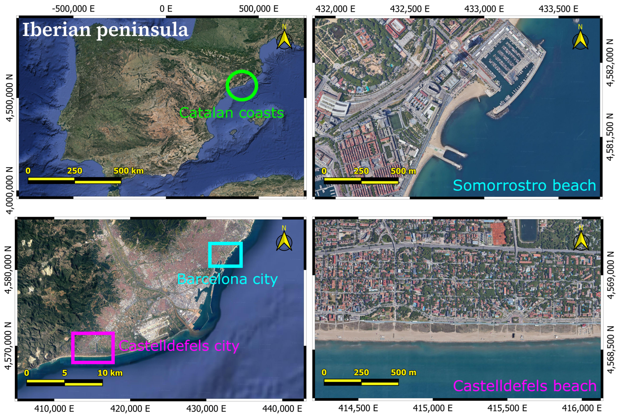
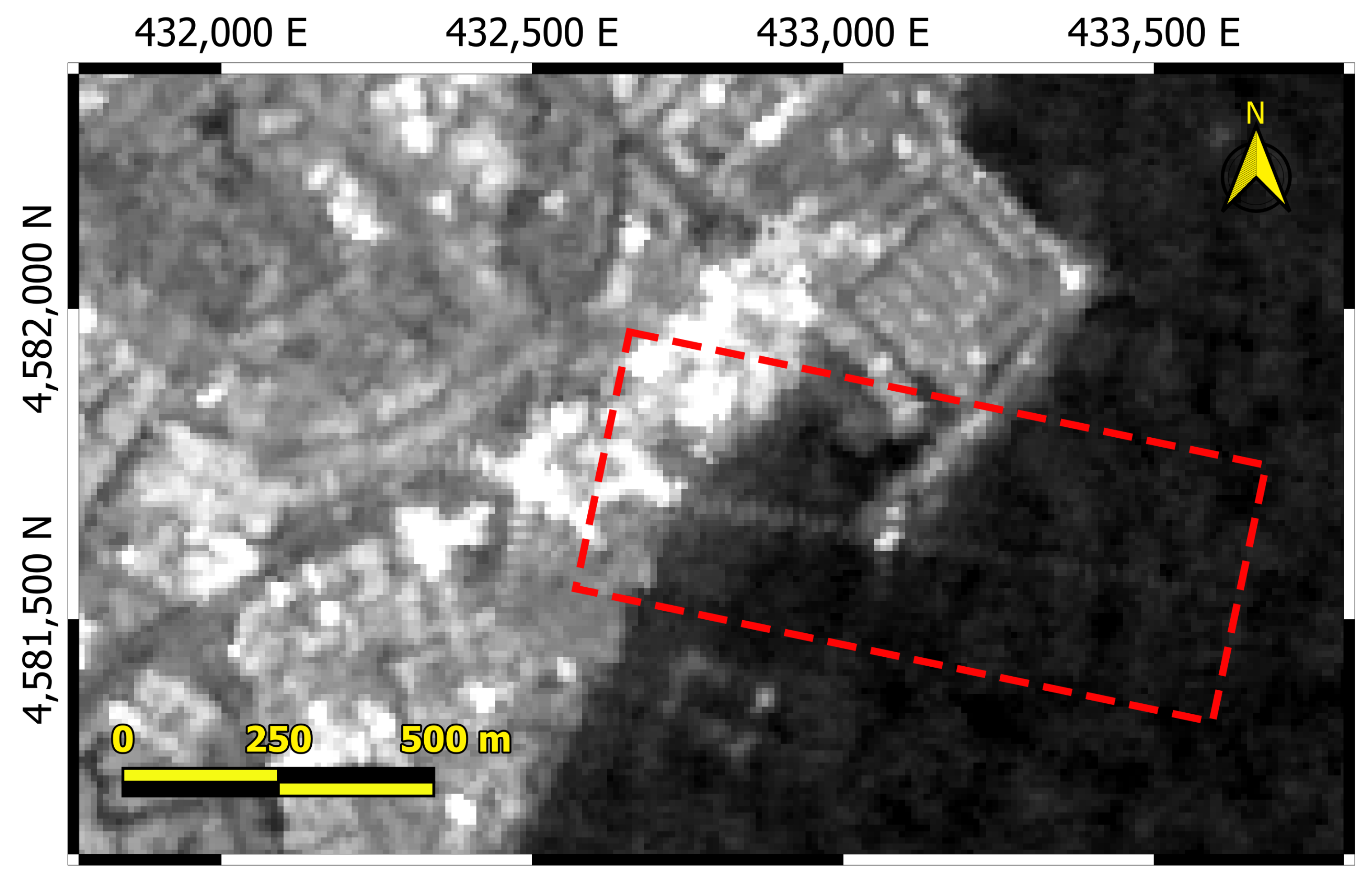
2.1. Study Areas
2.2. Sentinel-1 and -2 Imagery and GNSS Data Sets
2.3. Pre-Processing of S1 and S2 Images
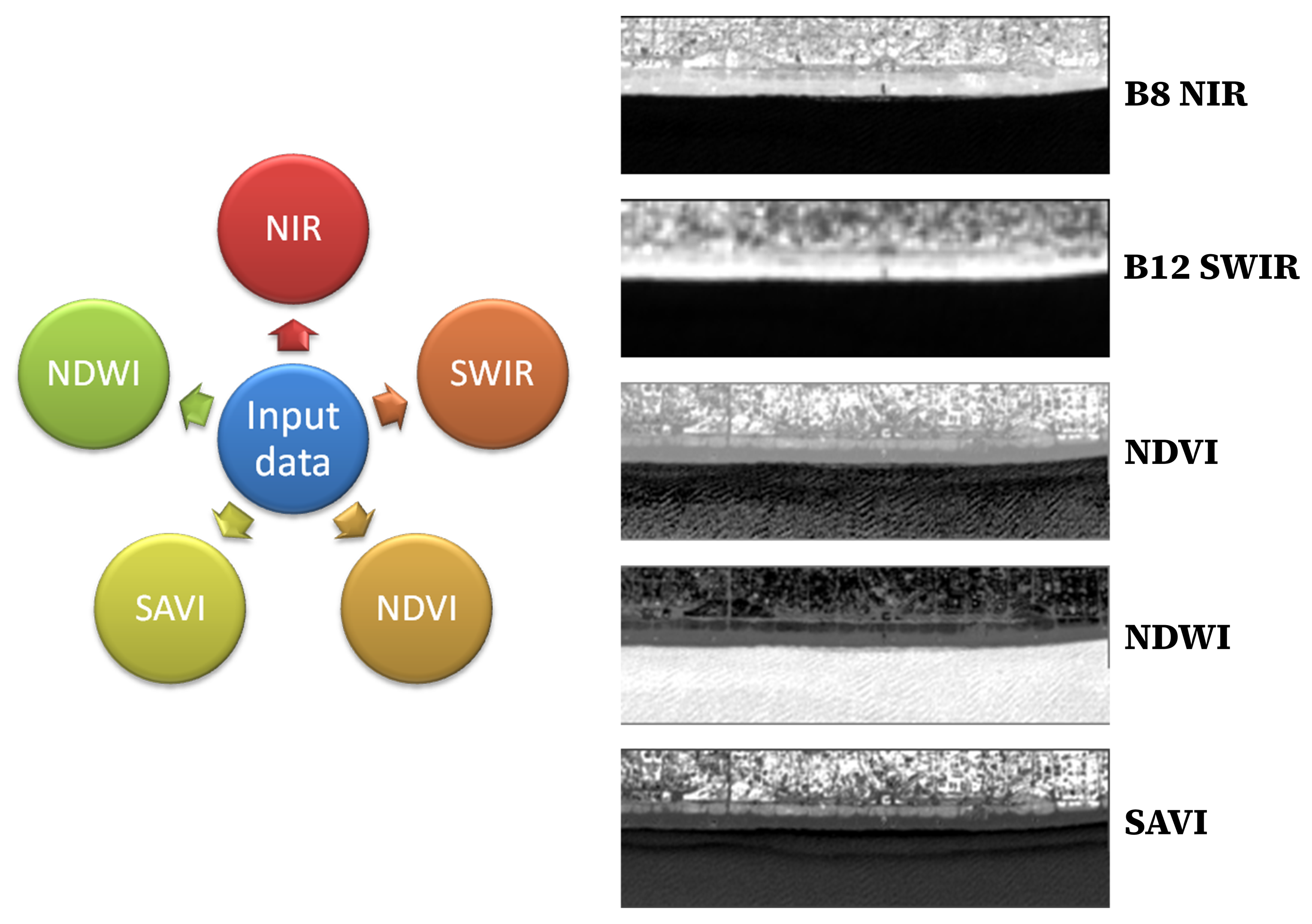
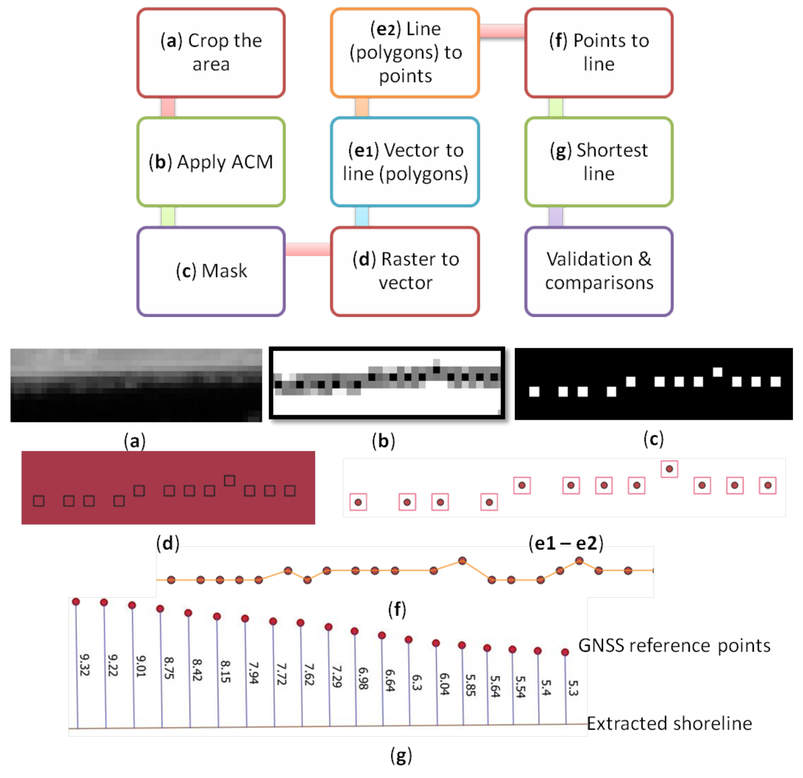
2.4. New Methodology for Shoreline Extraction
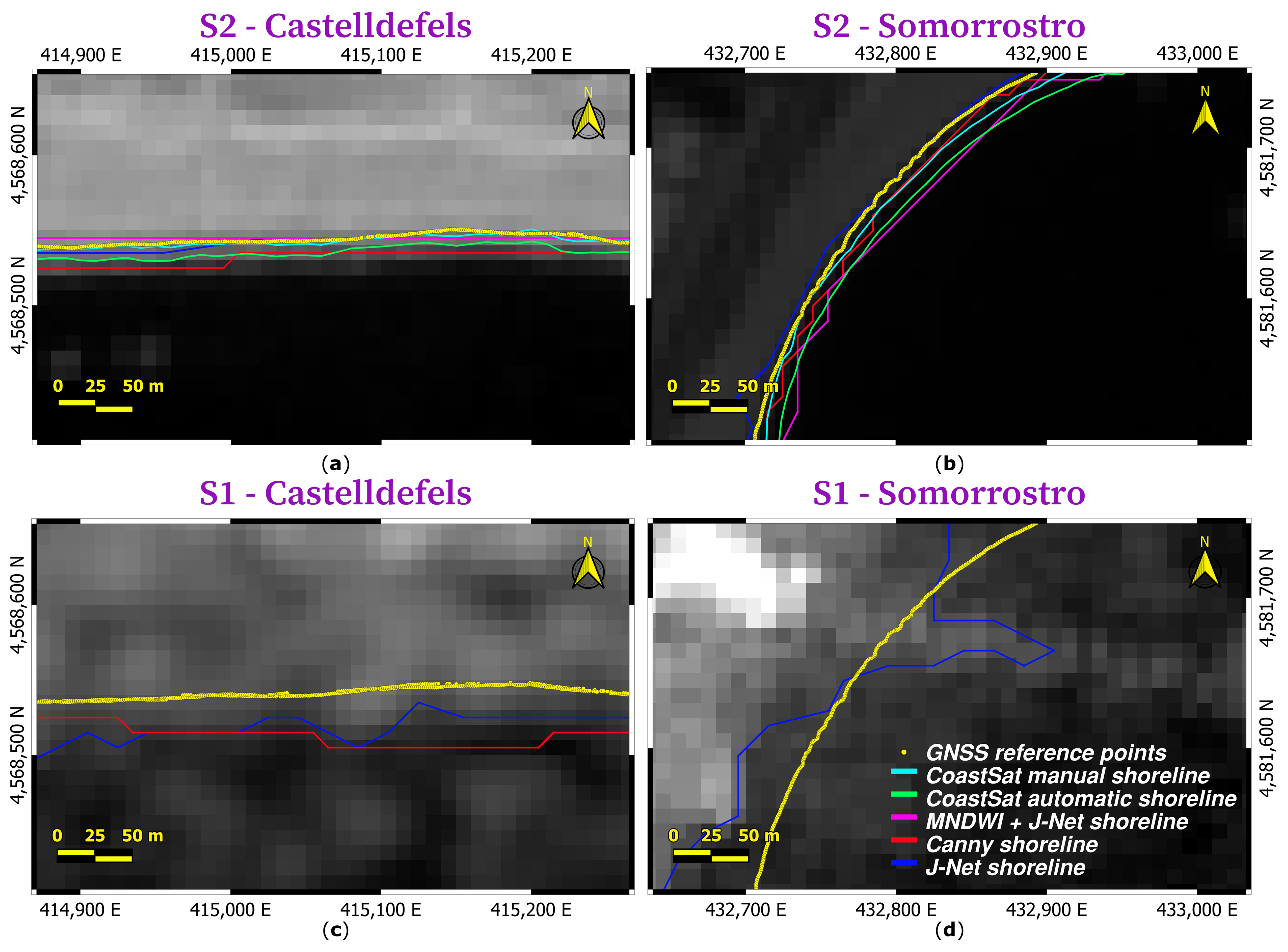
2.5. Alternative Detection Methods
3. Results
3.1. Results of the New Methodology
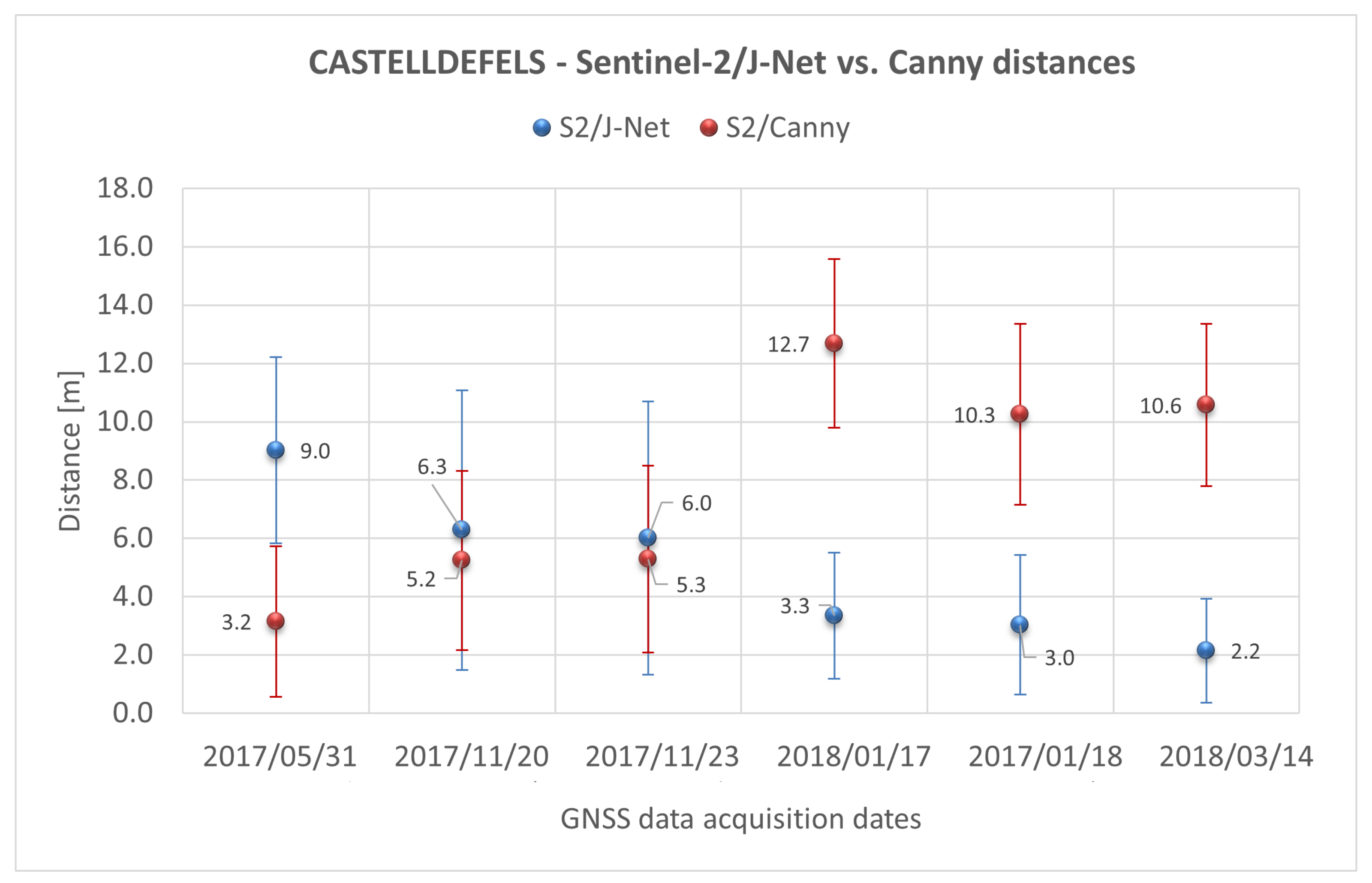
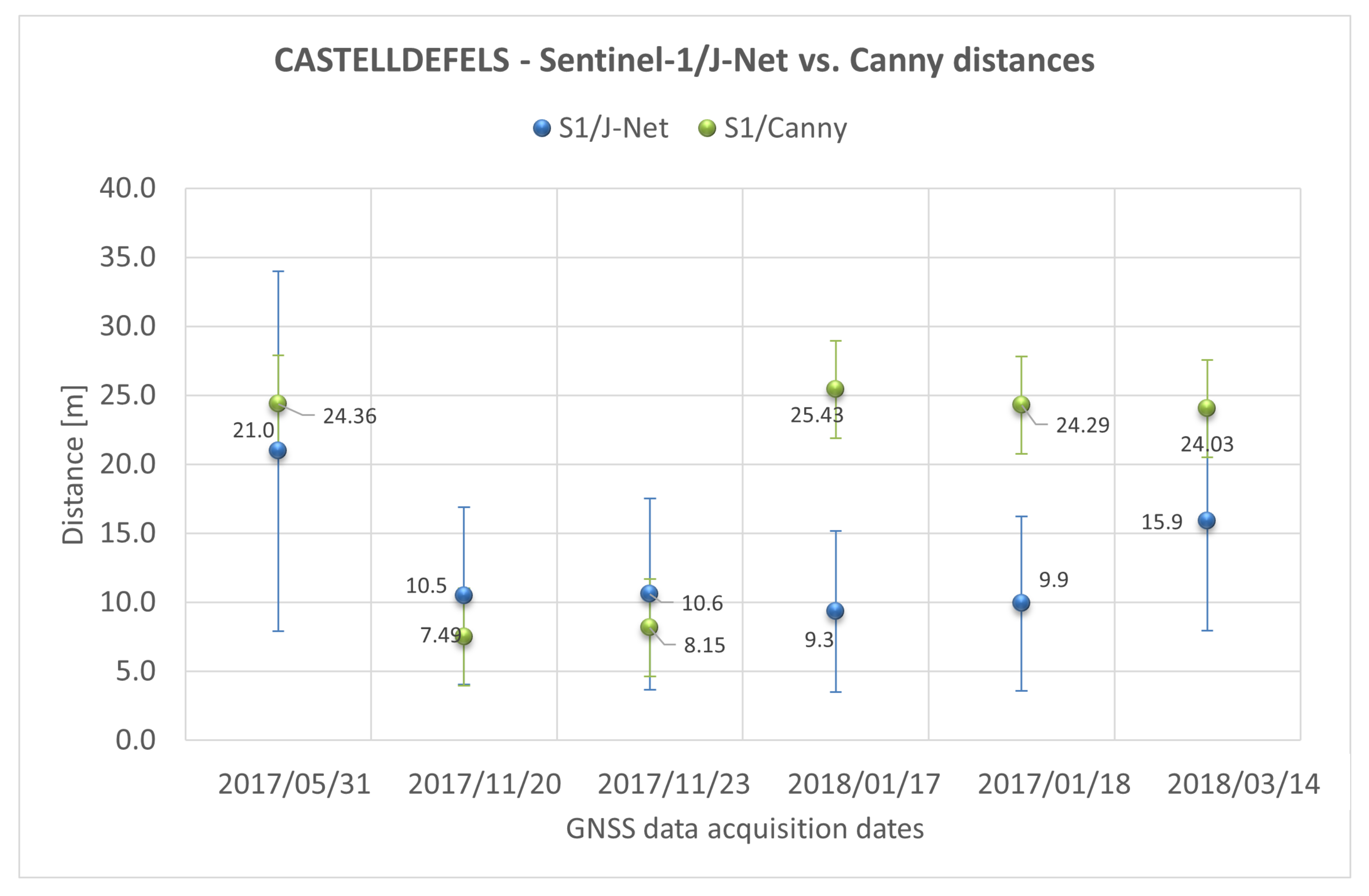
3.2. Comparison with Canny Algorithm
3.3. Comparison with CoastSat Tool
4. Discussion
4.1. Role of the Oceanographic Conditions on the Obtained Errors
4.2. Analysis of the Obtained Results
5. Conclusions
Author Contributions
Funding
Institutional Review Board Statement
Informed Consent Statement
Data Availability Statement
Conflicts of Interest
Abbreviations
| ACM | Active Connection Matrix |
| AWEI | Automated Water Extraction Index |
| DEM | Digital Elevation Model |
| dGPS | Differential Global Positioning System |
| EC | European Commission |
| EO | Earth Observation |
| EPSG | European Petroleum Survey Group |
| ESA | European Space Agency |
| GEE | Google Earth Engine |
| GNSS | Global Navigation Satellite System |
| GRD | Ground Range Detected |
| IW | Interferometric Wide |
| MNDWI | Modified Normalized Difference Water Index |
| NDVI | Normalized Difference Vegetation Index |
| NDWI | Normalized Difference Water Index |
| NIR | Near InfraRed |
| QGIS | Quantum Geographic Information System |
| S1 | Sentinel-1 |
| S2 | Sentinel-2 |
| SAR | Synthetic Aperture Radar |
| SAVI | Soil Adjusted Vegetation Index |
| SNAP | Sentinel Application Platform |
| SWAN | Simulating WAves Nearshore |
| SWIR | Short Wave InfraRed |
| UTM | Universal Transverse Mercator |
| WGS84 | World Geodetic System 84 |
| WI | Water Index |
Appendix A. Graphical Comparison between the Results


References
- Small, C.; Nicholls, R.J. A global analysis of human settlement in coastal zones. J. Coast. Res. 2003, 19, 584–599. [Google Scholar]
- Rajib, S. Chapter 1—Global Coasts in the Face of Disasters. In Coastal Management; Krishnamurthy, R.R., Jonathan, M.P., Srinivasalu, S., Glaeser, B., Eds.; Academic Press: Cambridge, MA, USA, 2019; pp. 1–4. Available online: https://www.sciencedirect.com/science/article/pii/B9780128104736000017?via%3Dihub (accessed on 21 June 2022).
- Neumann, B.; Vafeidis, A.T.; Zimmermann, J.; Nicholls, R.J. Future coastal population growth and exposure to sea-level rise and coastal ooding-a global assessment. PLoS ONE 2015, 10, e0118571. [Google Scholar] [CrossRef] [PubMed] [Green Version]
- Oppenheimer, M.; Glavovic, B.C.; Hinkel, J.; Wal, R.v.; Magnan, A.K.; Abd-Elgawad, A.; Cai, R.; Cifuentes-Jara, M.; DeConto, R.M.; Ghosh, T.; et al. Sea Level Rise and Implications for Low-Lying Islands, Coasts and Communities. In IPCC Special Report on the Ocean and Cryosphere in a Changing Climate; Cambridge University Press: Cambridge, UK; New York, NY, USA, 2019; pp. 321–445. [Google Scholar] [CrossRef]
- Frederikse, T.; Landerer, F.W.; Caron, L.; Adhikari, S.; Parkes, D.; Humphrey, V.; Dangendorf, S.; Hogarth, P.; Zanna, L.; Cheng, L.; et al. The causes of sea-level rise since 1900. Nature 2020, 584, 393–397. [Google Scholar] [CrossRef] [PubMed]
- Mentaschi, L.; Vousdoukas, M.I.; Pekel, J.-F.; Voukouvalas, E.; Feyen, L. Global long-term observations of coastal erosion and accretion. Sci. Rep. 2018, 8, 12876. [Google Scholar] [CrossRef] [Green Version]
- Jiménez, J.A.; Valdemoro, H.I. Shoreline evolution and its management implications in beaches along the Catalan coast. In The Spanish Coastal Systems: Dynamic Processes, Sediments and Management; Springer: Berlin/Heidelberg, Germany, 2019; pp. 745–764. [Google Scholar]
- Pranzini, E.; Wetzel, L.; Williams, A.T. Aspects of coastal erosion and protection in Europe. J. Coast. Conserv. 2015, 19, 445–459. [Google Scholar] [CrossRef]
- Boak, E.H.; Turner, I.L. Shoreline definition and detection: A review. J. Coast. Res. 2005, 21, 688–703. [Google Scholar] [CrossRef] [Green Version]
- Pugliano, G.; Robustelli, U.; Di Luccio, D.; Mucerino, L.; Benassai, G.; Montella, R. Statistical deviations in shoreline detection obtained with direct and remote observations. J. Mar. Sci. Eng. 2019, 7, 137. [Google Scholar] [CrossRef] [Green Version]
- Dominici, D.; Zollini, S.; Alicandro, M.; Della Torre, F.; Buscema, P.M.; Baiocchi, V. High Resolution Satellite Images for Instantaneous Shoreline Extraction Using New Enhancement Algorithms. Geosciences 2019, 9, 123. [Google Scholar] [CrossRef] [Green Version]
- Goncalves, G.; Duro, N.; Sousa, E.; Figueiredo, I. Automatic extraction of tide-coordinated shoreline using open source software and Landsat imagery. Int. Arch. Photogramm. Remote Sens. Spat. Inf. Sci. 2015, 40, 953. [Google Scholar] [CrossRef] [Green Version]
- Pardo-Pascual, J.E.; Sánchez-García, E.; Almonacid-Caballer, J.; Palomar-Vázquez, J.M.; Priego De Los Santos, E.; Fernández-Sarría, A.; Balaguer-Beser, Á. Assessing the accuracy of automatically extracted shorelines on microtidal beaches from Landsat 7, Landsat 8 and Sentinel-2 imagery. Remote Sens. 2018, 10, 326. [Google Scholar] [CrossRef] [Green Version]
- DaSilva, M.; Miot da Silva, G.; Hesp, P.A.; Bruce, D.; Keane, R.; Moore, C. Assessing Shoreline Change using Historical Aerial and RapidEye Satellite Imagery (Cape Jaffa, South Australia). J. Coast. Res. 2021, 37, 468–483. [Google Scholar] [CrossRef]
- Wei, X.; Zheng, W.; Xi, C.; Shang, S. Shoreline Extraction in SAR Image Based on Advanced Geometric Active Contour Model. Remote Sens. 2021, 13, 642. [Google Scholar] [CrossRef]
- Simarro, G.; Bryan, K.R.; Guedes, R.M.; Sancho, A.; Guillen, J.; Coco, G. On the use of variance images for runup and shoreline detection. Coast. Eng. 2015, 99, 136–147. [Google Scholar] [CrossRef]
- Ribas, F.; Simarro, G.; Arriaga, J.; Luque, P. Automatic shoreline detection from video images by combining information from different methods. Remote Sens. 2020, 12, 3717. [Google Scholar] [CrossRef]
- Vitousek, S.; Buscombe, D.; Vos, K.; Barnard, P.L.; Ritchie, A.; Warrick, J. The future of coastal monitoring through satellite remote sensing. Camb. Prism. Coast. Futures 2022, 1, e10. [Google Scholar] [CrossRef]
- Braga, F.; Tosi, L.; Prati, C.; Alberotanza, L. Shoreline detection: Capability of COSMO-SkyMed and high-resolution multispectral images. Eur. J. Remote Sens. 2013, 46, 837–853. [Google Scholar] [CrossRef]
- Dammann, D.O.; Eriksson, L.E.; Mahoney, A.R.; Eicken, H.; Meyer, F.J. Mapping pan-Arctic landfast sea ice stability using Sentinel-1 interferometry. Cryosphere 2019, 13, 557–577. [Google Scholar] [CrossRef] [Green Version]
- Chaturvedi, S.K.; Banerjee, S.; Lele, S. An assessment of oil spill detection using Sentinel-1 SAR-C images. J. Ocean Eng. Sci. 2019, 5, 116–135. [Google Scholar] [CrossRef]
- Wang, Y.; Wang, C.; Zhang, H. Combining a single shot multibox detector with transfer learning for ship detection using Sentinel-1 SAR images. Remote Sens. Lett. 2018, 9, 780–788. [Google Scholar] [CrossRef]
- Forkuor, G.; Zoungrana, J.B.; Dimobe, K.; Ouattara, B.; Vadrevu, K.P.; Tondoh, J.E. Above-ground biomass mapping in West African dryland forest using Sentinel-1 and 2 datasets—A case study. Remote Sens. Environ. 2020, 236, 111496. [Google Scholar] [CrossRef]
- Steinhausen, M.J.; Wagner, P.D.; Narasimhan, B.; Waske, B. Combining Sentinel-1 and Sentinel-2 data for improved land use and land cover mapping of monsoon regions. Int. J. Appl. Earth Obs. Geoinf. 2018, 73, 595–604. [Google Scholar] [CrossRef]
- Van Tricht, K.; Gobin, A.; Gilliams, S.; Piccard, I. Synergistic use of radar Sentinel-1 and optical Sentinel-2 imagery for crop mapping: A case study for Belgium. Remote Sens. 2018, 10, 1642. [Google Scholar] [CrossRef] [Green Version]
- Montalti, R.; Solari, L.; Bianchini, S.; Del Soldato, M.; Raspini, F.; Casagli, N. A Sentinel-1-based clustering analysis for geo-hazards mitigation at regional scale: A case study in Central Italy. Geomat. Nat. Hazards Risk 2019, 10, 2257–2275. [Google Scholar] [CrossRef] [Green Version]
- Thanh Noi, P.; Kappas, M. Comparison of random forest, k-nearest neighbor, and support vector machine classifiers for land cover classification using Sentinel-2 imagery. Sensors 2018, 18, 18. [Google Scholar] [CrossRef] [PubMed] [Green Version]
- Drusch, M.; Del Bello, U.; Carlier, S.; Colin, O.; Fernandez, V.; Gascon, F.; Hoersch, B.; Isola, C.; Laberinti, P.; Martimort, P.; et al. Sentinel-2: ESA’s optical high-resolution mission for GMES operational services. Remote Sens. Environ. 2012, 120, 25–36. [Google Scholar] [CrossRef]
- Veloso, A.; Mermoz, S.; Bouvet, A.; Le Toan, T.; Planells, M.; Dejoux, J.-F.; Ceschia, E. Understanding the temporal behavior of crops using Sentinel-1 and Sentinel-2-like data for agricultural applications. Remote Sens. Environ. 2017, 199, 415–426. [Google Scholar] [CrossRef]
- El Hajj, M.; Baghdadi, N.; Zribi, M.; Bazzi, H. Synergic use of Sentinel-1 and Sentinel-2 images for operational soil moisture mapping at high spatial resolution over agricultural areas. Remote Sens. 2017, 9, 1292. [Google Scholar] [CrossRef] [Green Version]
- Demir, N.; Kaynarca, M.; Oy, S. Extraction of coastlines with fuzzy approach using SENTINEL-1 SAR image. Int. Arch. Photogramm. Remote Sens. Spat. Inf. Sci. 2016, 41, 747. [Google Scholar] [CrossRef] [Green Version]
- Suhendra, S.; Setiawan, C.A.; Wibawa, T.A.; Borneo, B.B. Coastline change analysis on Bali island using Sentinel-1 satellite imagery. Int. J. Remote Sens. Earth Sci. (IJReSES) 2021, 18, 63–72. [Google Scholar] [CrossRef]
- López-Caloca, A.A.; Monsiváis-Huertero, A.; López-Amaya, J. Sentinel-1 observation for shoreline delineation applied to Mexico’s Coast. Geocarto Int. 2022, 37, 16462–16491. [Google Scholar] [CrossRef]
- Vos, K.; Splinter, K.D.; Harley, M.D.; Simmons, J.A.; Turner, I.L. CoastSat: A Google Earth Engine-enabled Python toolkit to extract shorelines from publicly available satellite imagery. Environ. Model. Softw. 2019, 122, 104528. [Google Scholar] [CrossRef]
- Almeida, L.P.; de Oliveira, I.E.; Lyra, R.; Dazzi, R.L.S.; Martins, V.G.; da Fontoura Klein, A.H. Coastal analyst system from space imagery engine (CASSIE): Shoreline management module. Environ. Model. Softw. 2021, 140, 105033. [Google Scholar] [CrossRef]
- Sánchez-García, E.; Palomar-Vázquez, J.; Pardo-Pascual, J.; Almonacid-Caballer, J.; Cabezas-Rabadán, C.; Gómez-Pujol, L. An efficient protocol for accurate and massive shoreline definition from mid-resolution satellite imagery. Coast. Eng. 2020, 160, 103732. [Google Scholar] [CrossRef]
- Pucino, N.; Kennedy, D.M.; Young, M.; Ierodiaconou, D. Assessing the accuracy of Sentinel-2 instantaneous subpixel shorelines using synchronous UAV ground truth surveys. Remote Sens. Environ. 2022, 282, 113293. [Google Scholar] [CrossRef]
- McFeeters, S.K. The use of the normalized difference water index (NDWI) in the delineation of open water features. Int. J. Remote Sens. 1996, 17, 1425–1432. [Google Scholar] [CrossRef]
- Xu, H. Modification of normalised difference water index (NDWI) to enhance open water features in remotely sensed imagery. Int. J. Remote Sens. 2006, 27, 3025–3033. [Google Scholar] [CrossRef]
- Vos, K.; Harley, M.D.; Splinter, K.D.; Simmons, J.A.; Turner, I.L. Sub-annual to multi-decadal shoreline variability from publicly available satellite imagery. Coast. Eng. 2019, 150, 160–174. [Google Scholar] [CrossRef]
- Feyisa, G.L.; Meilby, H.; Fensholt, R.; Proud, S.R. Automated water extraction index: A new technique for surface water mapping using landsat imagery. Remote Sens. Environ. 2014, 140, 23–35. [Google Scholar] [CrossRef]
- Fisher, A.; Flood, N.; Danaher, T. Comparing landsat water index methods for automated water classification in eastern Australia. Remote Sens. Environ. 2016, 175, 167–182. [Google Scholar] [CrossRef]
- Ferrentino, E.; Buono, A.; Nunziata, F.; Marino, A.; Migliaccio, M. On the use of multipolarization satellite SAR data for coastline extraction in harsh coastal environments: The case of Solway Firth. IEEE J. Sel. Top. Appl. Earth Obs. Remote Sens. 2020, 14, 249–257. [Google Scholar] [CrossRef]
- Zollini, S.; Alicandro, M.; Cuevas-González, M.; Baiocchi, V.; Dominici, D.; Buscema, P.M. Shoreline extraction based on an active connection matrix (ACM) image enhancement strategy. J. Mar. Sci. Eng. 2020, 8, 9. [Google Scholar] [CrossRef] [Green Version]
- Kelly, J.; Gontz, A. Using GNSS-surveyed intertidal zones to determine the validity of shorelines automatically mapped by Landsat water indices. Int. J. Appl. Earth Obs. Geoinf. 2018, 65, 92–104. [Google Scholar]
- Maglione, P.; Parente, C.; Vallario, A. High resolution satellite images to reconstruct recent evolution of domitian coastline. Am. J. Appl. Sci. 2015, 12, 506. [Google Scholar] [CrossRef] [Green Version]
- ESA—European Space Agency (n.d.). Sentinel-1—Overview—Sentinel Online. Available online: https://sentinel:esa:int/web/sentinel/missions/sentinel-1/overview (accessed on 19 May 2020).
- ESA—European Space Agency (n.d.). Sentinel-2—Overview—Sentinel Online. Available online: https://sentinel:esa:int/web/sentinel/missions/sentinel-2/overview (accessed on 21 May 2020).
- Lee, J.; Jurkevich, L.; Dewaele, P.; Wambacq, P.; Oosterlinck, A. Speckle filtering of synthetic aperture radar images: A review. Remote Sens. Rev. 1994, 8, 313–340. [Google Scholar] [CrossRef]
- Lopes, A.; Nezry, E.; Touzi, R.; Laur, H. Structure detection and statistical adaptive speckle filtering in SAR images. Int. J. Remote Sens. 1993, 14, 1735–1758. [Google Scholar] [CrossRef]
- Wang, P.; Zhang, H.; Patel, V.M. SAR image despeckling using a convolutional neural network. IEEE Signal Process. Lett. 2017, 24, 1763–1767. [Google Scholar] [CrossRef] [Green Version]
- Sivaranjani, R.; Roomi, S.; Senthilarasi, M. Speckle noise removal in SAR images using Multi-Objective PSO (MOPSO) algorithm. Appl. Soft Comput. 2019, 76, 671–681. [Google Scholar] [CrossRef]
- Buscema, P.M. Sistemi ACM e Imaging Diagnostico: Le Immagini Mediche Come Matrici Attive di Connessioni; Springer Science & Business Media: New York, NY, USA, 2006. [Google Scholar]
- Buscema, M.; Catzola, L.; Grossi, E. Images as active connection matrixes: The J-net system. Int. J. Intell. Comput. Med. Sci. Image Process. 2008, 2, 27–53. [Google Scholar] [CrossRef]
- Buscema, M.; Grossi, E. J-Net System: A New Paradigm for Artificial Neural Networks Applied to Diagnostic Imaging. In Applications of Mathematics in Models, Artificial Neural Networks and Arts; Publishing House: Dordrecht, The Netherlands, 2010; pp. 431–455. [Google Scholar]
- Canny, J. A computational approach to edge detection. IEEE Trans. Pattern Anal. Mach. Intell. 1986, 6, 679–698. [Google Scholar] [CrossRef]
- Sahir, S. Canny Edge Detection Step by Step in Python—Computer Vision. 2019. Available online: https://towardsdatascience:com/canny-edge-detection-step-by-step-in-python-computer-vision-b49c3a2d8123 (accessed on 10 October 2020).
- Github CoastSat. Available online: https://github.com/kvos/CoastSat (accessed on 16 November 2022).
- Castelle, B.; Masselink, G.; Scott, T.; Stokes, C.; Konstantinou, A.; Marieu, V.; Bujan, S. Satellite-derived shoreline detection at a high-energy meso-macrotidal beach. Geomorphology 2021, 383, 107707. [Google Scholar] [CrossRef]
- Sancho-García, A. Beach Inundation and Morphological Changes during Storms Using Video Monitoring Techniques. Ph.D. Thesis, Universitat Politècnica de Catalunya, Barcelona, Spain, 2012. Available online: https://digital.csic.es/handle/10261/93449 (accessed on 10 December 2022).
- De Swart, R.L.; Ribas, F.; Calvete, D.; Simarro, G.; Guillén, J. Observations of megacusp dynamics and their coupling with crescentic bars at an open, fetch-limited beach. Earth Surf. Proc. Land 2022, 47, 3180–3198. [Google Scholar] [CrossRef]
- Mendoza, E.T.; Jimenez, J.A.; Mateo, J. A coastal storms intensity scale for the Catalan sea (NW Mediterranean). Nat. Hazards Earth Syst. Sci. 2011, 11, 2453–2462. [Google Scholar] [CrossRef] [Green Version]


| Castelldefels Beach | ||||
|---|---|---|---|---|
| Shoreline GNSS date | S2 imagery date | Time gap S2 (days) | S1 imagery date | Time gap S1 (days) |
| 2017/05/31 | 2017/06/02 | 2 | 2017/05/31 | 0 |
| 2017/11/20 | 2017/11/19 | 1 | 2017/11/21 | 1 |
| 2017/11/23 | 2017/11/19 | 4 | 2017/11/21 | 2 |
| 2017/11/27 | 2017/12/09 | 12 | 2017/11/27 | 0 |
| 2017/11/28 | 2017/12/09 | 13 | 2017/11/27 | 1 |
| 2018/01/17 | 2018/01/18 | 1 | 2018/01/20 | 3 |
| 2018/01/18 | 2018/01/18 | 0 | 2018/01/20 | 2 |
| 2018/03/14 | 2018/03/14 | 0 | 2018/03/15 | 1 |
| 2018/03/19 | 2018/03/14 | 5 | 2018/03/21 | 2 |
| 2018/03/21 | 2018/03/14 | 7 | 2018/03/21 | 0 |
| Somorrostro Beach | ||||
| 2017/10/06 | 2017/10/10 | 4 | 2017/10/04 | 2 |
| 2017/11/02 | 2017/10/30 | 3 | 2017/11/03 | 1 |
| 2017/11/07 | 2017/11/09 | 2 | 2017/11/09 | 2 |
| 2017/11/13 | 2017/11/14 | 1 | 2017/11/15 | 2 |
| 2017/11/15 | 2017/11/14 | 1 | 2017/11/15 | 0 |
| Sentinel-2/CoastSat Thresholds | |||
|---|---|---|---|
| Image | GNSS Reference | MNDWI auto threshold | MNDWI manual threshold |
| Castelldefels Beach | |||
| 2017/06/02 | 2017/05/31 | −0.2363 | −0.0510 |
| 2017/11/19 | 2017/11/20 | −0.3117 | −0.0930 |
| 2017/11/19 | 2017/11/23 | −0.3117 | −0.0930 |
| 2018/01/18 | 2018/01/17 | −0.2690 | −0.0900 |
| 2018/01/18 | 2018/01/18 | −0.2690 | −0.0900 |
| Somorrostro Beach | |||
| 2017/10/10 | 2017/10/06 | −0.2316 | 0.0130 |
| 2017/10/30 | 2017/11/02 | −0.1595 | 0.0476 |
| 2017/11/09 | 2017/11/07 | −0.2823 | 0.0620 |
| 2017/11/14 | 2017/11/13 | −0.2598 | 0.0321 |
| 2017/11/14 | 2017/11/15 | −0.2598 | 0.0321 |
| Sentinel-2/J-Net Dynamic | |||
|---|---|---|---|
| Image | GNSS Reference | Mean (m) | Standard deviation (m) |
| Castelldefels Beach | |||
| 2017/06/02 | 2017/05/31 | 9.0 | 3.2 |
| 2017/11/19 | 2017/11/20 | 6.3 | 4.8 |
| 2017/11/19 | 2017/11/23 | 6.0 | 4.7 |
| 2018/01/18 | 2018/01/17 | 3.3 | 2.1 |
| 2018/01/18 | 2018/01/18 | 3.0 | 2.4 |
| 2018/03/14 | 2018/03/14 | 2.1 | 1.8 |
| Somorrostro Beach | |||
| 2017/10/10 | 2017/10/06 | 4.4 | 2.9 |
| 2017/10/30 | 2017/11/02 | 2.5 | 3.3 |
| 2017/11/09 | 2017/11/07 | 4.6 | 2.9 |
| 2017/11/14 | 2017/11/13 | 4.0 | 3.4 |
| 2017/11/14 | 2017/11/15 | 4.7 | 4.0 |
| Sentinel-1/J-Net Dynamic | |||
|---|---|---|---|
| Image | GNSS Reference | Mean (m) | Standard deviation (m) |
| Castelldefels Beach | |||
| 2017/05/31 | 2017/05/31 | 21.0 | 13.0 |
| 2017/11/21 | 2017/11/20 | 10.5 | 6.4 |
| 2017/11/21 | 2017/11/23 | 10.6 | 6.9 |
| 2018/01/20 | 2018/01/17 | 9.3 | 5.8 |
| 2018/01/20 | 2018/01/18 | 9.9 | 6.3 |
| 2018/03/15 | 2018/03/14 | 15.9 | 7.9 |
| Somorrostro Beach | |||
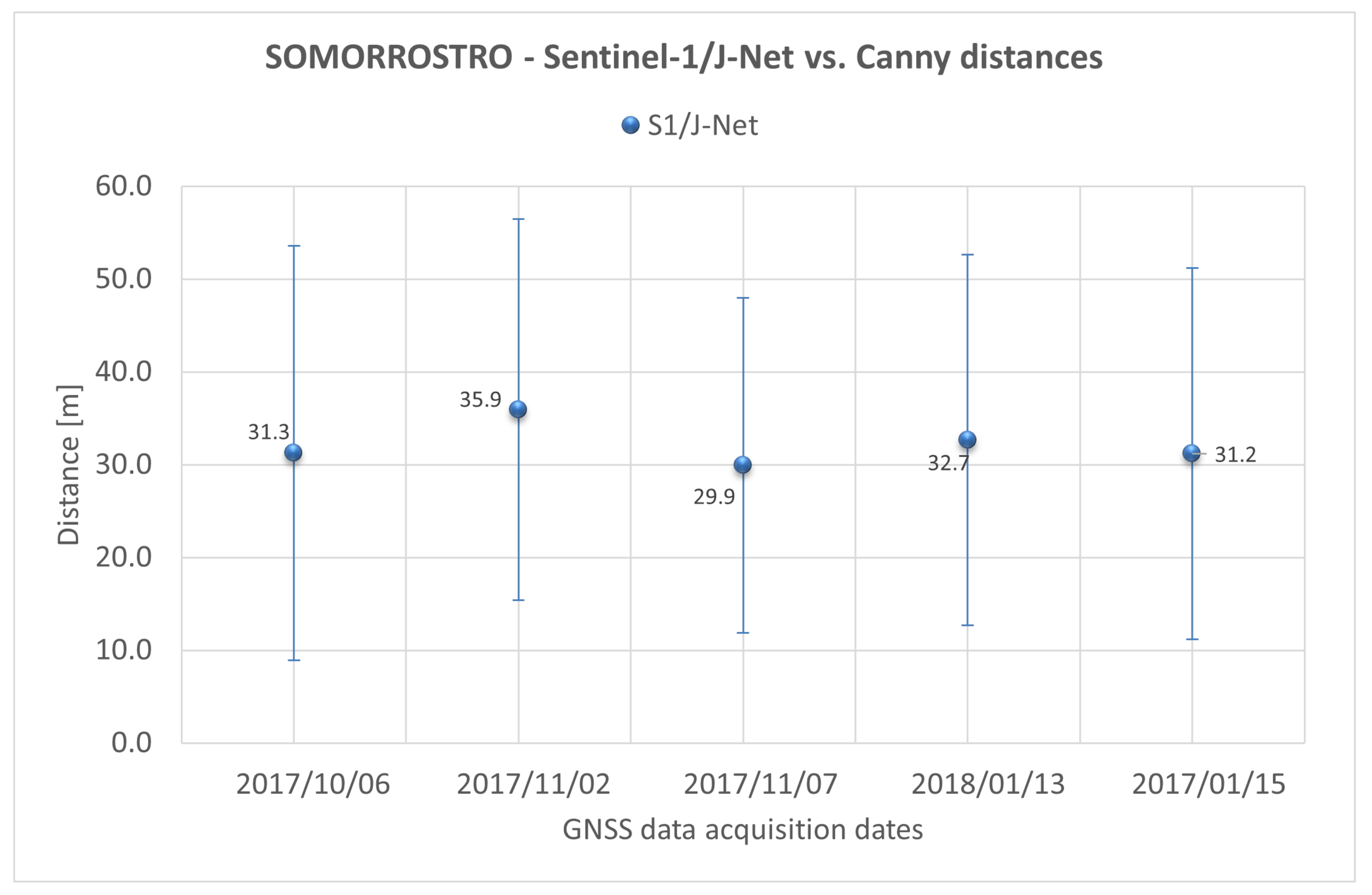
| 2017/10/04 | 2017/10/06 | 31.2 | 22.3 |
| 2017/11/03 | 2017/11/02 | 35.9 | 20.5 |
| 2017/11/09 | 2017/11/07 | 29.9 | 18.0 |
| 2017/11/15 | 2017/11/13 | 32.7 | 19.9 |
| 2017/11/15 | 2017/11/15 | 31.1 | 20.0 |
| Sentinel-2/Canny | |||
|---|---|---|---|
| Image | GNSS Reference | Mean (m) | Standard deviation (m) |
| Castelldefels Beach | |||
| 2017/06/02 | 2017/05/31 | 3.2 | 2.6 |
| 2017/11/19 | 2017/11/20 | 5.2 | 3.1 |
| 2017/11/19 | 2017/11/23 | 5.3 | 3.2 |
| 2018/01/18 | 2018/01/17 | 12.7 | 2.9 |
| 2018/01/18 | 2018/01/18 | 10.3 | 3.1 |
| 2018/03/14 | 2018/03/14 | 10.6 | 2.8 |
| Somorrostro Beach | |||
| 2017/10/10 | 2017/10/06 | 5.2 | 2.6 |
| 2017/10/30 | 2017/11/02 | - | - |
| 2017/11/09 | 2017/11/07 | 12.6 | 4.9 |
| 2017/11/14 | 2017/11/13 | 12.2 | 5.4 |
| 2017/11/14 | 2017/11/15 | 14.1 | 5.9 |
| Sentinel-1/Canny | |||
|---|---|---|---|
| Image | GNSS Reference | Mean (m) | Standard deviation (m) |
| Castelldefels Beach | |||
| 2017/05/31 | 2017/05/31 | 24.4 | 9.9 |
| 2017/11/21 | 2017/11/20 | 7.5 | 5.0 |
| 2017/11/21 | 2017/11/23 | 8.2 | 5.9 |
| 2018/01/20 | 2018/01/17 | 25.4 | 9.6 |
| 2018/01/20 | 2018/01/18 | 24.3 | 10.6 |
| 2018/03/15 | 2018/03/14 | 24.0 | 12.1 |
| Somorrostro Beach | |||
| 2017/10/04 | 2017/10/06 | - | - |
| 2017/11/03 | 2017/11/02 | - | - |
| 2017/11/09 | 2017/11/07 | - | - |
| 2017/11/15 | 2017/11/13 | - | - |
| 2017/11/15 | 2017/11/15 | - | - |
| Sentinel-2/CoastSat | |||||
|---|---|---|---|---|---|
| Image | GNSS Reference | Mean (m) | St. Dev. (m) | Mean (m) | St. Dev. (m) |
| Auto Threshold | Manual Threshold | ||||
| Castelldefels Beach | |||||
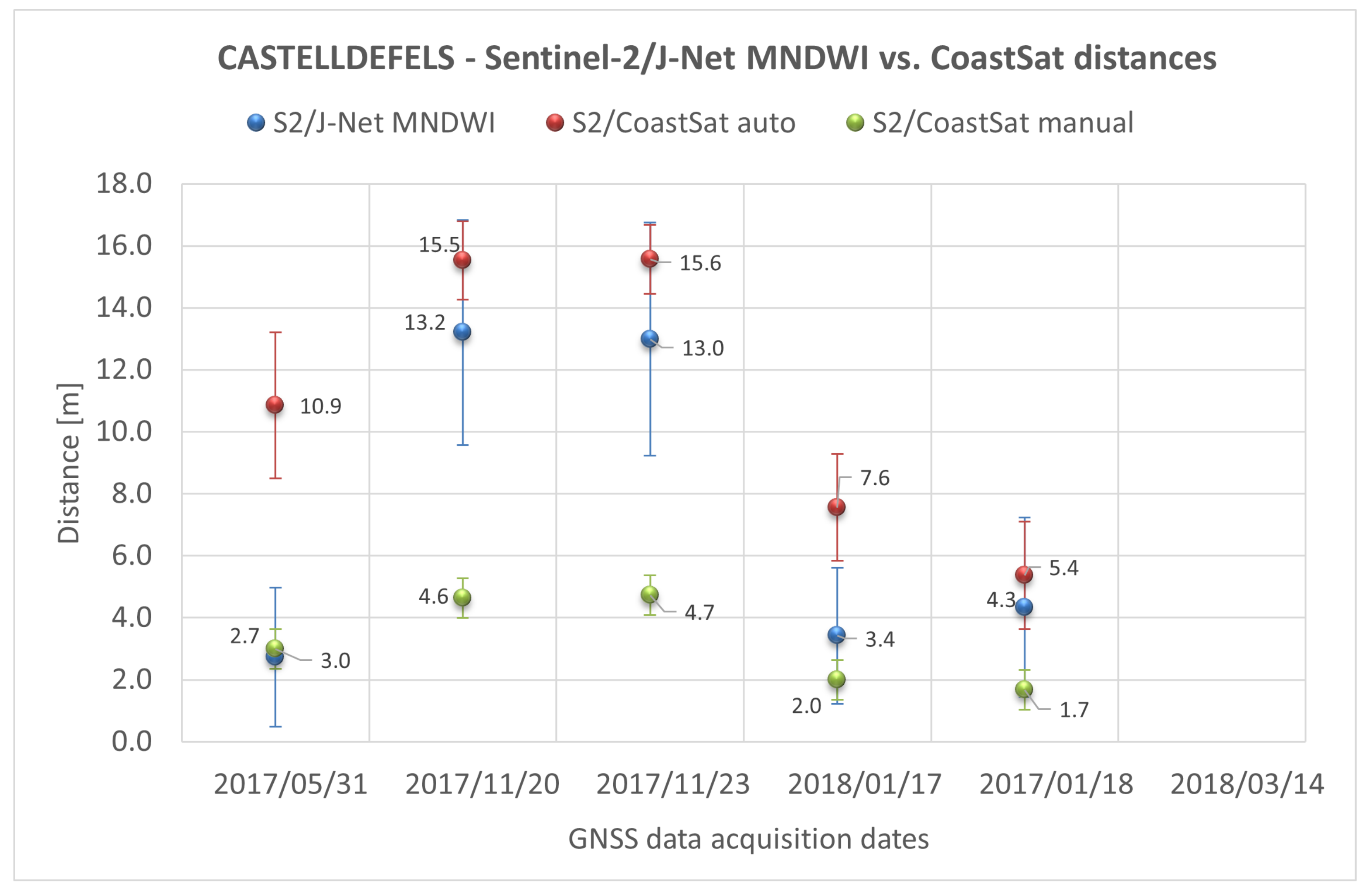
| 2017/06/02 | 2017/05/31 | 10.9 | 2.4 | 3.0 | 1.6 |
| 2017/11/19 | 2017/11/20 | 15.5 | 1.3 | 4.6 | 2.0 |
| 2017/11/19 | 2017/11/23 | 15.6 | 1.1 | 4.7 | 1.9 |
| 2018/01/18 | 2018/01/17 | 7.6 | 1.7 | 2.0 | 1.1 |
| 2018/01/18 | 2018/01/18 | 5.4 | 1.8 | 1.7 | 1.0 |
| Somorrostro Beach | |||||
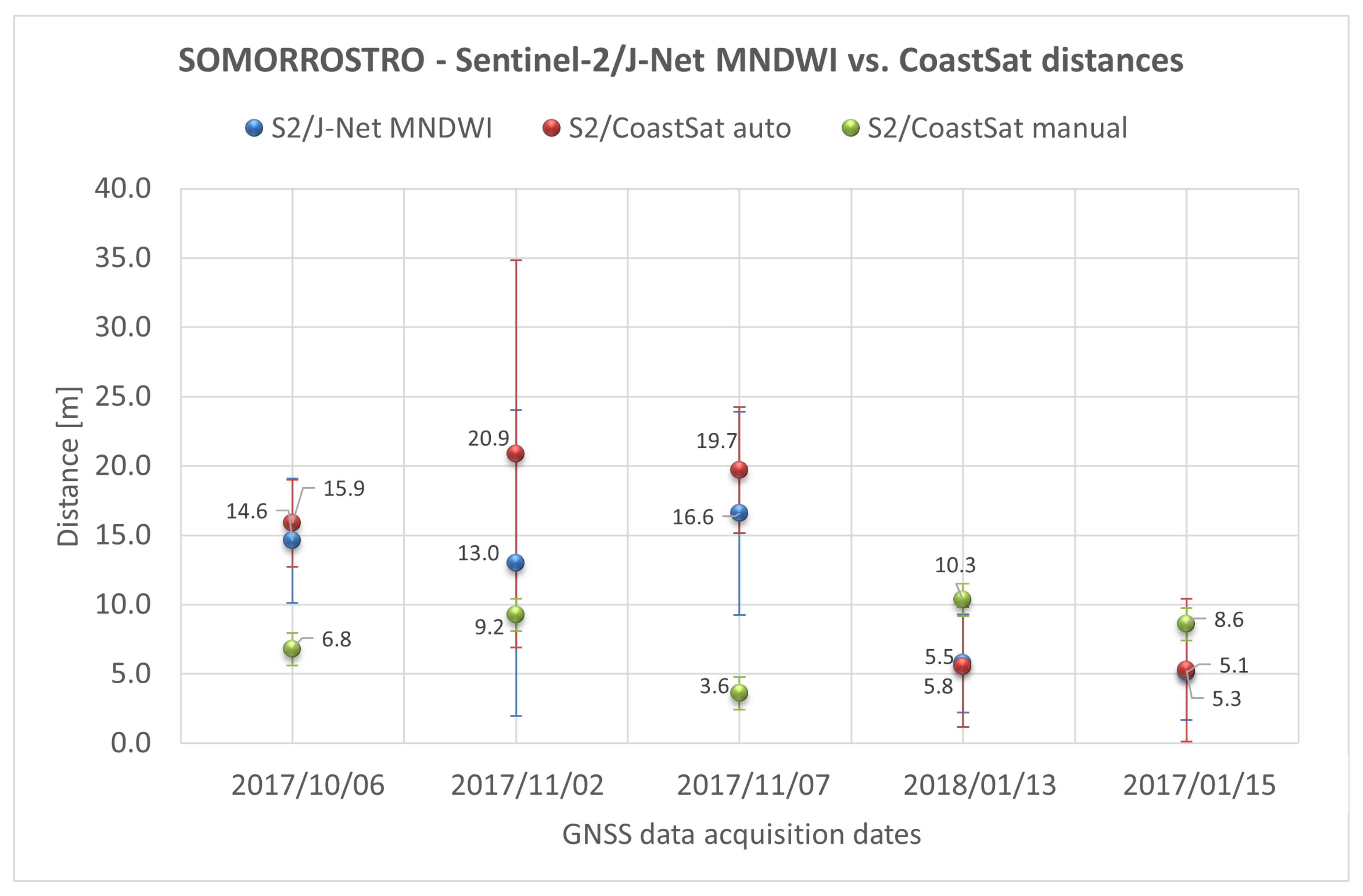
| 2017/10/10 | 2017/10/06 | 15.9 | 3.1 | 6.8 | 3.6 |
| 2017/10/30 | 2017/11/02 | 20.8 | 14.0 | 9.2 | 7.8 |
| 2017/11/09 | 2017/11/07 | 19.7 | 4.5 | 3.6 | 3.3 |
| 2017/11/14 | 2017/11/13 | 5.5 | 4.3 | 10.3 | 3.9 |
| 2017/11/14 | 2017/11/15 | 5.3 | 5.2 | 8.6 | 3.8 |
| Sentinel-2/MNDWI Plus J-Net Dynamic | |||
|---|---|---|---|
| Image | GNSS Reference | Mean (m) | Standard deviation (m) |
| Castelldefels Beach | |||
| 2017/06/02 | 2017/05/31 | 2.7 | 2.3 |
| 2017/11/19 | 2017/11/20 | 13.2 | 3.6 |
| 2017/11/19 | 2017/11/23 | 13.0 | 3.8 |
| 2018/01/18 | 2018/01/17 | 3.4 | 2.2 |
| 2018/01/18 | 2018/01/18 | 4.3 | 2.9 |
| Somorrostro Beach | |||
| 2017/10/10 | 2017/10/06 | 14.6 | 4.5 |
| 2017/10/30 | 2017/11/02 | 13.0 | 11.0 |
| 2017/11/09 | 2017/11/07 | 16.6 | 7.3 |
| 2017/11/14 | 2017/11/13 | 5.8 | 3.5 |
| 2017/11/14 | 2017/11/15 | 5.1 | 3.4 |
| Image Date | GNSS Date | Gap (d) | z (m) | H (m) | E (mh) | x (m) |
|---|---|---|---|---|---|---|
| Castelldefels Beach S2 | ||||||
| 2017/06/02 | 2017/05/31 | 2.1 | 0.05 | 0.05 | 8.1 | −0.2 |
| 2017/11/19 | 2017/11/20 | 1 | −0.01 | 0.01 | 5 | 0.4 |
| 2017/11/19 | 2017/11/23 | 4.2 | 0.01 | 0.15 | 12.4 | −1.8 |
| 2018/01/18 | 2018/01/17 | 0.8 | −0.03 | 0.09 | 22.1 | 0 |
| 2018/01/18 | 2018/01/18 | 0.1 | 0.02 | 0.13 | 1.9 | 0 |
| 2018/03/14 | 2018/03/14 | 0.1 | 0.05 | 0 | 0.5 | 0 |
| Castelldefels Beach S1 | ||||||
| 2017/05/31 | 2017/05/31 | 0.1 | −0.03 | −0.02 | 1.3 | 0 |
| 2017/11/21 | 2017/11/20 | 1 | −0.03 | 0.04 | 3.5 | −0.4 |
| 2017/11/21 | 2017/11/23 | 2.2 | −0.01 | 0.18 | 4.2 | −2.6 |
| 2018/01/20 | 2018/01/17 | 2.8 | −0.09 | 0.45 | 31.5 | −7.6 |
| 2018/01/20 | 2018/01/18 | 2.1 | −0.04 | 0.49 | 11.4 | −5.5 |
| 2018/03/15 | 2018/03/14 | 1.1 | −0.09 | −0.6 | 15.7 | 4.4 |
| Somorrostro Beach S2 | ||||||
| 2017/10/10 | 2017/10/06 | 4.1 | −0.15 | 0.2 | 60.9 | - |
| 2017/10/30 | 2017/11/02 | 2.9 | 0.05 | 0.02 | 39.4 | - |
| 2017/11/09 | 2017/11/07 | 2.1 | 0.06 | 0.24 | 42 | - |
| 2017/11/14 | 2017/11/13 | 1.1 | −0.15 | −0.14 | 36.4 | - |
| 2017/11/14 | 2017/11/15 | 1.1 | 0.02 | −0.31 | 54.1 | - |
| Somorrostro Beach S1 | ||||||
| 2017/10/04 | 2017/10/06 | 1.9 | 0.09 | −0.1 | 13.5 | - |
| 2017/11/03 | 2017/11/02 | 1.1 | 0 | 0.28 | 4.8 | - |
| 2017/11/09 | 2017/11/07 | 2.1 | 0.06 | 0.24 | 42 | - |
| 2017/11/15 | 2017/11/13 | 2.1 | −0.15 | 0.07 | 85.3 | - |
| 2017/11/15 | 2017/11/15 | 0.1 | −0.02 | 0.09 | 4.4 | - |
Disclaimer/Publisher’s Note: The statements, opinions and data contained in all publications are solely those of the individual author(s) and contributor(s) and not of MDPI and/or the editor(s). MDPI and/or the editor(s) disclaim responsibility for any injury to people or property resulting from any ideas, methods, instructions or products referred to in the content. |
© 2023 by the authors. Licensee MDPI, Basel, Switzerland. This article is an open access article distributed under the terms and conditions of the Creative Commons Attribution (CC BY) license (https://creativecommons.org/licenses/by/4.0/).
Share and Cite
Zollini, S.; Dominici, D.; Alicandro, M.; Cuevas-González, M.; Angelats, E.; Ribas, F.; Simarro, G. New Methodology for Shoreline Extraction Using Optical and Radar (SAR) Satellite Imagery. J. Mar. Sci. Eng. 2023, 11, 627. https://doi.org/10.3390/jmse11030627
Zollini S, Dominici D, Alicandro M, Cuevas-González M, Angelats E, Ribas F, Simarro G. New Methodology for Shoreline Extraction Using Optical and Radar (SAR) Satellite Imagery. Journal of Marine Science and Engineering. 2023; 11(3):627. https://doi.org/10.3390/jmse11030627
Chicago/Turabian StyleZollini, Sara, Donatella Dominici, Maria Alicandro, María Cuevas-González, Eduard Angelats, Francesca Ribas, and Gonzalo Simarro. 2023. "New Methodology for Shoreline Extraction Using Optical and Radar (SAR) Satellite Imagery" Journal of Marine Science and Engineering 11, no. 3: 627. https://doi.org/10.3390/jmse11030627