
A Theory of Orbital-Forced Glacial Cycles: Resolving Pleistocene Puzzles

Lamont–Doherty Earth Observatory, Columbia University, Palisades, NY 10964, USA
†
Retired.
J. Mar. Sci. Eng. 2023, 11(3), 564; https://doi.org/10.3390/jmse11030564
Submission received: 9 January 2023
/
Revised: 3 March 2023
/
Accepted: 3 March 2023
/
Published: 6 March 2023
(This article belongs to the Special Issue Oceanic and Marine Circulation: Numerical Modelling and Analysis of Observations)
Abstract
:It is recognized that orbital forcing of the ice sheet is through the summer air temperature, which however covaries with the sea surface temperature and both precede the ice volume signal, suggesting the ocean as an intermediary of the glacial cycles. To elucidate the ocean role, I present here a minimal box model, which entails two key physics overlooked by most climate models. First, I discern a robust ‘convective’ bound on the ocean cooling in a coupled ocean/atmosphere, and second, because of their inherent turbulence, I posit that the climate is a macroscopic manifestation of a nonequilibrium thermodynamic system. As their deductive outcome, the ocean entails bistable equilibria of maximum entropy production, which would translate to bistable ice states of polar cap and Laurentide ice sheet, enabling large ice-volume signal when subjected to modulated forcing. Since the bistable interval is lowered during Pleistocene cooling, I show that its interplay with the ice–albedo feedback may account for the mid-Pleistocene transition from 41-ky obliquity cycles to 100-ky ice-age cycles paced by eccentricity. Observational tests of the theory and its parsimony in resolving myriad glacial puzzles suggest that the theory has captured the governing physics of the Pleistocene glacial cycles.
1. Introduction
In late Pleistocene, the global ice volume exhibits pronounced variation at orbital periods [1]. As Antarctica has reglaciated since late Miocene [2], the ice-volume signal reflects mainly that of the northern ice sheet, whose correlation with the Milankovitch insolation (MI, all acronyms are listed in Abbreviations) supports the astronomical theory that it is the summer surface air temperature (SAT) that controls the ice margin [3]. The orbital forcing of the SAT however cannot be direct since the atmosphere is mainly heated from below and although its absorption of the SW flux dominates the summer heating [4], the summer SAT is still largely bounded by the underlying sea surface temperature (SST) to maintain the radiative–convective equilibrium that defines the troposphere, a feature that is indeed seen distinctively in their global distribution [5] (their figure 10.7, lower panel). Because of this ‘convective bound’, the annual SAT registered in the ice core data covaries strongly with the SST through glacial cycles, which are synchronous in both hemispheres [6,7,8] and lead the global ice volume by about two millennia [1,9,10]. This observation suggests that the ocean must be an intermediary of the orbital forcing of the ice sheet, as is also strongly argued by [11] but unfortunately is often overlooked. Given the causative role of the SST in regulating the summer SAT, hence the ice margin, its reproduction by numerical models should be a prerequisite for a prognostic simulation of the glacial cycles—a benchmark not yet met, which also calls into question the wide-spread practice of parameterizing the SAT in terms of the solar insolation but applying slab, mixed-layer, or diffusive ocean models [12,13,14,15].
The SST is regulated by the meridional overturning circulation (MOC), which is comprised partly of random eddy exchange across the subtropical front [16,17]. For primitive-equation models that do not resolve eddies, the MOC takes the form of a laminar overturning cell whose strength depends critically on the diapycnal diffusivity [18], which is in effect a free parameter finely tuned to yield the observed state [19]. To prognose MOC variability from primitive equation models [20], there seems to be no substitute than resolving eddies, which remains prohibitive because of the long integration needed to simulate glacial cycles (see further discussion in Section 5). A theoretical construct, however, is free from such restraint and, applying a probability law of the nonequilibrium thermodynamics (NT), I have previously deduced that the MOC would self-propel on millennial timescale toward maximum entropy production (MEP), which may replicate the current climate without tuning [21]. In this paper, I shall show that the interplay of this ‘MEP adjustment’ with orbital forcing and ice–albedo feedback may provide a robust explanation of the Pleistocene glacial cycles while resolving many longstanding puzzles.
One such puzzle is the mid-Pleistocene transition (MPT) from 41- to 100-ky cycles when there is no appreciable change in MI [22,23]. Although early focus was on the genesis of the 100-ky cycles, not to be overlooked is their absence in early Pleistocene, which would weed out some resolutions of the ‘100-ky problem’. These include internal ice sheet oscillations [24,25,26,27] and stochastic dynamics [28,29,30] since these mechanisms should be operative in early Pleistocene when the northern hemisphere glaciation has already set in [31] and yet there are no 100-ky cycles. Then there are conceptual and dynamic-system models tuned to match observed glacial cycles [32,33,34,35,36,37], but since some key parameters do not correspond to measurable quantities hence are unconstrained, these models are mostly unfalsifiable to constitute testable physical theories.
A plausible and well-explored paradigm of the glacial cycles is that the ice sheet is bistable, so eccentricity can generate 100-ky cycles through its modulation of the forcing amplitude, and if the hysteresis thresholds were lowered by putative decrease of pCO2 or regolith removal during Pleistocene, one could have a plausible account of MPT [14,23,38]. However, there is little evidence of pCO2 trend through MPT [39] and regolith change is poorly constrained by observation, rendering their timing of the MPT uncertain. Even more problematic, the postulated ice bistability involves ice-free state [40,41], which cannot characterize the interglacial, as attested by the present Greenland ice sheet, and if such ice-free state were realized in early Pleistocene, the ice volume signal would be minimal [42], hence at odds with the pronounced 41-ky cycles observed [43]. To preserve the hysteresis paradigm, one therefore needs to invoke different bistability, which, as we shall see, can be engendered by the ocean.
Since the main difference of our theory is an eddying ocean filtering the orbital forcing of the ice margin, I shall formulate a minimal box model to isolate this physics. In the following, I elucidate first the inner working of our coupled climate system in Section 2 and then discuss how the ocean may filter the orbital forcing to generate glacial cycles in Section 3. I highlight how the theory may resolve prevailing Pleistocene puzzles in Section 4 and provide additional discussion in Section 5 to conclude the paper.
2. Coupled Climate Model
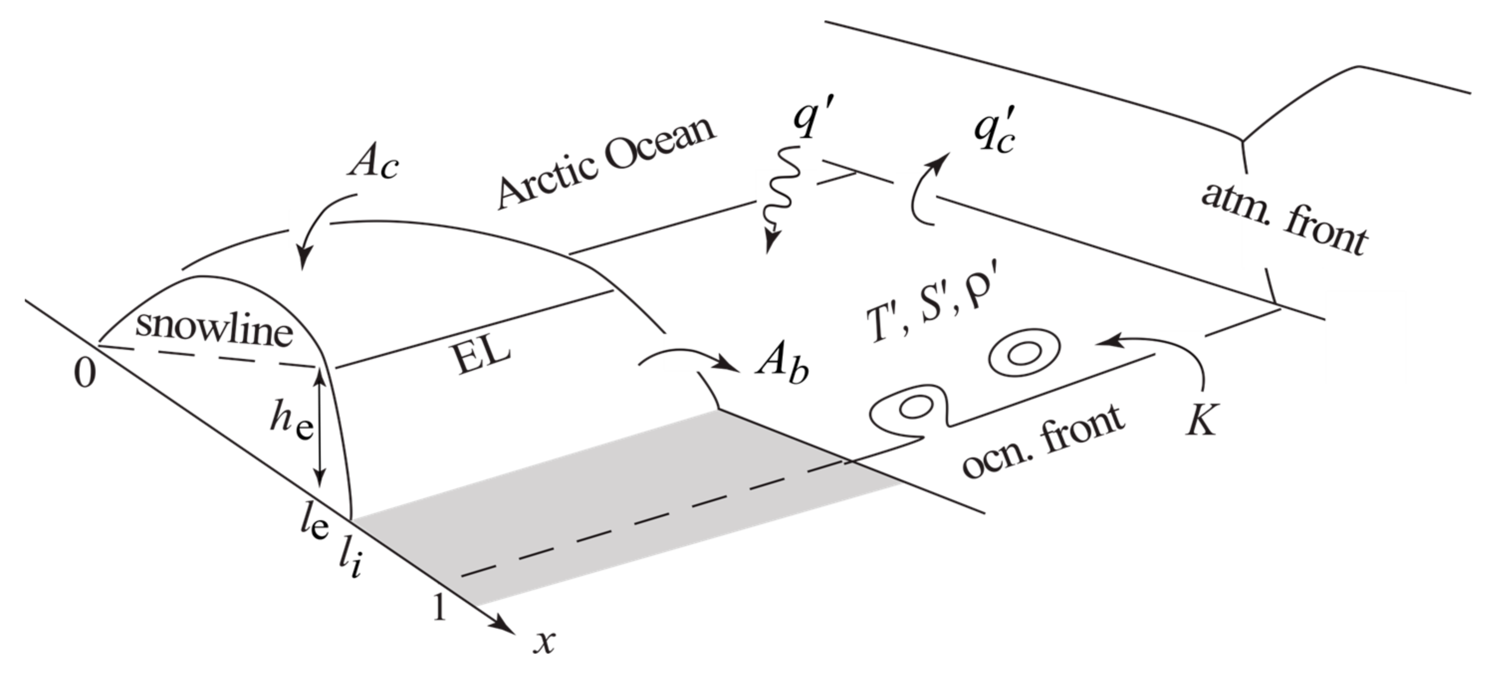
The model configuration sketched in Figure 1 pertains to the North Atlantic where glacial cycles are more sharply defined. Both ocean and atmosphere are divided into warm/cold masses by mid-latitude fronts—a discernible first-order description of the observed state, and ice sheets may form on continents terminating at an ice-covered Arctic Ocean. Since both forcing and response of the glacial cycles are dominated by that of the cold boxes, the model variables are the cold-box deviations (primed) from global means (overbarred, assumed known), which are nondimensionalized by scales (bracketed) listed in Appendix A, the latter also contains all symbols and parameters used in the model. Given the small range of the SST relative to its global mean (in absolute unit), we neglect for simplicity latitudinal variation of the outgoing and surface long-wave (LW) fluxes compared with the absorbed short-wave (SW) and convective fluxes (both are twofold greater), and given the large thermal inertia of the ocean, we neglect its seasonality [44] (their figure 15). Retaining dominant balances therefore, the external forcing is the cold-box deficit of the annual absorbed SW flux (), which would induce a deficit in the SST (), hence the convective flux (). The accompanying atmospheric heat hence moisture transport would induce a salinity deficit (), which counters the temperature deficit in the manifested density surplus (). The latter drives the MOC (of strength K) across the subtropical front, which is composed partly of random eddies. For the ice sheet, the total ablation () and accumulation (), both are prognostic, would constrain the equilibrium line (EL) altitude (ELA, ), hence its x-coordinate () as well as the ice margin ().
2.1. Regime Diagram
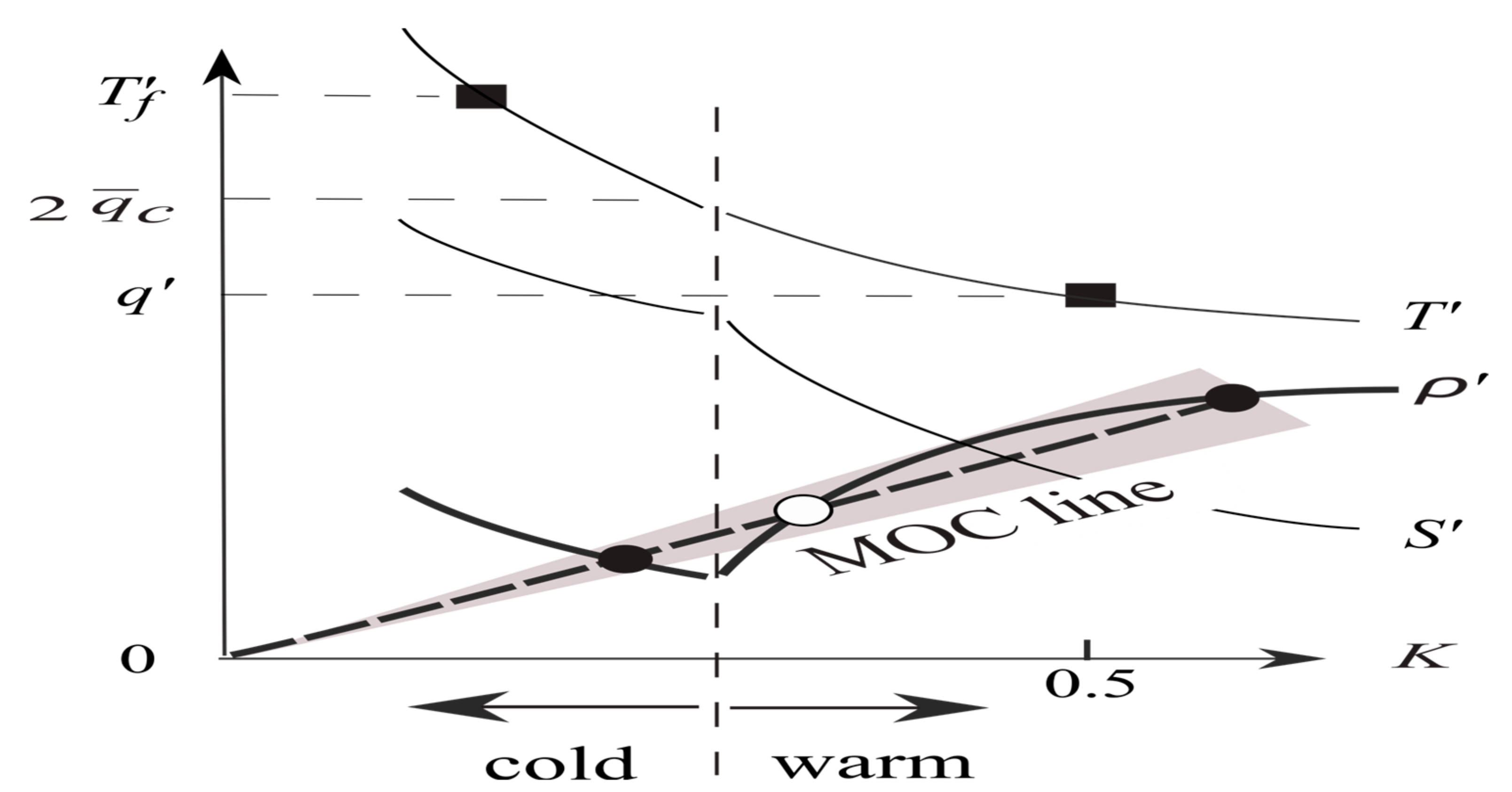
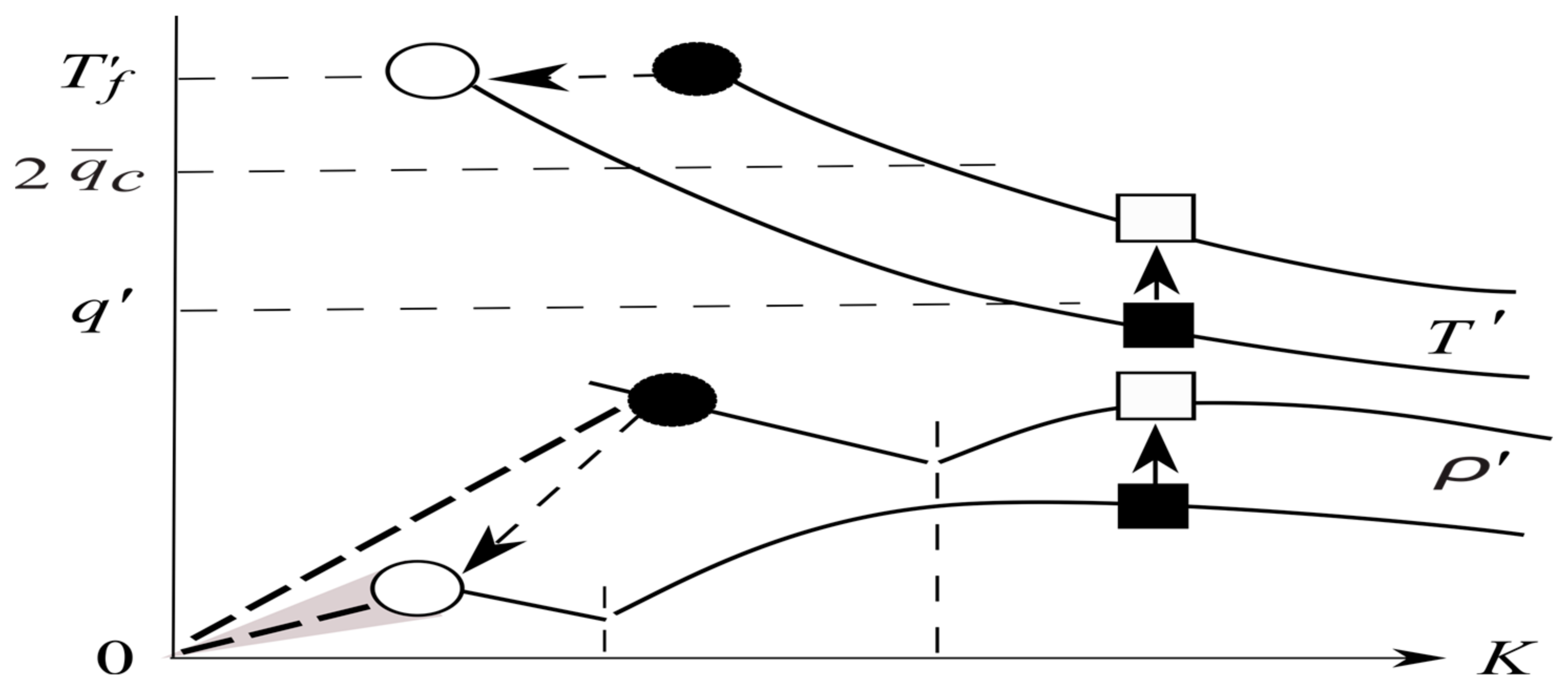
Readers are referred to [21] for detailed mathematical derivation of our climate model, but the following discussion should suffice in elucidating the model physics. For this purpose, I draw in Figure 2 a ‘regime diagram’ spanned by the (nondimensionalized) MOC (abscissa) and density surplus (ordinate, markings pertain to the temperature deficit), so a climate state is specified by the intersect of two lines: the ‘density line’ (thick solid)—an outcome of the thermohaline balances of the ocean, and the ‘MOC line’ (thick dashed) encoding the MOC dependence on the density surplus, as discussed sequentially below.
The density surplus line represents the spacing between temperature and salinity deficit lines (thin solid), whose dependence on the MOC is readily discerned from the thermohaline balance of the ocean. Decreasing the MOC, for example, would cool the subpolar water (that is, raise the temperature line), which would reduce the convective flux (not shown) to augment the atmospheric heat transport. The latter in turn would moderate the ocean cooling in reducing the slope of the temperature line. There is, however, a limit to such moderation since the convective flux may not be negative, and with its deficit () from the global mean () being /2 (the factor 2 stemming from concurrent cooling of the surface air [21]), we deduce a ‘convective bound’ at:
as indicated by the vertical dashed line, which would divide the climate regime into warm/cold branches. In the cold branch, the convective flux is nil, so the atmospheric heat transport has saturated at to no longer moderate the ocean cooling, resulting in a steeper temperature line.
Since the atmospheric heat transport also transports moisture, it freshens the subpolar water, more so when the MOC weakens as seen in the rising salinity line. In the warm branch, the salinity line, being compounded by the increasing moisture transport, is steeper than the temperature line. In the cold branch, however, the moisture transport has saturated with the atmospheric heat transport, so the salinity deficit increases at the same rate as the temperature deficit (inverse in the MOC). Since the density surplus is the difference of the two, the density line exhibits a break in its slope at the convective bound so that it may remain positive in the cold branch. This feature, being a consequence of the ocean/atmosphere coupling via the convective bound, is absent from ocean-only models [45] for which the density line would continue its downward trend as the MOC decreases to become negative, a state unrealized in the North Atlantic.
The density line constitutes a climate continuum and an additional constraint on the MOC is needed to specify the climate state. For simplicity, I assume the MOC to be linear in the density surplus [46] with the proportional constant coined ‘admittance’ (drawing its analogy in electrostatics with density/MOC playing the role of voltage/current), whose inverse sets the slope of the MOC line. In primitive equation models that do not resolve eddies, the MOC takes the form of a laminar overturning cell, and the admittance is encapsulated by the diapycnal diffusivity, which in effect is a free parameter finely tuned to yield the observed state. For the example shown in Figure 2, the ocean is bistable and the two equilibria (solid ovals, the open oval being an unrealized saddle point) are those uncovered by [47] in a coupled model and, in support of our convective bound, their cold state is indeed characterized by a vanishing convective flux [47] (their figure 18).
In the actual ocean, on the other hand, the admittance is not a free parameter but subjected to microscopic fluctuations associated with random eddy exchange across the subtropical front. Applying the fluctuation theorem (FT), a generalized second law [48], ref. [21] deduces that the admittance would self-propel on millennial timescale toward MEP, a tendency termed ‘MEP adjustment’. Although the veracity of MEP remains debated, it has gained growing acceptance among climate theorists [49,50,51] and if, as contended by [21], it is a deductive outcome of FT—the latter being of considerable mathematical rigor and has been tested in a laboratory setting [52,53], it would further strengthen the physical basis of MEP. In addition, a recent direct numerical simulation (DNS) of horizonal convection has produced a mid-latitude front [54], a feature that is absent from laminar models [55] but is just as predicted by MEP [56] to offer a palpable computational support. As a further demonstration of its utility, ref. [57] has recently shown that MEP adjustment may provide an integrated account of abrupt climate changes of the late Pleistocene. With the above, I am justified to pose MEP adjustment as a working hypothesis in the closure of our theory. To aid the visualization, I have blurred the MOC line in Figure 2 to signify microscopic fluctuations, whose probability bias in accordance with FT would pivot the MOC line over millennial timescale toward MEP, the latter are as marked by rectangles and discussed in the next section.
To recap, I have argued that since the convective flux may not be negative in a coupled ocean/atmosphere, there is a limit to the cooling of the subpolar ocean, giving rise to a robust convective bound that divides warm/cold climate regimes. The latter may account for the bistable ocean states uncovered in coupled models, which thus provides a computational support of the convective bound.
2.2. MEP States
For a quasi-steady state ocean, the irreversible entropy production equals the entropy flux exiting its upper surface [51,56], locally a division of the heat flux by the SST (in absolute unit). Given the small SST variation and the box approximation, the global entropy flux is further reduced to a product of the ocean heat transport () and the differential temperature . One readily sees from Figure 2 that this product could have a local maximum in the warm branch, which is derived to be:
and will be referred as the warm MEP. The cold box SST thus varies linearly with the forcing or dimensionally (starred) , where is the relatively well-constrained air–sea transfer coefficient. Setting °C−1 [21], an absorbed SW flux 100 below the global mean would induce a subpolar water 8 °C cooler than the global mean, not unlike the current interglacial [44] (their figure 15). Somewhat surprising, the MOC in (2) is unaffected by forcing, which can be attributed to the latter’s buffering by the thermal response. In fact, from its scaling definition, we see that the MOC is a function only of the air–sea transfer coefficient to yield a transport of 14 Sv (for a basin width of ), which is commensurate with the observed one [58]. Since our MOC contains no free parameter, this observational test is more stringent than that involving tunned diapycnal diffusivity [18].
For the cold branch, the atmospheric heat transport has saturated, so has the ocean heat transport—for a given forcing. As such, the entropy production increases unabated with until the subpolar water is cooled to the freezing point:
that is nonetheless free of the perennial ice, which will be referred as the cold MEP. The freezing-point coldness is consistent with that seen in the last glacial maximum (LGM) [44] (their figure 15), and the absence of the perennial ice is because such ice would cut down the ocean cooling to weaken the ocean heat transport, contradicting the MEP. It should be noted, however, that since MEP adjustment occurs over millennial timescale, such ice-free ocean does not preclude sea ice formation over shorter timescales, including the seasonal one. In fact, with the subpolar water hovering around the freezing point during the LGM, extensive sea ice necessarily forms in winter, as is the observed case, but tellingly the subpolar ocean remains largely open in summer [59] (their figure 10, upper-left panel), which may be explained by the MEP. The absence of the summer sea ice incidentally downgrades its role in limiting the moisture source hence in regulating the glacial cycles [60]. With the fixed temperature no longer buffering the orbital forcing, the MOC of the cold MEP is variable, which nonetheless is quite a bit weaker than that of the warm MEP, as seen in observations [61,62].
To recap, I have identified MEPs in both warm/cold branches: the warm MEP being characterized by subpolar SST proportional to the forcing and a MOC that depends only on the air/sea transfer coefficient, and the cold MEP by the freezing-point subpolar water that is nonetheless free of the perennial ice. Their distinctions comport with observed glacial/interglacial (G/IG) oceans to support the latter’s interpretation as MEP states. I shall now apply our climate model in an expanded theoretical framework to examine the glacial cycles, the object of the present study.
3. Glacial Cycles
3.1. Orbital Forcing
With the ocean being the primary entry point of the orbital forcing into the climate system and the neglect of the seasonal SST, the relevant forcing of the glacial cycles is the annual absorbed SW flux. At orbital periods, this forcing is dominated by that over the high latitudes, being an order of magnitude greater than that over the tropics [63] (their figure 2.7), and then over the high latitudes, it is dominated by that of the summer due to both the vanishing, hence unvarying, winter insolation [64] (his figure 18b) and the ice–albedo feedback that preferentially depresses the forcing trough. These are general properties of both obliquity and precession forcings, whose latitudinal difference [65] is also somewhat allayed by spatial averaging over the subpolar ocean. This insensitivity to the forcing partition is incidentally consistent with model calculations [41].
This commonality notwithstanding, we must recognize the critical importance of the ice–albedo feedback in instituting the precession forcing, which otherwise would be nil because of the Kepler’s second law. This constraint is often overlooked and cannot be bypassed by positing an ablation dependence on insolation [66]—as it would conflict with the dominant ablation control by the summer SAT [67]. Since our forcing is the annual absorbed SW flux, the above Kepler’s stricture is naturally removed by the activation of the ice–albedo feedback as Pleistocene cools, and since the albedo increase during glacial period can be inferred from observation, its effect on the forcing can be quantified, as estimated next.
Based on [68], I take the G/IG ice cover difference to be half the subpolar area and assume ice/land albedo difference of 0.6, then the albedo increase that depresses the glacial summer insolation is 0.3. Setting MI range of [450,500] [69] and a planetary albedo and atmospheric attenuation of 0.3, the absorbed SW flux would have a range of 0. in summer, which would be halved to 83 for the annual mean. As this is of the same order of magnitude as the MI range, I shall take MI as a convenient proxy for late Pleistocene forcing. I should stress that our use of MI is not because of its direct effect on the summer SAT, as erroneously applied previously [66,70], but because it mimics the annual absorbed SW flux that drives the SST, which anchors the summer SAT.
To recap, since the relevant forcing of the ocean is the annual absorbed SW flux regulable by ice albedo, it entails little precession signal in the warm early Pleistocene because of Kepler’s second law but mimics the MI in late Pleistocene when the ice–albedo feedback is activated by the Pleistocene cooling.
3.2. Hysteresis
It is readily seen from Figure 2 that subjected to freshwater perturbation that moves the density line up and down, the ocean may exhibit hysteresis between warm and cold branches, a topic widely explored previously [19,21]. Such short-term hysteresis, however, has no import on the orbital-induced hysteresis between warm/cold MEPs propelled by the pivoting MOC line, as illustrated in the regime diagram shown below (Figure 3).
Suppose one is at the warm MEP of fixed MOC (rectangles), lowering the summer insolation would cool and densify the subpolar water (that is, raising both temperature and density lines) to move the warm MEP upward (the solid arrows from solid to open rectangles), and when the temperature deficit exceeds the convective bound (), there is no longer warm MEP and the ocean would enter the cold branch to be propelled toward the cold MEP (ovals). With (1) and (2), this cold transition occurs at:
a function only of the global convective flux, an external parameter.
Now suppose one is at the cold MEP of freezing point SST (ovals), then raising the summer insolation would warm and lighten the subpolar water (that is, lower the temperature and density lines) to move the cold MEP as indicated by the dashed arrows from solid to open ovals. The flattened MOC line (thick dashed) compounded by microscopic fluctuations (shaded cone) may no longer intersect the density line in the cold branch, thus propelling the ocean into the warm branch. As a conservative upper bound of the warm transition, one may set it to when the MOC line is level to yield [21] (from his equations (8), (12) and (13) setting ):
where is a dimensionless moisture parameter with a value of about 0.3 [21] (his appendix D). The above two thresholds (4)–(5) define the ‘bistable interval’, which thus is a function only of the global convective flux, and if this bistable interval is traversed by the orbital forcing, there would be hysteresis between warm/cold MEPs of the ocean.
To recap, I show that the ocean may exhibit hysteresis between warm/cold MEPs when the orbital forcing traverses the bistable interval set by the global convective flux. The cold transition occurs when forcing-induced cooling exceeds the convective bound to vault the ocean into the cold branch, and the warm transition occurs when forcing-induced warming hence lightening the subpolar water may no longer contain the weak MOC, which would be reactivated to vault the ocean into the warm branch.
I shall next examine how the bistable MEP states of the ocean may translate to that of the ice margin, which anchors the glacial cycles.
3.3. Ice Margin
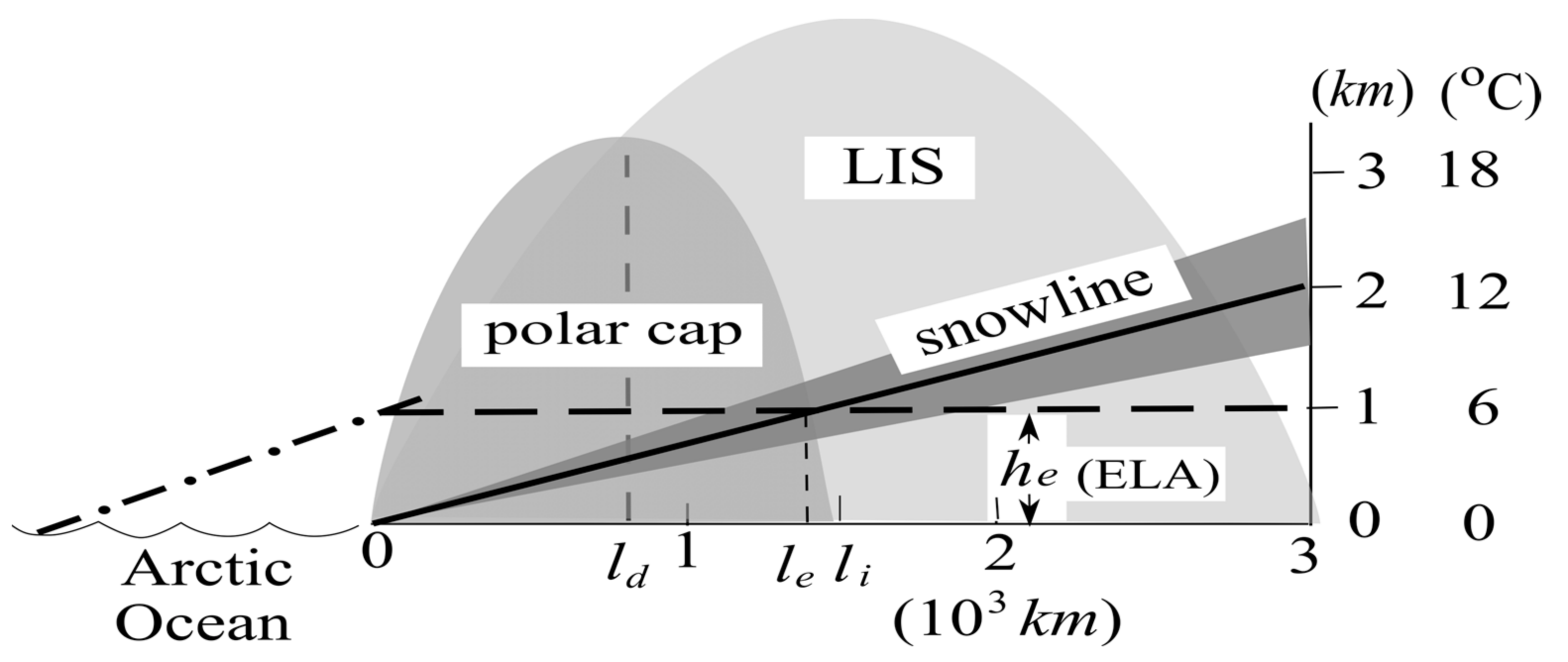
For simplicity, I take the southern margin of the continental ice sheet to be zonal [68], so it is regulated by the summer SAT of the adjacent ocean, which moreover is approximated by the underlying SST because of the convective bound (Section 1). To institute latitudinal temperature variation within the cold box needed for a variable ice margin, I assume that the SST is at the freezing point abutting the Arctic Ocean because of the perennial sea ice and that the ocean dynamics has smoothed its latitudinal gradient to render a linear profile, so it is as shown by the solid line in Figure 4 for the interglacial but flush with the x-axis for the glacial. The assumed SST profile and its alignment with the summer SAT are supported by observations [5] (their figure 7.5) [44] (their figure 15). Such spatial variation only slightly modifies the entropy production of the box model, so the earlier derivation of the MEP state remains valid. Setting a constant lapse rate of °C km−1, the solid line also represents the interglacial snowline whose height is as marked on the ordinate, and the glacial snowline is aligned with the x-axis. In the following derivation, variables are subscripted d, e and i, respectively, for ice ‘divide’, ‘equilibrium’ line, and ‘ice’ margin. The ice sheet would advance southward by accumulation until it is halted by increasing ablation, that is, when the snowline on its southern face attains the ELA to be derived below.
A prognosis of the ELA necessarily involves ice dynamics and mass balance. For minimal dynamics, I assume a plastic ice sheet of yield stress so the longitudinal momentum balance states [71]:
where h is the ice height and with , the gravitational acceleration and , the ice density. To check the adequacy of (6), an integration across half continental width (w) yields an ice divide height of:
and setting [72] and w = 500/1000 for Greenland/North America, the ice divide would stand at 3.3/4.6 km, commensurate with the present Greenland ice sheet and the Laurentide ice sheet (LIS) [68].
The yearly accumulation above the EL is dominated by the summer season because of the much colder, hence drier, winter air, and this accumulation is approximately the moisture transport crossing the EL since the moisture reaching beyond the ice divide is likely negligible [73] (his figure 10). As discussed in [74], the moisture transport (hence total accumulation ) can be linked to the atmospheric energy transport via:
where is now the summer energy transport into the polar cap (referring to the land ice in this paper) and the moisture parameter is defined by:
with being the water density, , the latent heat of sublimation and Bo, the ratio of sensible to latent heat transports. This ratio in turn varies with the surface temperature T as:
where is the saturation vapor pressure, a sharply decreasing function of cooling air on account of the Clausius–Clapeyron relation. Over the EL (of freezing-point temperature), Bo is about 5 [74] (his figure 4), so . If we set the summer energy transport into the latitude of the polar cap (say, 60° N) to be [5] (their figure 13.19), then, dividing by the length of the latitude circle, it yields , resulting in total accumulation of from (8). As a cursory check, for a distance of 500 km between EL and ice divide, the mean accumulation rate would be 0.19 , which is commensurate with the current Greenland ice sheet [75]. It is notable that the energy balance requirement and Clausius–Clapeyron relation have produced the observed accumulation regardless the vagaries of the atmospheric motion that carries the moisture [76]. On the other hand, although the total accumulation above the snowline is insulated from the surface climate, the local accumulation may vary strongly through the glacial cycles [77] due to the latitudinal movement of the snowline.
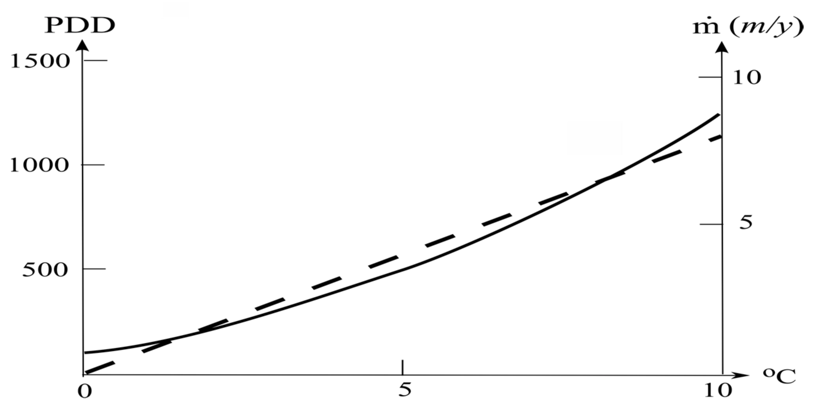
To prognose the ablation, I plot in Figure 5 (taken from [78], his figure 2) the positive degree day (PDD, the solid line) against July SAT for a seasonal amplitude of 10 °C representative of the high northern latitudes [5] (their figure 7.9). Applying a melt factor of 0.007 m per PDD [78], the melt rate is as marked on the right ordinate, which I approximate by the straight (dashed) line:
with my−1 °C−1. Integrating (11) over the ablation zone, we derive, using (6):
Equating ablation with the accumulation, we arrive at the ELA:
Applying the above estimate of accumulation yields hence an ice margin marked by sea level summer SAT of about 7 °C, both are commensurate with the present Greenland ice sheet [5] (their figure 7.4b), [79]. Pegging the ice margin by a specific summer isotherm has been used by [80], but their choice of 0 °C isotherm is deficient since there would be little summer ablation (Figure 5) to remove the yearly accumulation, and then it would yield an ice-free Greenland, contradicting the observed one. Although there are considerable uncertainties of the parameters entering (8) and (13), the sensitivity is dampened by the 1/3 power, so the deduced marking temperature of mid-single digits should generally apply. More significantly perhaps, this marking temperature is primarily an intrinsic property of the ice sheet, so the climate influence is relegated to moving the summer isotherms hence the temperature-tagged ice margin, as discussed next.
For the interglacial, the summer SAT is seen in Figure 4 to vary linearly with the forcing, but with the snowline pivoting about the Arctic rim, as indicated by the dark cone, there is always a polar cap (medium-shaded) whose southern margin thus moves with the forcing. For the glacial, on the other hand, the snowline is flush with the sea level in the subpolar zone, so the ice sheet would grow to the subtropical front corresponding to the LIS (light-shaded). Our model may thus explain the presence of Greenland ice sheet during the interglacial [6], the mid-latitude extent of the LIS [68], and why all ice ages seem to have comparable global ice volume [81].
Our bistable ice states differ fundamentally from that considered previously when the snowline, instead of pivoting about the Arctic rim, is displaced vertically [40,82], which would yield bistable equilibria of glacial polar cap and ice-free interglacial, the latter when the snowline no longer intersects the EL over land (the dash-dotted line). Since such a snowline intrudes deeply into the Arctic Ocean, it is predicated on an ice-free Arctic Ocean, a state not realized since about 5 million years ago (Ma) [83] hence cannot anchor their posited ice hysteresis.
To recap, I have derived a marking temperature of the ice margin as an intrinsic property of the ice dynamics, so bistable equilibria of the ocean would translate to that of the land ice of variable polar cap and a LIS extending to mid-latitudes, enabling large ice-volume signal during glacial cycles. Since glacial cycles exhibit qualitative transitions through the Pleistocene, any physical explanation of the glacial cycles must also account for such transitions, as discussed next.
3.4. Pleistocene Transitions
The MPT of glacial cycles from obliquity to eccentricity periods poses a significant challenge to the astronomical theory since MI displays no discernible change [14]. Unlike putative pCO2 decrease and regolith removal that are poorly constrained by observation (Section 1), there is pronounced Pleistocene cooling of more than 10 °C [31], a continuing trend of the tertiary [64] that is likely tectonic in origin and possibly involve several mechanisms [84,85]. Since tectonics is of multi-million to longer timescales, I shall take the Pleistocene cooling as external to the orbital forcing and examine its effect on glacial cycles.
I have shown earlier (Section 3.2) that the bistable interval is set by the global convective flux, and I shall next argue that this flux is lowered during Pleistocene cooling on account of the global ocean heat balance, which is of the form:
where , and are the global absorbed SW, convective and surface LW fluxes, respectively, and , the global ice cover. Pleistocene cooling would expand the ice cover and increase due to the drier air hence smaller downward LW flux, both thus reinforcing each other to reduce the global convective flux. Differentiating (14) with respect to the global SST, its rate of reduction is
for which I have set and assumed an ice surface expanding by 15% of the global area by 10 °C cooling [68] and a surface LW flux increasing by 3 per degree cooling [86] (his figure 1c). For 10 °C cooling, the global convective flux thus would decrease by 60 , which is quite substantial considering that it is only about 100 in the current interglacial. Although there is no proxy data for the convective flux, the inferred large decrease underscores its robustness, which certainly dwarfs the greenhouse effect of decreasing pCO2 (several [87]), so is the observed cooling compared with the pCO2-induced cooling of O (1 °C) [88] (their table 3). It is peculiar, therefore, that it is the greenhouse effect of pCO2 rather than the drying air that is commonly invoked to explain the MPT.
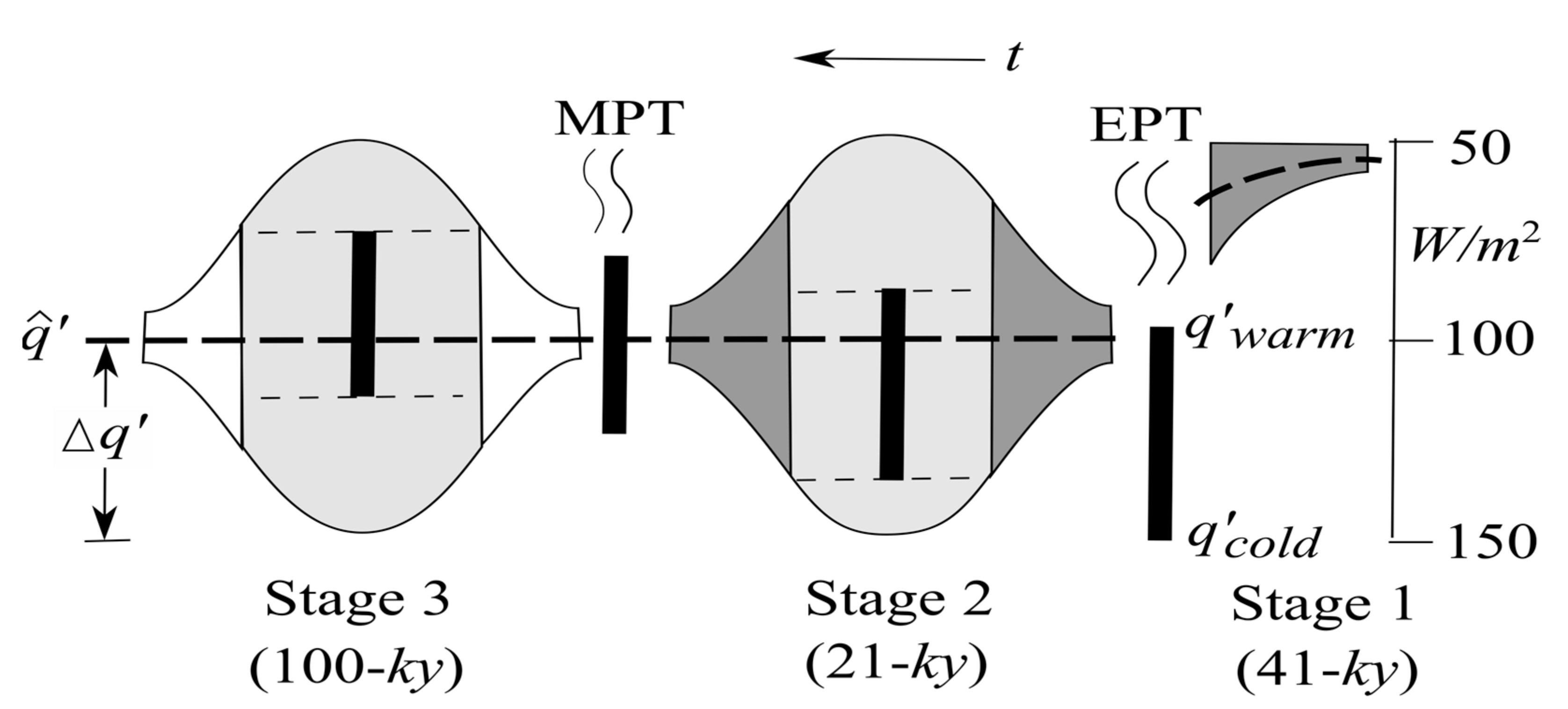
Based on the discussion to follow, I draw in Figure 6 the time evolution of the Pleistocene glacial cycles, which consists of three stages and their transitions. In support of the model deduction, the three stages correspond roughly to those depicted in [89] and their transitions, the early and middle Pleistocene transitions identified by [90]. For each stage, I sketch the forcing envelope (of time-mean and amplitude , neglecting periods of the obliquity and precession) and its enclosed shades signify varied ice signals. The vertical bars are bistable intervals (4)–(5), which move upward (that is, of decreasing magnitude) by the Pleistocene cooling.
At Stage 1 in the early Pleistocene, there is little ice–albedo feedback to effectuate the precession forcing (Section 3.1), so the ice signal is simply that of the polar cap varying linearly with obliquity. The forcing envelope is dark-shaded to signify the 41-ky interglacial cycles, which is identified with the time before 1.5 Ma. The Pleistocene cooling would activate the ice–albedo feedback, hence the precession forcing, with both attaining a maximum when the deepest precession trough exceeds the cold threshold (4) to generate the glacial state. This being the precondition for the full-fledged precession forcing that defines Stage 2, I thus set:
as the marker for its onset. For the forcing shown in the figure, this marker is 75 , and if one assumes a linear cooling of 10 °C from 1.5 Ma to the present and a global convective flux of 100 at 1.5 Ma, this marker would be crossed at 0.9 Ma according to (15). As such, I set 1.5 to 1 Ma as the model-deduced early Pleistocene transition (EPT) from Stage 1 to 2 when the precession forcing gradually emerges by the activation of the ice-albedo feedback. Since such feedback primarily depresses the precession troughs (Section 3.1), the precessional broadening of the forcing, hence the ice-volume envelope during the EPT, would manifest mainly in the deepening of the latter’s centerline, which indeed is a pronounced feature in observations [91].
Stage 2 is defined by the full-fledged precession forcing (hence modulated by eccentricity) when the bistable centerline still lies below the forcing centerline. Although glacial states are now generated by precession troughs during high eccentricity, they are invariably nullified by next precession peaks, and the phase span of this bistable oscillation is light-shaded to signify the presence of glacial ice sheet. Outside this phase span, the precession troughs no longer clear the cold threshold so there is only interglacial ice signal (hence dark-shaded). Stage 2 thus is dominated by 21-ky G/IG cycles, which, however, undergo qualitative change when the continuing cooling would elevate the bistable centerline to cross the forcing centerline, which defines Stage 3.
At Stage 3, there are again bistable oscillations during high eccentricity indicated by the light shade, outside of which however the precession peaks no longer clear the warm transition, so the glacial state would persist through the low eccentricity to propel full growth of the ice sheet to mid-latitudes (hence unshaded, defining our ice age). Stage 3 is thus dominated by 100-ky ice-age cycle, and by equating bistable and forcing centerlines, I drive the following marker for its onset:
Based on Figure 6, it has a value of 61 and is crossed around 0.5 Ma according to (15). Making allowance for the transition, we thus set 1 to 0.7 Ma as the duration of Stage 2 and 0.7 to 0.5 Ma as MPT from Stage 2 to 3.
With above depiction of the three stages, power spectra would shift from that dominated by the obliquity to the emergence of the precession to that dominated by the eccentricity, a deduction that is consistent with their observed change [64,89,90]. Differing from previous conjectures, however, I have provided specific transition markers in terms of time-mean and amplitude of the orbital forcing, and their deduced timings are broadly in accord with the observed ones. For a coarser depiction, one may combine EPT, Stage 2 and MPT into a broader MPT from 41- to 100-ky cycles, which would span 1.5 to 0.5 Ma, also consistent with its traditional designation [23]. Although the model-deduced transition timings depend on Pleistocene cooling, which is far from being linear, they are nonetheless inevitable, hence a robust outcome of the model physics.
To recap, since bistable interval of the orbital forcing is set by the global convective flux that is lowered during Pleistocene cooling on account of the global heat balance, I have derived specific markers for transitions from obliquity- to eccentricity-dominated glacial cycles, which underscore their inevitability and may explain the observed timing.
3.5. Timeseries
To visualize the glacial cycles, I next present generic timeseries calculated for Stage 2 and 3 (there is no need to show Stage 1 characterized by interglacial signals linear in the obliquity forcing). Since the ice–albedo feedback hence the precession forcing is fully operative during these two stages, the model forcing can be approximated by the MI (Section 3.1), which is set to:
where the time-mean is 100, obliquity () has a period of 41 ky and amplitude , and precessions ( and 3) have periods of 18.5 and 23 ky with amplitudes 20 , respectively, which renders a 21 ky precession modulated by 95 ky eccentricity. Together, they result in a forcing amplitude of , as shown in Figure 6. Since MI is only a proxy of the forcing (Section 3.1), above amplitudes need not be precise.
With the above forcing, our climate model would produce (time-varying) ‘equilibrium’ cold-box SST (Section 2.2) and ice margin (Section 3.3), which are now subscripted ‘eq’ for distinction. To calculate the timeseries, we integrate the relaxation equations:
and:
where the time constant for temperature is the MEP adjustment time of 1 ky and is the time constant for the ice margin, which I distinguish between ice advance/retreat. The ice advance is limited by accumulation: a rate of 0.3 for example would build up an ice sheet 3 km high in 10 ky, which is set to be the ice advance time constant; since the melt rate is an order of magnitude greater than the accumulation rate (11), I set the ice retreat time constant to be 1 ky. The relaxation equations being linear, using different time constants merely affects the lag of the timeseries but produces no material difference.
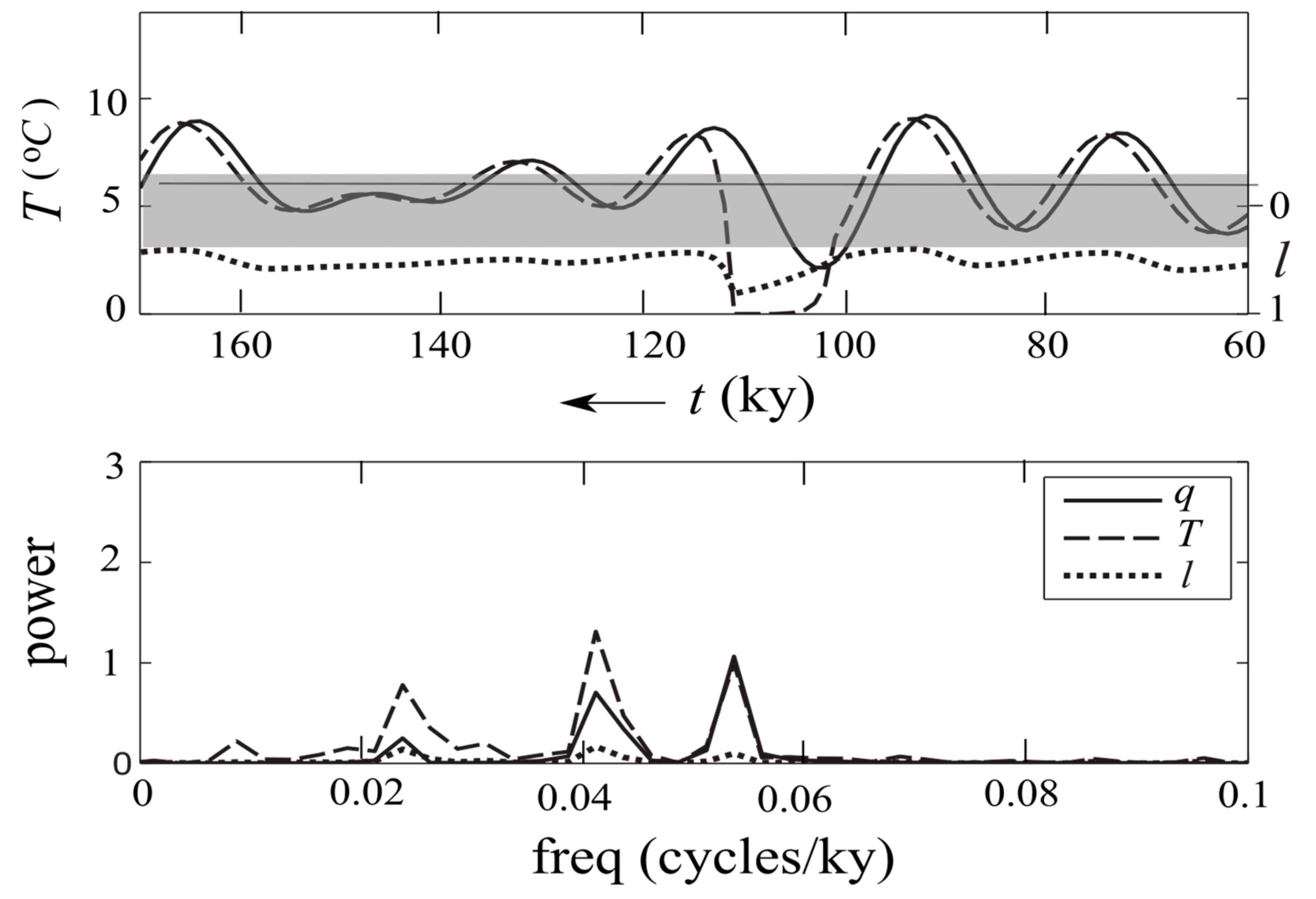
I show in Figure 7 timeseries (time t proceeds to the left) and power spectra of the forcing (q, in equivalent temperature, the solid line), the cold-box SST (T, the dashed line) and ice margin (l, in fractional extension into the subpolar ocean, the dotted line) for Stage 2. For illustration, the global convective flux is set at 69 , same as in Figure 6, a choice that has no import on the generic glacial behavior of the stage. The integration is initiated at warm MEP and carried forward for 400 ky. Since the timeseries equilibrates within the first eccentricity cycle, only the last one needs to be shown. The upper axis represents the global absorbed SW flux and SST ( = 14 °C), and the forcing is expressed in its temperature equivalent (that is, divided by air–sea transfer coefficient, so 100 deficit, for example, would convert to 8 °C below the global SST) with its time-mean indicated by the thin horizontal line, the ice margin is its fractional extension into the subpolar ocean, and the shaded horizonal bar marks the bistable interval (the vertical bar in Figure 6).
It is seen that the forcing resembles the observed summer insolation [69] (their figure 3a) and expectedly contains no power at the eccentricity period. Only one precession trough during high eccentricity has exceeded the cold threshold to induce the glacial state characterized by freezing-point SST. Other than this single glacial episode lasting half the precession period, the interglacial SST simply tracks the forcing with slight delay accompanied by small polar cap variation. Given the short duration of the glacial state, SST and ice margin spectra show no appreciable power at the eccentricity period.
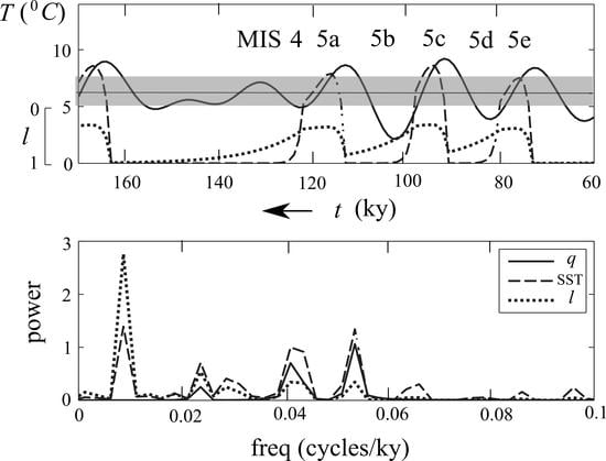
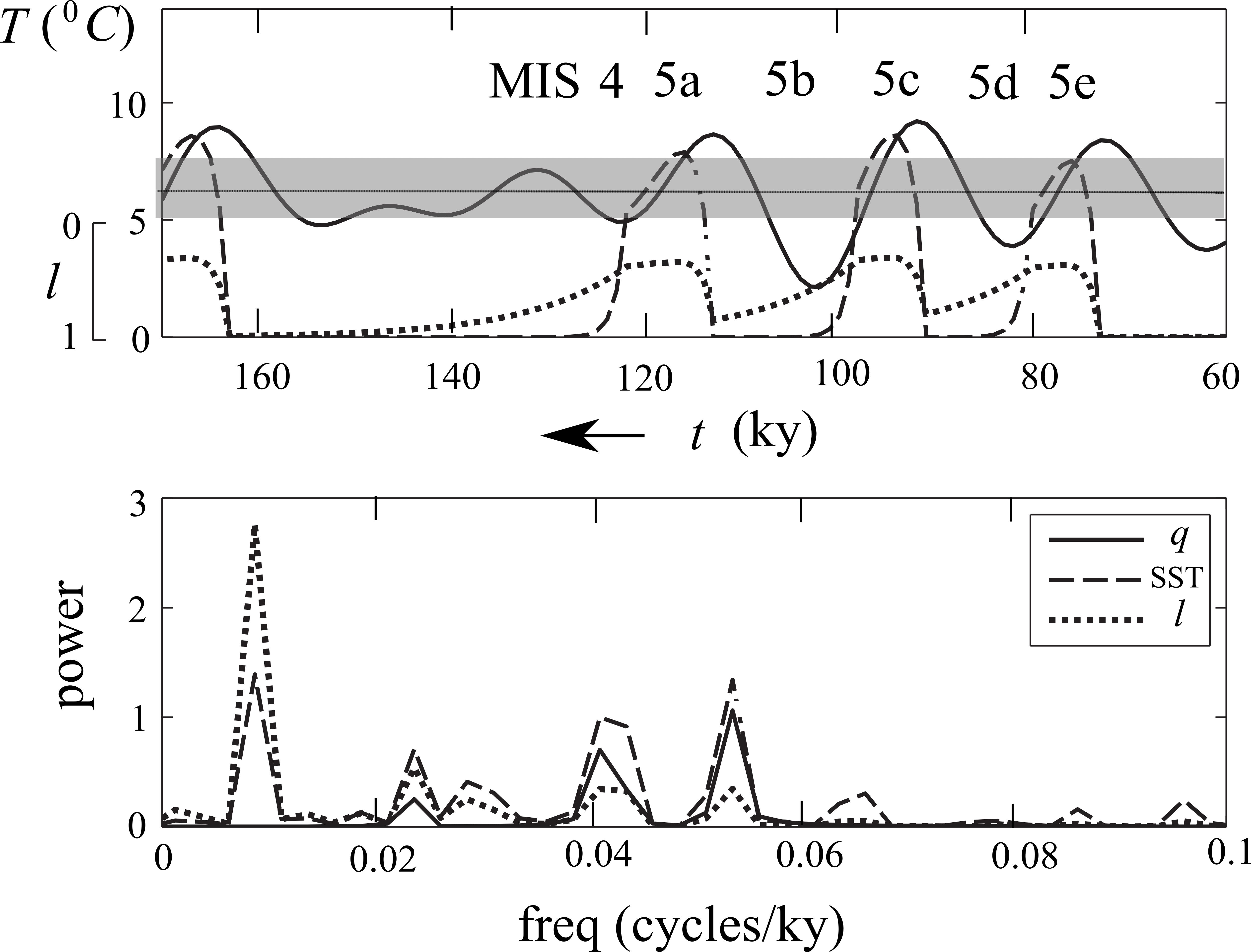
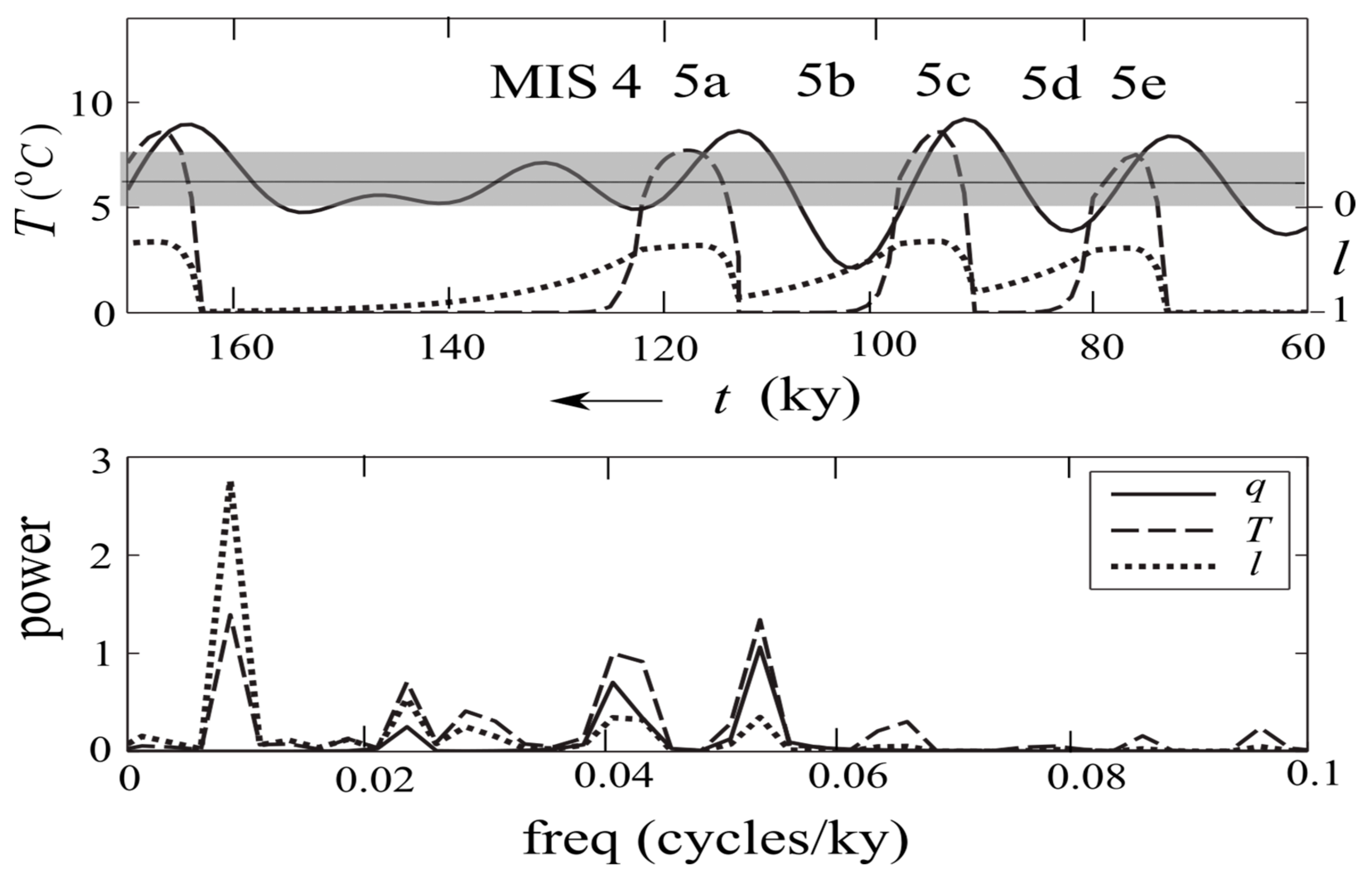
I show in Figure 8 the timeseries and power spectra of Stage 3, for which the global convective flux is set to 56 , same as in Figure 6, a choice again has no import on the generic glacial cycle of the stage. It is seen that the timeseries differ qualitatively from that of Stage 2; there are episodes of interglacial during high precession peaks, which, however, always revert to glacial by the next precession trough, but as eccentricity decreases, the lowered precession peak no longer clears the warm threshold, so the glacial state would persist through the low eccentricity. The prolonged coldness allows the ice sheet to grow to the subtropical front representing the LIS, which defines the ice age. Like Stage 2, the SST and ice-margin spectra retain the precession and obliquity peaks, but as a dramatic difference, they now show a strong eccentricity peak, a contrast seen distinctly in observation [89] (their figure 3).
The timeseries of Stage 3 bears sufficient resemblance to the last ice-age cycle to allow labeling of the observed marine isotope stages (MIS), which thus may be interpreted by the model physics as follows. The cold substages are characterized by freezing-point subpolar water, as seen in the polar front migrating to mid-latitudes and the appearance of polar species in the subpolar water [92,93]. Although the ice sheet growth is limited by the half precession period, it has nevertheless reached half-way to the mid-latitude front, as can be inferred from the observed sea level change and ice-rafted debris (IRD) predicated on a substantial ice sheet [8]. Lending support to the modelled substages being representative of warm/cold branches, the observed SST covaries with the North Atlantic Deep Water (NADW) formation and salinity [7,23,62], as expected from Figure 2. Unlike preceding cold substages, MIS 4 is not reversed due to the decreasing eccentricity, which thus marks the onset of the ice age when ice sheet would grow to the subtropical front [94].
To recap, despite its extreme crudeness, our minimal model has nonetheless reproduced the last ice-age cycle characterized by precessional MIS during high eccentricity and an ice age spanning the low eccentricity. The former is due to large amplitude forcing traversing the bistable interval of the ocean, and the latter is when the lowered precession peak no longer clears the warm threshold in reactivating the MOC. The resemblance with the observed signal supports its interpretation by the model physics.
4. Resolving Pleistocene Glacial Puzzles
Our minimal model may resolve prevailing Pleistocene puzzles, as highlighted below:
- 41-ky problem: since the ocean is forced by the absorbed SW flux, the absence of ice–albedo feedback in the relatively warm early Pleistocene naturally filters out the precession forcing on account of the Kepler’s second law. On the other hand, since the sea-level snowline remains landward of the Arctic Ocean because of the perennial ice, there is always a (continental) polar cap to facilitate the 41-ky obliquity signal [43];
- 100-ky problem: the active ice–albedo feedback in late Pleistocene has nullified Kepler’s second law in instituting the precession forcing modulated by eccentricity. Because of the atmospheric coupling, an eddying ocean is bistable, which translates to bistable ice states of polar cap and LIS. The latter, however, is attained only during low eccentricity when precession peaks no longer clear the warm threshold, thus allowing a prolonged coldness that defines the ice age. This results in 100-ky ice-age cycles paced by eccentricity [95,96];
- MPT problem: the bistable interval is set by the global convective flux, which is lowered during Pleistocene cooling on account of the surface heat balance. Combined with increasing ice–albedo feedback, it segregates the 41- and 100-ky cycles to early and late Pleistocene, respectively, resulting in their mid-Pleistocene transition. Differing from previous conjectures, however, our model has produced specific markers of the MPT (Equations (16) and (17)), which are broadly in accord with the observed timings [23];
- 400-ky problem: so long as the ice-age is already paced by eccentricity of the shorter 100-ky period, the amplitude of the ice-age cycles would be set by the bistable ice states hence unaffected by the longer-period 400-ky eccentricity even though it has comparable amplitude as the shorter one [89];
- Stage-11 problem: despite bistable ice states, a smaller eccentricity would lengthen the ice age to augment the ice signal, thus resolving the Stage-11 problem [89]. By the same token, the time-varying power of the 100-ky eccentricity would anti-correlate with that of the ice-age cycle, as noted by [97], which thus need not involve unknown climate feedback;
- Variable termination problem: Since onset and termination of the ice age are threshold phenomena, both can be off by one precession period depending on the precise timing, the ice-age cycles thus may vary between 80- and 120-ky [98];
- Polar synchronization problem: with Antarctica iced over since late Miocene, it exerts no ice–albedo feedback in instituting the precession forcing—irrespective of its seasonal insolation being anti-phase with its northern counterpart [99]. Then with the glacial cycles dominated by the northern ice sheet, it would feedback into the global balance [88] to synchronize the Antarctic climate, as suggested by its slight lag [96].
Various mechanisms have been proposed in the past in solving these puzzles, our theory is notable in that it resolves them in a single dynamical framework and additionally, differing from previous conjectures, it has produced specific markers of the MPT that may account for the observed timing.
5. Discussion
The central hypotheses of our theory are that the ocean is the intermediary of the orbital forcing of the ice sheet, and that the ocean is inherently turbulent to be propelled toward MEP. To isolate the essential physics and lessen the allowance for tunning, I have presented a minimal model to allow its more stringent test against observations. With this perspective, simplifying assumptions are justified so long as they do not alter the basic closure to materially impact the model derivation.
With the ocean playing a key role of the glacial cycles, one obvious question concerns the diapycnal diffusivity typically regarded as an enabler of the MOC in overcoming the potential-energy barrier [55]. This conception however does not conflict with our MOC being propelled by MEP adjustment regardless the diapycnal diffusivity (Section 2.2); this is because the potential energy barrier depends also on the thermocline depth, which is no longer constrained by the laminar momentum balance—a degree of freedom that is in effect closed by the MEP adjustment. In other words, varying diapycnal diffusivity would only regulate the thermocline depth without impacting the MOC hence the model derivation.
Since MEP is a global property, it negates the relevance of eddy diffusivity diagnosed from observation or derived from local turbulence closure, so to capture MEP adjustment from primitive equation models, there seems to be no substitute than resolving eddies, which obviously poses a daunting challenge to glacial-cycle simulations because of the long integration needed. A phenomenological approach, however, may be feasible by implementing the MEP adjustment equation of [21] explicitly (his equation (23)) but replacing the admittance by the equivalent diapycnal diffusivity because of their power law dependence. The equation now states:
where is the fluctuation amplitude set by density stratification (a ratio of the decorrelation distance of eddy shedding to basin width), n, the exponent of the power law (about 0.5, [18]) and , the entropy production. Given a diapycnal diffusivity, one may calculate the entropy production (a simpler task via the boundary entropy flux, see Section 2.2) and from its neighboring realizations of slightly different diapycnal diffusivity, one may calculate the right-hand side of the equation to allow a forward marching of the climate, which should propel toward MEP. Differing from prior studies [100,101,102], however, our selection of the diapycnal diffusivity as the optimizing parameter is justifiable by the fluctuation theorem.
In conclusion, I have demonstrated through a minimal model that the mere positing of an eddying ocean as the intermediary of the orbital forcing of the ice sheet is sufficient to account for Pleistocene glacial cycles and resolve many longstanding puzzles.
Funding
This research received no external funding.
Data Availability Statement
No datasets were generated or analyzed.
Acknowledgments
This paper has benefited from comments of anonymous reviewers.
Conflicts of Interest
This author declares no conflict of interest.
Abbreviations
| DNS | Direct numerical simulation |
| EL | Equilibrium line |
| ELA | Equilibrium-line altitude |
| EPT | Early Pleistocene transition |
| FT | Fluctuation theorem |
| G/IG | Glacial/interglacial |
| IRD | Ice-rafted debris |
| LGM | Last glacial maximum |
| LIS | Laurentide ice sheet |
| LW | Long-wave |
| Ma | Million years ago |
| MEP | Maximum entropy production |
| MI | Milankovitch insolation |
| MIS | Marine isotope stage |
| MOC | Meridional overturning circulation |
| MPT | Mid-Pleistocene transition |
| NADW | North Atlantic Deep Water |
| NT | Nonequilibrium thermodynamics |
| PDD | Positive degree-day |
| SAT | Surface-air temperature |
| SST | Sea-surface temperature |
| SW | Short-wave |
Appendix A
| Global ice cover | |
| Ablation | |
| Accumulation | |
| Forcing amplitudes | |
| Bo | Ratio of sensible to latent heat transports |
| c | Ice dynamics parameter ( |
| Specific heat of water | |
| Saturation vapor pressure | |
| Atmospheric energy transport | |
| Gravitational acceleration () | |
| h | Ice height |
| ELA | |
| K | MOC strength |
| [K] | Scale of K () |
| x-coordinate of EL | |
| , | x-coordinate of ice margin |
| Equilibrium l | |
| Latent heat of sublimation () | |
| Melt rate () | |
| Exponent of admittance power law | |
| Global absorbed SW flux | |
| Cold-box deficit of absorbed SW flux | |
| Dimensional | |
| Cold-box deficit of convective flux | |
| Time-mean of () | |
| Amplitude of () | |
| Scale of ( | |
| Global convective flux | |
| Global surface LW flux | |
| Cold-transition threshold | |
| Warm-transition threshold | |
| Cold-box salinity deficit | |
| Scale of = 1.79) | |
| Entropy production rate | |
| Sv | Sverdrup () |
| Global SST (=14 °C) | |
| Cold-box SST deficit | |
| Dimensional | |
| Scale of | |
| Equilibrium | |
| Freezing-point | |
| w | Half continental width |
| Thermal expansion coefficient ( | |
| Air-sea transfer coefficient (, [21]) | |
| Saline contraction coefficient ( | |
| Lapse rate | |
| Fluctuation amplitude | |
| Cold-box density surplus | |
| Scale of ( | |
| Ice density () | |
| Water density () | |
| Yield stress () | |
| Ice time constant for retreat/advance) | |
| Temperature time constant | |
| Melt rate per degree temperature (=0.8 my−1 °C−1) | |
| Moisture parameter | |
| Dimensionless moisture parameter (0.3, [21]) | |
| Diapycnal diffusivity |
References
- Hays, J.D.; Imbrie, J.; Shackleton, N.J. Variations in the Earth’s orbit: Pacemaker of the ice ages. Science 1976, 194, 1121–1132. [Google Scholar] [CrossRef]
- Berger, A. Spectrum of climatic variations and their causal mechanisms. Geophys. Surv. 1979, 3, 351–402. [Google Scholar] [CrossRef]
- Milankovitch, M. Canon of Insolation and the Ice-Age Problem; R Serb Acad Spec 1941, Publ 132 (Translated from German); Israel Program for Scientific Translations: Jerusalem, Israel, 1969. [Google Scholar]
- Donohoe, A.; Battisti, D.S. The seasonal cycle of atmospheric heating and temperature. J. Clim. 2013, 26, 4962–4980. [Google Scholar] [CrossRef]
- Peixoto, J.P.; Oort, A.H. Physics of Climate; American Institute of Physics: New York, NY, USA, 1992. [Google Scholar] [CrossRef]
- Dansgaard, W.; Johnsen, S.; Clausen, H.B.; Dahl-Jensen, D.; Gundestrup, N.; Hammer, C.U.; Hvldberg, C.S.; Steffensen, J.P.; Sveinbjornsdottir, A.E.; Jouzel, J.; et al. Evidence for general instability of past climate from a 250-kyr ice-core record. Nature 1993, 364, 218–220. [Google Scholar] [CrossRef]
- Labeyrie, L.; Vidal, L.; Cortijo, E.; Paterne, M.; Arnold, M.; Duplessy, J.C.; Vautravers, M.; Labracherie, M.; Dupart, J.; Turon, J.L.; et al. Surface and deep hydrology of the Northern Atlantic Ocean during the last 150,000 years. Philos. Trans. R. Soc. Lond. Ser. B 1995, 348, 255–264. [Google Scholar] [CrossRef]
- Chapman, M.R.; Shackleton, N.J. Global ice-volume fluctuations, North Atlantic ice-rafting events, and deep-ocean circulation changes between 130 and 70 ka. Geology 1999, 27, 795–798. [Google Scholar] [CrossRef]
- Petit, J.R.; Jouzel, J.; Raynaud, D.; Barkov, N.I.; Barnola, J.M.; Basile, I.; Bender, M.; Chappellaz, J.; Davis, M.; Delaygue, G.; et al. Climate and atmospheric history of the past 420,000 years from the Vostok ice core, Antarctica. Nature 1999, 399, 429–436. [Google Scholar] [CrossRef]
- Shackleton, N. The 100,000-year ice-age cycle identified and found to lag temperature, carbon dioxide, and orbital eccentricity. Science 2000, 289, 1897–1902. [Google Scholar] [CrossRef]
- Broecker, W.S.; Denton, G.H. The role of ocean-atmosphere reorganization in glacial cycles. Geochim. Cosmochim. Acta 1989, 53, 2465–2501. [Google Scholar] [CrossRef]
- Birchfield, G.E.; Weertman, J.; Lunde, A.T. A paleoclimate model of Northern Hemisphere ice sheets. Quat. Res. 1981, 15, 126–142. [Google Scholar] [CrossRef]
- Gallée, H.; Van Yperselb, J.P.; Fichefet, T.; Marsiat, I.; Tricot, C.; Berger, A. Simulation of the last glacial cycle by a coupled, sectorially averaged climate-ice sheet model: 2. Response to insolation and CO2 variations. J. Geophys. Res. 1992, 97, 15713–15740. [Google Scholar] [CrossRef]
- Berger, A.; Li, X.; Loutre, M. Modeling northern hemisphere ice volume over the last 3 ma. Quat. Sci. Rev. 1999, 18, 1–11. [Google Scholar] [CrossRef]
- Abe-Ouchi, A.; Segawa, T.; Saito, F. Climatic conditions for modelling the Northern Hemisphere ice sheets throughout the ice age cycle. Clim. Past 2007, 3, 423–438. [Google Scholar] [CrossRef]
- Auer, S.J. Five-year climatological survey of the Gulf Stream system and its associated rings. J. Geophys. Res. 1987, 92, 11709–11726. [Google Scholar] [CrossRef]
- Lozier, M.S. Deconstructing the conveyer belt. Science 2010, 328, 1507–1511. [Google Scholar] [CrossRef]
- Dalan, F.; Stone, P.; Kamenkovich, I.V.; Scott, J.R. Sensitivity of the Ocean’s Climate to Diapycnal Diffusivity in an EMIC. Part I: Equilibrium State. J. Clim. 2005, 18, 2460–2481. [Google Scholar] [CrossRef]
- Rahmstorf, S.; Crucifix, M.; Ganopolski, A.; Goosse, M.; Kamenkovich, I.; Knutti, R.; Lohmann, G.; Marsh, R.; Mysak, L.A.; Wang, Z.; et al. Thermohaline circulation hysteresis: A model intercomparison. Geophys. Res. Lett. 2005, 32, L23605. [Google Scholar] [CrossRef]
- Ganopolski, A.; Brovkin, V. Simulation of climate, ice sheets and CO2 evolution during the last four glacial cycles with an Earth system model of intermediate complexity. Clim. Past 2017, 13, 1695–1716. [Google Scholar] [CrossRef]
- Ou, H.W. Thermohaline circulation: A missing equation and its climate change implications. Clim. Dyn. 2018, 50, 641–653. [Google Scholar] [CrossRef]
- Elkibbi, M.; Rial, J.A. An outsider’s review of the astronomical theory of the climate: Is the eccentricity-driven insolation the main driver of the ice ages? Earth Sci. Rev. 2001, 56, 161–177. [Google Scholar] [CrossRef]
- Clark, P.U.; Archer, D.; Pollard, D.; Blum, J.D.; Rial, J.A.; Brovkin, V.; Mix, A.C.; Pisias, N.G.; Roy, M. The middle Pleistocene transition: Characteristics, mechanisms, and implications for long-term changes in atmospheric pCO2. Quat. Sci. Rev. 2006, 25, 3150–3184. [Google Scholar] [CrossRef]
- Imbrie, J.; Imbrie, J.Z. Modeling the Climatic Response to Orbital Variations. Science 1980, 207, 943–953. [Google Scholar] [CrossRef] [PubMed]
- Oerlemans, J. Glacial cycles and ice-sheet modelling. Clim. Change 1982, 4, 353–374. [Google Scholar] [CrossRef]
- Pollard, D. A coupled climate-ice sheet model applied to the Quaternary ice ages. J. Geophys. Res. 1983, 88, 7705–7718. [Google Scholar] [CrossRef]
- Pelletier, J.D. Coherence resonance and ice ages. J. Geophys. Res. 2003, 108, 4645. [Google Scholar] [CrossRef]
- Ghil, M. Cryothermodynamics: The chaotic dynamics of paleoclimate. Phys. D Nonlinear Phenom. 1994, 77, 130–159. [Google Scholar] [CrossRef]
- Wunsch, C. The spectral description of climate change including the 100 ky energy. Clim. Dyn. 2003, 20, 353–363. [Google Scholar] [CrossRef]
- Tziperman, E.; Raymo, M.E.; Huybers, P.J.; Wunsch, C. Consequences of pacing the Pleistocene 100 kyr ice ages by nonlinear phase locking to Milankovitch forcing. Paleoceanography 2006, 21, 1–11. [Google Scholar] [CrossRef]
- Ravelo, A.N.; Andreasen, D.H.; Lyle, M.; Lyle, A.O.; Wara, M.W. Regional climate shifts caused by gradual global cooling in the Pliocene epoch. Nature 2004, 429, 263–267. [Google Scholar] [CrossRef]
- Saltzman, B.; Hansen, A.; Maasch, K. The late Quaternary glaciations as the response of a three-component feedback system to Earth-orbital forcing. J. Atmos. Sci. 1984, 41, 3380–3389. [Google Scholar] [CrossRef]
- Paillard, D. The timing of Pleistocene glaciations from a simple multiple-state climate model. Nature 1998, 391, 378–381. [Google Scholar] [CrossRef]
- Imbrie, J.Z.; Imbrie-Moore, A.; Lisiecki, L.E. A phase-space model for Pleistocene ice volume. Earth Planet. Sci. Lett. 2011, 307, 94–102. [Google Scholar] [CrossRef]
- Crucifix, M. Why could ice ages be unpredictable? Clim. Past 2013, 9, 2253–2267. [Google Scholar] [CrossRef]
- Daruka, I.; Ditlevsen, P.D. A conceptual model for glacial cycles and the middle Pleistocene transition. Clim. Dyn. 2016, 46, 29–40. [Google Scholar] [CrossRef]
- Verbitsky, M.Y.; Crucifix, M.; Volobuev, D.M. A theory of Pleistocene glacial rhythmicity. Earth Syst. Dyn. 2018, 9, 1025–1043. [Google Scholar] [CrossRef]
- Willeit, M.; Ganopolski, A.; Calov, R.; Brovkin, V. Mid-Pleistocene transition in glacial cycles explained by declining CO2 and regolith removal. Sci. Adv. 2019, 5, eaav7337. [Google Scholar] [CrossRef]
- Honisch, B.; Hemming, N.G.; Archer, D.; Siddall, M.; McManus, J.F. Atmospheric carbon dioxide concentration across the mid-Pleistocene transition. Science 2009, 324, 1551–1554. [Google Scholar] [CrossRef] [PubMed]
- Weertman, J. Milankovitch solar radiation variations and ice age ice sheet sizes. Nature 1976, 261, 17–20. [Google Scholar] [CrossRef]
- Calov, R.; Ganopolski, A. Multistability and hysteresis in the climate-cryosphere system under orbital forcing. Geophys. Res. Lett. 2005, 32, L21717. [Google Scholar] [CrossRef]
- Berger, A.; Loutre, M.F. Modeling the 100-kyr glacial–interglacial cycles. Glob. Planet. Change 2010, 72, 275–281. [Google Scholar] [CrossRef]
- Raymo, M.E.; Nisancioglu, K.H. The 41 kyr world: Milankovitch’s other unsolved mystery. Paleoceanography 2003, 18. [Google Scholar] [CrossRef]
- Kucera, M.; Weinelt, M.; Kiefer, T.; Pflaumann, U.; Hayes, A.; Weinelt, M.; Chen, M.T.; Mix, A.C.; Barrows, T.T.; Cortijo, E.; et al. Reconstruction of sea-surface temperatures from assemblages of planktonic foraminifera: Multi-technique approach based on geographically constrained calibration data sets and its application to glacial Atlantic and Pacific Oceans. Quat. Sci. Rev. 2005, 24, 951–998. [Google Scholar] [CrossRef]
- Stommel, H. Thermohaline convection with two stable regimes of flow. Tellus 1961, 13, 224–230. [Google Scholar] [CrossRef]
- Marotzke, J.; Stone, P. Atmospheric transports, the thermohaline circulation, and flux adjustments in a simple coupled model. J. Phys. Oceanogr. 1995, 25, 1350–1364. [Google Scholar] [CrossRef]
- Manabe, S.; Stouffer, R.J. Two stable equilibria of a coupled ocean-atmosphere model. J. Clim. 1988, 1, 841–866. [Google Scholar] [CrossRef]
- Crooks, G.E. Entropy production fluctuation theorem and the nonequilibrium work relation for free energy differences. Phys. Rev. 1999, 60, 2721–2726. [Google Scholar] [CrossRef]
- Ou, H.W. Possible bounds on the earth’s surface temperature: From the perspective of a conceptual global-mean model. J. Clim. 2001, 14, 2976–2988. [Google Scholar] [CrossRef]
- Ozawa, H.; Ohmura, A.; Lorenz, R.D.; Pujol, T. The second law of thermodynamics and the global climate system: A review of the maximum entropy production principle. Rev. Geophys. 2003, 41, 1018. [Google Scholar] [CrossRef]
- Kleidon, A. Non-equilibrium thermodynamics and maximum entropy production in the Earth system: Applications and implications. Naturwissenschaften 2009, 96, 653–677. [Google Scholar] [CrossRef]
- Evans, D.J.; Searle, D.J. The fluctuation theorem. Adv. Phys. 2002, 51, 1529. [Google Scholar] [CrossRef]
- Wang, G.M.; Sevick, E.M.; Mittag, E.; Searles, D.J.; Evans, D.J. Experimental demonstration of violations of the Second Law of Thermodynamics for small systems and short time scales. Phys. Rev. Lett. 2002, 89, 050601. [Google Scholar] [CrossRef] [PubMed]
- Hogg, A.M.; Gayen, B. Ocean gyres driven by surface buoyancy forcing. Geophys. Res. Lett. 2020, 47, e2020GL088539. [Google Scholar] [CrossRef]
- Colin de Verdière, A. Buoyancy driven planetary flows. J. Mar. Res. 1988, 46, 2215–2265. [Google Scholar] [CrossRef]
- Ou, H.W. Meridional thermal field of a coupled ocean-atmosphere system: A conceptual model. Tellus A Dyn. Meteorol. Oceanogr. 2006, 58, 404–415. [Google Scholar] [CrossRef]
- Ou, H.W. A theory of abrupt climate changes: Their genesis and anatomy. Geosciences 2022, 12, 391. [Google Scholar] [CrossRef]
- Macdonald, A.M. The global ocean circulation: A hydrographic estimate and regional analysis. Prog. Oceanogr. 1998, 41, 281–382. [Google Scholar] [CrossRef]
- De Vernal, A.; Eynaud, F.; Henry, M.; Hillaire-Marcel, C.; Londeix, L.; Mangin, S.; Matthiessen, J.; Marret, F.; Radi, T.; Rochon, A.; et al. Reconstruction of sea surface conditions at middle to high latitudes of the Northern Hemisphere during the Last Glacial Maximum (LGM) based on dinoflagellate cyst assemblages. Quat. Sci. Rev. 2005, 24, 897–924. [Google Scholar] [CrossRef]
- Gildor, H.; Tziperman, E. Sea ice as the glacial cycles climate switch: Role of seasonal and orbital forcing. Paleoceanography 2000, 15, 605–615. [Google Scholar] [CrossRef]
- Duplessy, J.C.; Shackleton, N.J. Response of global deep-water circulation to Earth’s climatic change 135,000–107,000 years ago. Nature 1985, 316, 500–507. [Google Scholar] [CrossRef]
- Keigwin, L.D.; Curry, W.B.; Lehman, S.J.; Johnsen, S. The role of the deep ocean in North Atlantic climate change between 70 and 130 kyr ago. Nature 1994, 371, 323–326. [Google Scholar] [CrossRef]
- Berger, A.; Loutre, M.F.; Kaspar, F.; Lorenz, S.J. Chapter 2—Insolation during interglacial. In Developments in Quaternary Sciences; Elsevier: Amsterdam, The Netherlands, 2007; Volume 7, pp. 13–27. [Google Scholar] [CrossRef]
- Berger, A. Milankovitch theory and climate. Rev. Geophys. 1988, 26, 624–657. [Google Scholar] [CrossRef]
- Short, D.A.; Mengel, J.G.; Crowley, T.J.; Hyde, W.T.; North, G.R. Filtering of Milankovitch cycles by Earth’s geography. Quat. Res. 1991, 35, 157–173. [Google Scholar] [CrossRef]
- Huybers, P. Early Pleistocene glacial cycles and the integrated summer insolation forcing. Science 2006, 313, 508–511. [Google Scholar] [CrossRef] [PubMed]
- Pollard, D. A simple parameterization for ice sheet ablation rate. Tellus 1980, 32, 384–388. [Google Scholar] [CrossRef]
- Peltier, W.R. Ice age paleotopography. Science 1994, 265, 195–201. [Google Scholar] [CrossRef] [PubMed]
- Berger, A.; Gallee, H.; Li, X.S.; Dutrieux, A.; Loutre, M.F. Ice sheet growth and high-latitudes sea surface temperature. Clim. Dyn. 1996, 12, 441–448. [Google Scholar] [CrossRef]
- Abe-Ouchi, A.; Saito, F.; Kawamura, K.; Raymo, M.E.; Okuno, J.I.; Takahashi, K.; Blatter, H. Insolation-driven 100,000-year glacial cycles and hysteresis of ice-sheet volume. Nature 2013, 500, 190–193. [Google Scholar] [CrossRef]
- Van der Veen, C.I. Fundamentals of Glacier Dynamics, 2nd ed.; CRC Press: Boca Raton, FL, USA, 2013; p. 403. [Google Scholar] [CrossRef]
- Reeh, N. A plasticity theory approach to the steady-state shape of a three-dimensional ice sheet. J. Glaciol. 1982, 28, 431–455. [Google Scholar] [CrossRef]
- Robin, G.D. Ice cores and climatic change. Philos. Trans. R. Soc. Lond. Ser. B 1977, 280, 143–168. [Google Scholar] [CrossRef]
- Ou, H.W. Hydrological cycle and ocean stratification in a coupled climate system: A theoretical study. Tellus 2007, 59, 683–694. [Google Scholar] [CrossRef]
- Ohmura, A.; Reeh, N. New precipitation and accumulation maps for Greenland. J. Glaciol. 1991, 37, 140–148. [Google Scholar] [CrossRef]
- Bromwich, D.H.; Robasky, F.M.; Keen, R.A.; Bolzan, J.F. Modeled variations of precipitation over the Greenland ice sheet. J. Clim. 1993, 6, 1253–1268. [Google Scholar] [CrossRef]
- Alley, R.B.; Meese, D.A.; Shuman, C.A.; Glow, A.J.; Taylor, K.C.; Grouts, P.M.; White, J.W.C.; Ram, M.; Waddington, E.D.; Mayewski, P.A.; et al. Abrupt increase in snow accumulation at the end of the Younger Dryas event. Nature 1993, 362, 527–529. [Google Scholar] [CrossRef]
- Reeh, N. Parameterization of melt rate and surface temperature in the Greenland ice sheet. Polarforschung 1991, 59, 113–128. [Google Scholar]
- Oerlemans, J. The mass balance of the Greenland ice sheet: Sensitivity to climate change as revealed by energy-balance modelling. Holocene 1991, 1, 40–48. [Google Scholar] [CrossRef]
- North, G.R.; Mengel, J.G.; Short, D.A. Simple energy balance model resolving the seasons and the continents: Application to the astronomical theory of the ice ages. J. Geophys. Res. 1983, 88, 6576–6586. [Google Scholar] [CrossRef]
- Carlson, A. Why there was not a Younger Dryas-like event during the Penultimate Deglaciation? Quat. Sci. Rev. 2008, 27, 882–887. [Google Scholar] [CrossRef]
- Oerlemans, J. Model experiments on the 100,000-yr glacial cycle. Nature 1980, 287, 430–432. [Google Scholar] [CrossRef]
- Clark, D.L. Origin, nature and world climate effect of Arctic Ocean ice-cover. Nature 1982, 300, 321–325. [Google Scholar] [CrossRef]
- Ruddiman, W.; Raymo, M. Northern Hemisphere climate regimes during the past 3 Ma: Possible tectonic connections. Philos. Trans. R. Soc. Lond. Ser. B 1988, 318, 411–430. [Google Scholar] [CrossRef]
- Raymo, M.E.; Ruddiman, W.F. Tectonic forcing of late Cenozoic climate. Nature 1992, 1359, 117–122. [Google Scholar] [CrossRef]
- Previdi, M. Radiative feedbacks on global precipitation. Environ. Res. Lett. 2010, 5, 025211. [Google Scholar] [CrossRef]
- Martínez-Botí, M.A.; Foster, G.L.; Chalk, T.B.; Rohling, E.J.; Sexton, P.F.; Lunt, D.J.; Pancost, R.D.; Badger, M.P.; Schmidt, D.N. Plio-Pleistocene climate sensitivity evaluated using high-resolution CO2 records. Nature 2015, 518, 49–54. [Google Scholar] [CrossRef] [PubMed]
- Broccoli, A.J.; Manabe, S. The influence of continental ice, atmospheric CO2, and land albedo on the climate of the last glacial maximum. Clim. Dyn. 1987, 1, 87–99. [Google Scholar] [CrossRef]
- Imbrie, J.; Berger, A.; Boyle, E.; Clemens, S.C.; Duffy, A.; Howard, W.R.; Kukla, G.; Kutzbach, J.; Martinson, D.G.; McIntyre, A.; et al. On the structure and origin of major glaciation cycles 2. The 100,000-year cycle. Paleoceanography 1993, 8, 699–735. [Google Scholar] [CrossRef]
- Lisiecki, L.E.; Raymo, M.E. Plio–Pleistocene climate evolution: Trends and transitions in glacial cycle dynamics. Quat. Sci. Rev. 2007, 26, 56–69. [Google Scholar] [CrossRef]
- Lisiecki, L.E.; Raymo, M.E. A Pliocene-Pleistocene stack of 57 globally distributed benthic δ18O records. Paleoceanography 2005, 20, PA1003. [Google Scholar] [CrossRef]
- Ruddiman, W.F.; McIntyre, A. The North Atlantic Ocean during the last deglaciation. Palaeogeogr. Palaeoclimatol. Palaeoecol. 1981, 35, 145–214. [Google Scholar] [CrossRef]
- McManus, J.F.; Bond, G.C.; Broecker, W.S.; Johnsen, S.; Labeyrie, L.; Higgins, S. High-resolution climate records from the N. Atlantic during the last interglacial. Nature 1994, 371, 326–329. [Google Scholar] [CrossRef]
- Ruddiman, W.F.; McIntyre, A.; Niebler-Hunt, V.; Durazzi, J.T. Oceanic evidence for the mechanism of rapid northern hemisphere glaciation. Quat. Res. 1980, 13, 33–64. [Google Scholar] [CrossRef]
- Raymo, M.E. The timing of major climate terminations. Paleoceanography 1997, 12, 577–585. [Google Scholar] [CrossRef]
- Kawamura, K.; Parrenin, F.; Lisiecki, L.; Uemura, R.; Vimeux, F.; Severinghaus, J.P.; Hutterli, M.A.; Nakazawa, T.; Aoki, S.; Jouzel, J.; et al. Northern Hemisphere forcing of climatic cycles in Antarctica over the past 360,000 years. Nature 2007, 448, 912–916. [Google Scholar] [CrossRef]
- Lisiecki, L.E. Links between eccentricity forcing and the 100,000-year glacial cycle. Nat. Geosci. 2010, 3, 349–352. [Google Scholar] [CrossRef]
- Raymo, M.E.; Oppo, D.W.; Curry, W. The mid-Pleistocene climate transition: A deep sea carbon isotopic perspective. Paleoceanography 1997, 12, 546–559. [Google Scholar] [CrossRef]
- Clark, P.U.; Alley, R.B.; Pollard, D. Northern Hemisphere ice sheet influences on global climate change. Science 1999, 286, 1104–1111. [Google Scholar] [CrossRef]
- Kleidon, A.; Fraedrich, K.; Kunz, T.; Lunkeit, F. The atmospheric circulation and states of maximum entropy production. Geophys. Res. Lett. 2003, 30. [Google Scholar] [CrossRef]
- Kunz, T.; Fraedrich, K.; Kirk, E. Optimisation of simplified GCMs using circulation indices and maximum entropy production. Clim. Dyn. 2008, 30, 803–813. [Google Scholar] [CrossRef]
- Jupp, T.E.; Cox, P.M. MEP and planetary climates: Insights from a two-box climate model containing atmospheric dynamics. Philos. Trans. R. Soc. Lond. Ser. B 2010, 365, 1355–1365. [Google Scholar] [CrossRef] [PubMed]
Figure 1.
The model configuration of a coupled ocean/atmosphere composed of warm/cold masses aligned at mid-latitudes and an ice sheet on continents terminating at an ice-covered Arctic Ocean. The model variables are the cold-box deviations from global means of the absorbed SW flux (), SST (), convective flux (), salinity () and density (), the last drives the MOC (K) involving random eddy exchange across the subtropical front. Total accumulation () and ablation (), both are prognostic, would constrain the ELA () hence its x-coordinate () and ice margin ().

Figure 2.
The regime diagram in which the subpolar water properties (temperature/salinity deficits and density surplus ) are plotted against the MOC (K) (all nondimensionalized). Vertical dashed is the convective bound that divides warm/cold branches and the intersect of the density (thick solid) and MOC (thick dashed) lines specifies the climate states (solid ovals, the open oval being an unrealized saddle point). The MOC line is subjected to microscopic fluctuations (shaded cone) to pivot on millennial timescale toward MEP (rectangles). Temperature markings on the ordinate are the forcing (), the global convective flux () and the freezing point ().

Figure 3.
The evolution of the warm MEP (solid arrows from solid to open rectangles) when the forcing deficit (hence temperature and density lines) is raised and the cold MEP (dashed arrows from solid to open ovals) when is lowered. Vertical dashed lines are convective bounds, thick dashed lines are the MOC lines of the cold MEP, and shaded cone signifies microscopic fluctuations.

Figure 4.
Aligned SST, summer SAT and snowline (thick solid) in the subpolar zone for the interglacial. The intersect of the snowline with the ELA (thick dashed) specifies the margin of the polar cap (medium-shaded), which varies with the forcing as it pivots the snowline (dark-shaded cone). For the glacial, the snowline is flush with the sea level, so the LIS (light-shaded) extends to the subtropical front. The misconceived lifting of the snowline (dash-dotted) would yield ice-free continent, which however is untenable for ice-covered Arctic Ocean.

Figure 5.
The positive degree-day (PDD) plotted against July temperature for seasonal amplitude of 10 °C (solid line, taken from [78] (his figure 2). The corresponding melt rate is marked on the right ordinate and approximated by the straight dashed line (license link: https://creativecommons.org/licenses/by/4.0/, accessed on 1 January 2023).

Figure 6.
A schematic of the Pleistocene evolution of the forcing envelope and ice-volume signal (varying shades) deduced from our model, which consists of three stages and their transitions. The vertical bars are bistable intervals, which move upward by Pleistocene cooling. The three stages are dominated successively by 41-ky interglacial cycles (dark-shaded), 21-ky G/IG cycles (light-shaded) and 100-ky ice-age cycles (unshaded).

Figure 7.
Timeseries (time t proceeds to the left) and power spectra of the forcing (q, in equivalent temperature), subpolar SST (T) and ice margin (l, in fractional extension into the subpolar ocean) for Stage 2 of Figure 6. The upper axis marks the global absorbed SW flux and SST, the forcing is expressed in its temperature equivalent with the time-mean forcing (horizonal line) and bistable interval (shaded bar) indicated. There is only one episode of the glacial state lasting half precession period, so SST and ice margin spectra exhibit only precession and obliquity peaks, just like the forcing.

Figure 8.
Same as Figure 7 but for Stage 3 of Figure 6. There are G/IG cycles during high eccentricity corresponding to the observed marine isotope stages, and a glacial state spanning the low eccentricity to propel full growth of the ice sheet to the subtropical front. In contrast to Stage 2, the SST and ice-margin spectra exhibit strong eccentricity peaks absent in the forcing.

Disclaimer/Publisher’s Note: The statements, opinions and data contained in all publications are solely those of the individual author(s) and contributor(s) and not of MDPI and/or the editor(s). MDPI and/or the editor(s) disclaim responsibility for any injury to people or property resulting from any ideas, methods, instructions or products referred to in the content. |
© 2023 by the author. Licensee MDPI, Basel, Switzerland. This article is an open access article distributed under the terms and conditions of the Creative Commons Attribution (CC BY) license (https://creativecommons.org/licenses/by/4.0/).
Share and Cite
MDPI and ACS Style
Ou, H.-W. A Theory of Orbital-Forced Glacial Cycles: Resolving Pleistocene Puzzles. J. Mar. Sci. Eng. 2023, 11, 564. https://doi.org/10.3390/jmse11030564
AMA Style
Ou H-W. A Theory of Orbital-Forced Glacial Cycles: Resolving Pleistocene Puzzles. Journal of Marine Science and Engineering. 2023; 11(3):564. https://doi.org/10.3390/jmse11030564
Chicago/Turabian StyleOu, Hsien-Wang. 2023. "A Theory of Orbital-Forced Glacial Cycles: Resolving Pleistocene Puzzles" Journal of Marine Science and Engineering 11, no. 3: 564. https://doi.org/10.3390/jmse11030564
Note that from the first issue of 2016, this journal uses article numbers instead of page numbers. See further details here.