Study Regarding the Influence of Blade Rotation Angle Deviations on the Hydraulic Pulsation Characteristics of a Mixed-Flow Pump

Abstract

Mixed-flow pumps with adjustable blades are widely used in municipal, agricultural, and hydropower applications. However, a limitation of adjustable blades is that the influence of the water pressure in the pump causes the rotation angle to deviate, which not only reduces the hydraulic efficiency of the pump and increases energy consumption, but it is also detrimental to the stable operation of the pump. To investigate the influence of blade rotation angle deviations (BRADs) on the hydraulic pulsation characteristics of a mixed-flow pump, in this study, a three-dimensional unsteady numerical simulation was adopted to analyze the effects of seven BRAD design schemes on the energy performance, pressure pulsation characteristics, and axial and radial forces in the impeller. When the rotation angle of a single blade deviated counterclockwise, the optimal hydraulic efficiency point of the mixed-flow pump moved toward larger flow rates, and vice versa. Unlike a situation with no BRADs, when there were BRADs, the central symmetry of the low-pressure area near the suction surface of the impeller blades was destroyed. BRADs led to increases in the pressure pulsation amplitudes at the inlet and outlet of the impeller. The dominant pressure pulsation frequencies near the shroud side at the inlet and outlet of the impeller were not affected by BRADs (both of them were equal to the blade frequency). However, the amplitude of the dominant pressure pulsation frequency at the impeller outlet and the radial force of the impeller both increased with increases in the absolute value of the deviation angle. Moreover, when the rotation angle of a single blade was only in the counterclockwise direction, the axial force of the impeller increased. This study can provide an engineering reference for the stability of mixed-flow pumps with BRADs.

1. Introduction

Mixed-flow pumps are important for urban drainage and water delivery projects because they have the advantages of moderate head, wide efficiency ranges, and strong cavitation resistance [1,2]. The adjustable blades in a mixed-flow pump allow the pump to run relatively efficiently at various water levels, reducing energy consumption and conserving resources [3,4]. However, the adjustment accuracy and mechanical failure of the blade adjusting mechanism lead to counterclockwise or clockwise errors in the blade rotation angle, resulting in blade rotation angle deviations (BRADs). This deviation phenomenon not only causes large flow losses and decreases the running efficiency of a pump, but it is also detrimental to the safe and stable operation of the pump.

There are many factors that can affect the operation of the water pump. Repairing a joint in the hose system can reduce the efficiency of the pipeline [5], and pressure pulsation characteristics can affect the reliable and stable operation of the water pump [6]. Therefore, scholars have conducted in-depth studies on pressure pulsation characteristics in recent years. Xu et al. [7] compared the pressure pulsation characteristics of a mixed-flow pump under conditions of different flow rate using numerical simulation. They found that the maximum amplitude at the impeller under high flow conditions was about two and a half times that of the design flow rate. Zhang et al. [8] analyzed the pressure pulsation of a gas-liquid mixed-flow pump under inlet gas void fraction and pointed out that the pressure pulsation intensity first increased and then decreased with the streamwise direction. The pressure pulsation intensity reached the maximum at the outlet of the impeller. Liu et al. [9] studied the mechanism of the tip leakage vortex evolution of an impeller in a mixed-flow pump operating as a turbine in the pump mode. They observed that the maximum amplitudes of the pressure fluctuations sharply increased in the impeller as the tip clearance size increased to 1.0 mm. Zhang et al. [10] found that the pressure fluctuations caused by the rotor–stator interactions between the impeller and the guide vane first increased along the streamwise direction and then decreased. The pressure fluctuations were more severe for small-flow-rate conditions. Zhao et al. [11] analyzed the vortex intensity of a mixed-flow pump for different blade rotation angles and found that the size of the vortex structure inside the impeller gradually increased with increases in the rotation angle. Xie et al. [12] used a model test to study the internal pressure pulsation characteristics of a vertical mixed-flow pump device. They observed that the peak-to-peak value of the pressure pulsations at the impeller inlet was larger than that at the guide vane outlet for different blade rotation angles. Wu et al. [13] analyzed the pressure pulsation characteristics of a mixed-flow pump under different flow rate conditions using numerical simulation. They found that the amplitude of the dominant pressure pulsation frequency at the impeller outlet was significantly higher than that at the pump outlet, and that the amplitude of the dominant frequency at the impeller outlet decreased linearly with increases in the flow rate. Tan et al. [14] analyzed the influence of the blade rotation angle on the amplitude of the dominant pressure pulsation frequency in the impeller of a mixed-flow pump and observed that the maximum dominant frequency amplitude in the impeller occurred at a blade rotation angle of −4°.

Previously published articles have primarily studied the effect of blade rotation angles without deviations on the pressure pulsations in mixed-flow pumps. However, there has been little research conducted on the influence of BRADs on the pressure pulsations in axial-flow and mixed-flow pumps. Shi et al. [15,16] found that the flow field of each blade in an impeller influenced the others when the blade rotation angle deviated in an axial-flow pump. Additionally, the dominant pressure pulsation frequency changed from the blade frequency to twice the shaft frequency at the outlet of the impeller and guide vane. Bing et al. [17,18] used experimental measurements and numerical simulation technology to demonstrate that the central symmetry and uniformity of the pressure distribution in the pump flow passage decreased with deviations in the blade rotation angle in a mixed-flow pump. The BRADs decreased the optimal efficiency, and the efficiency and head curves tended towards larger flow rate conditions as the blade rotation angle deviated counterclockwise, and vice versa.

In summary, analyses of the operating stability of mixed-flow pumps with BRADs have not been in-depth and comprehensive. Computational fluid dynamics (CFD) technology is widely used in the optimization and analysis of fluid machinery [19]. Therefore, the influence of BRADs on the pressure fluctuations in a mixed-flow pump was analyzed during this study from both the time-domain and frequency-domain perspectives using CFD technology. In addition, this study also investigated energy performance, as well as axial and radial forces on the impeller. This study can provide an engineering reference for the safe and steady operation of mixed-flow pumps with adjustable blades.

2. Calculation Model and Numerical Simulation Method

2.1. Pump Model and Computational Domain

A mixed-flow pump with adjustable blades and a specific speed, n_s of 595, was taken as the research object. The design flow rate, Q_des, was 406.66 L/s. The design head was 10.12 m, and the rotation speed, n, was 1450 rpm. The computational domain consisted of four parts: an inlet pipe, an impeller, a guide vane, and an outlet pipe, as shown in Figure 1. The impeller has three blades and the guide vane has seven blades. The inner diameters of the inlet and outlet pipes were both 350 mm. The diameter of the impeller hub was 210 mm, and the diameter of the impeller shroud was 390 mm. The diameter of the impeller was 320 mm.

2.2. Governing Equations

Because the water in the pump section is an incompressible and viscous fluid, the heat exchange of the flow can be ignored. Therefore, the governing equations used in this study did not need to include the energy equation. The continuity and momentum equations are given in Equations (1) and (2), respectively:

$$\frac{\partial {\mathrm{u}}_{\mathrm{i}}}{\partial {\mathrm{x}}_{\mathrm{i}}}=0$$

(1)

$$\rho \rho \frac{\partial u_{\mathrm{i}}}{\partial t}{+\rho u}_{\mathrm{j}}\frac{\partial u_{\mathrm{i}}}{\partial x_{\mathrm{j}}}{=\rho F}_{\mathrm{i}}\frac{\partial P}{\partial x_{\mathrm{i}}}+\mu \frac{{\partial }^2{u}_{\mathrm{i}}}{\partial x_{\mathrm{i}}\partial x_{\mathrm{j}}}$$

(2)

In Equations (1) and (2), u_i represents the instantaneous value of the flow velocity in the i direction, x_i is the coordinate, ρ is the fluid density, p is the fluid pressure, and F_i is the mass force.

2.3. Calculation Setup and Boundary Conditions

The computational domain was calculated using the ANSYS CFX R19.2 software. The SST k–ω model was used, which combines the k–ε model for turbulent sufficient areas with the k–ω model for near-wall areas to more accurately solve the strong adverse pressure gradient and shear flows in the boundary layer [20]. Therefore, the SST k–ω model was adopted for the computational domain in this study. The inlet boundary condition was set to “Mass Flow Rate.” The outlet boundary condition was set to “Static Pressure,” and the relative pressure was 1 atm. The turbulence intensity was set to 5% moderate intensity. The impeller was designated as the rotating domain, while the other runner components were set as stationary domains. For the interface condition between the rotating domain and stationary domains, the “Frozen Rotor” setting was used for the steady-state calculations, and the “Transient Rotor Stator” setting was used for the transient calculations. The interface condition between stationary domains was set as “None.” Assuming all the walls were smooth and without slippage, the convergence accuracy was set to 1 × 10⁻⁴. In addition, the transient time step was set to revolutions of 3° [21,22], which corresponded to 0.000345 s. The impeller rotated for 10 cycles, with a total time step of 0.413793 s.

2.4. Cells Generation and Independence Verification

ICEM structure cells were fully parameterized, thereby providing the advantage of a high-quality cell [23,24]. Therefore, the inlet pipe, the impeller, and the outlet pipe of the model were meshed with an ICEM structure cell, and the cell at the guide vane was meshed using TurboGrid (Ansys, Inc., Canonsburg, PA, USA). To meet the requirements of the SST k–ω model for the cell near the walls, each wall was encrypted, as shown in the enlarged portions of the diagrams in Figure 2. The calculation results are influenced by the number of cells [25], so the independence of the cells was verified. The calculation results are shown in Figure 3. When the total number of cells exceeded 6.6 × 10⁶, the variations in hydraulic efficiency and head were less than 0.015%. Therefore, when considering the calculation time, the total number of cells was set to 6.6 × 10⁶.

3. Design Scheme Settings and Test Verification

3.1. Design Scheme Settings

In this paper, BRADs refer to situation where some blades are inconsistent with the target angle when impeller blades rotate around the rotation axis. When the rotation angle of a blade deviates, the blade may deviate either in the counterclockwise or clockwise direction along the rotation axis, as shown in Figure 4a for +4° and −4°. In this study, the blades were numbered for research purposes, as shown in Figure 4b. The design scheme settings for this study are shown in

Table 1. Design Scheme settings.

Design Scheme	Blade Rotation Angle/°
	No. 1	No. 2	No. 3
I	0	−4	0
II	0	−2	0
III	0	0	0
IV	0	+2	0
V	0	+4	0
VI	0	−2	+2
VII	0	−4	+4

. When there were no deviations, the angles of the three blades were equal, as in Design Scheme III.

3.2. Test Verification

The hydraulic efficiency and head of the pump model were experimentally measured to verify the accuracy of the hydraulic performance predictions made by numerical simulation of the mixed-flow pump. The hydraulic efficiency formula is shown in Equation (3). The experiment was completed on a four-quadrant multi-functional test bench for hydraulic machinery, as presented in Figure 5. Pure water was used for the test, and the water temperature was automatically measured. The measured energy characteristic was corrected to the characteristic curve under standard Re according to IEC standard. To ensure that there is no cavitation when testing the pump, the inlet of the pump had a high enough pressure. The flow rate was measured by a KROHNE (Duisburg, Germany) intelligent electromagnetic flowmeter with an accuracy better than ±0.2%. The head was measured by an EJA intelligent differential pressure transmission made by Yokogawa (Tokyo, Japan), with an accuracy better than ±0.1%. The torque was measured by a JCL2/500 Nm intelligent torque sensor with an accuracy greater than ±0.1%. The comprehensive uncertainty of the hydraulic efficiency of the test bench was less than ±0.28%, making it suitable for model tests of various types of pump sections and pump devices.

$$\eta =\frac{\rho gQH}{P}$$

(3)

In Equation (3), $\eta$ represents the hydraulic efficiency of the pump, g is the acceleration of gravity, Q is the flow rate, H is the head, and P is the power.

Figure 6 compares the pump performance curves from the CFD results and the experiment (EXP) data. The figure shows that the numerical calculation results were consistent with the experimental data. Under the design flow rate condition, the numerical simulation results of head and hydraulic efficiency were 10.3 m and 87.94%, with relative errors of 1.8% and 1.2%, respectively. For all the calculation results, the maximum relative errors in the head and hydraulic efficiency were less than 4.2% and 1.45%, respectively. Therefore, the calculation settings presented above can be used to predict the performance of the mixed-flow pump.

4. Results and Discussion

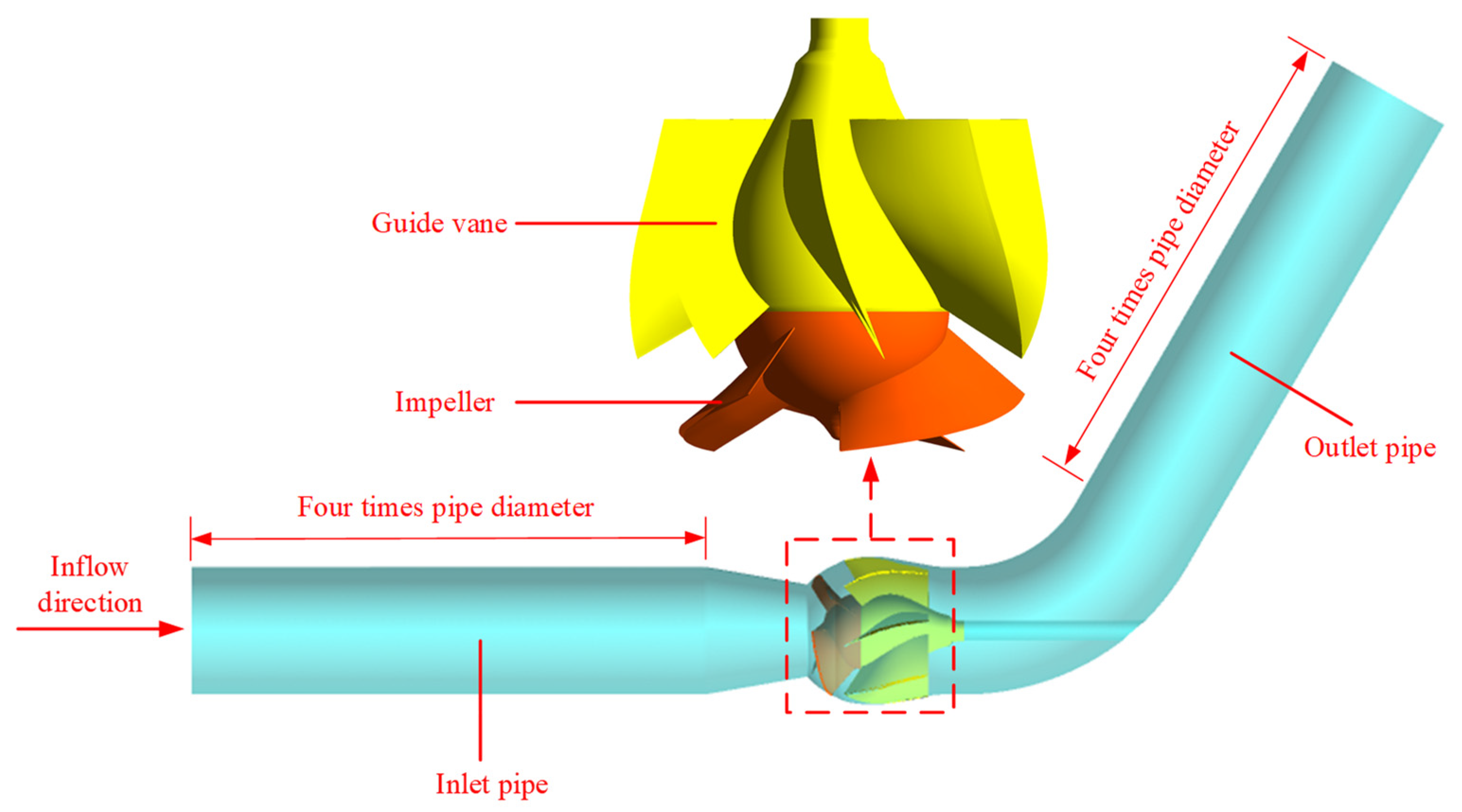
4.1. Energy Performance Analysis

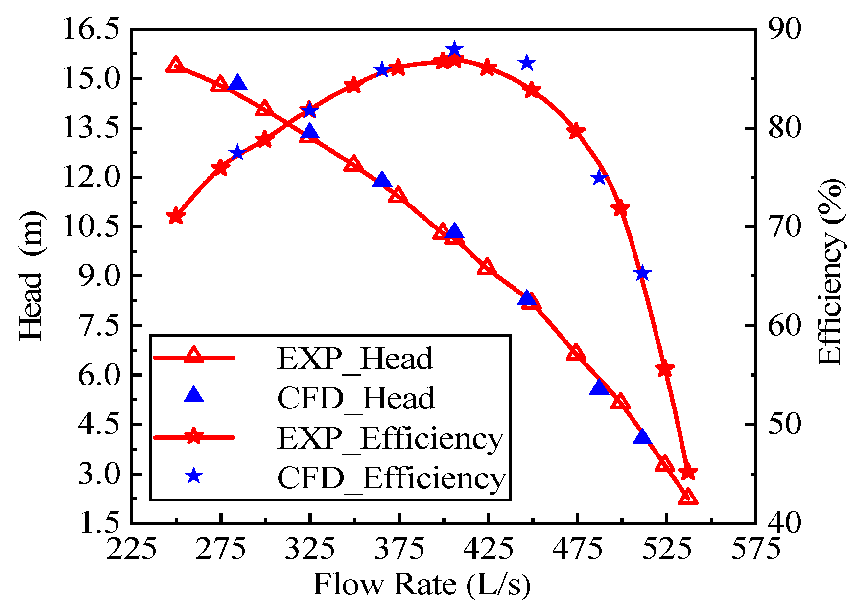
Figure 7 presents the external characteristic curves for the seven design schemes. Figure 7a shows that for a single blade deviation, the flow rate of the optimal hydraulic efficiency point of the mixed-flow pump gradually increased when blade No. 2 rotated from −4° to +4° (Design Schemes I–V). This result occurred because the flow capacity in the impeller passage generally tended toward larger flow rates with increases in the rotation angle. In all the design schemes, when the rotation angle of each blade was adjusted to 0° (Design Scheme III), the optimal hydraulic efficiency of the mixed-flow pump reached a maximum value. Therefore, it was concluded that BRADs changed the flow field and decreased the optimal hydraulic efficiency.

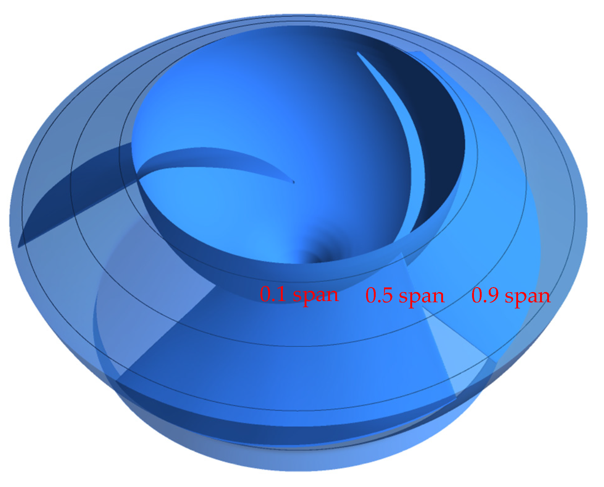
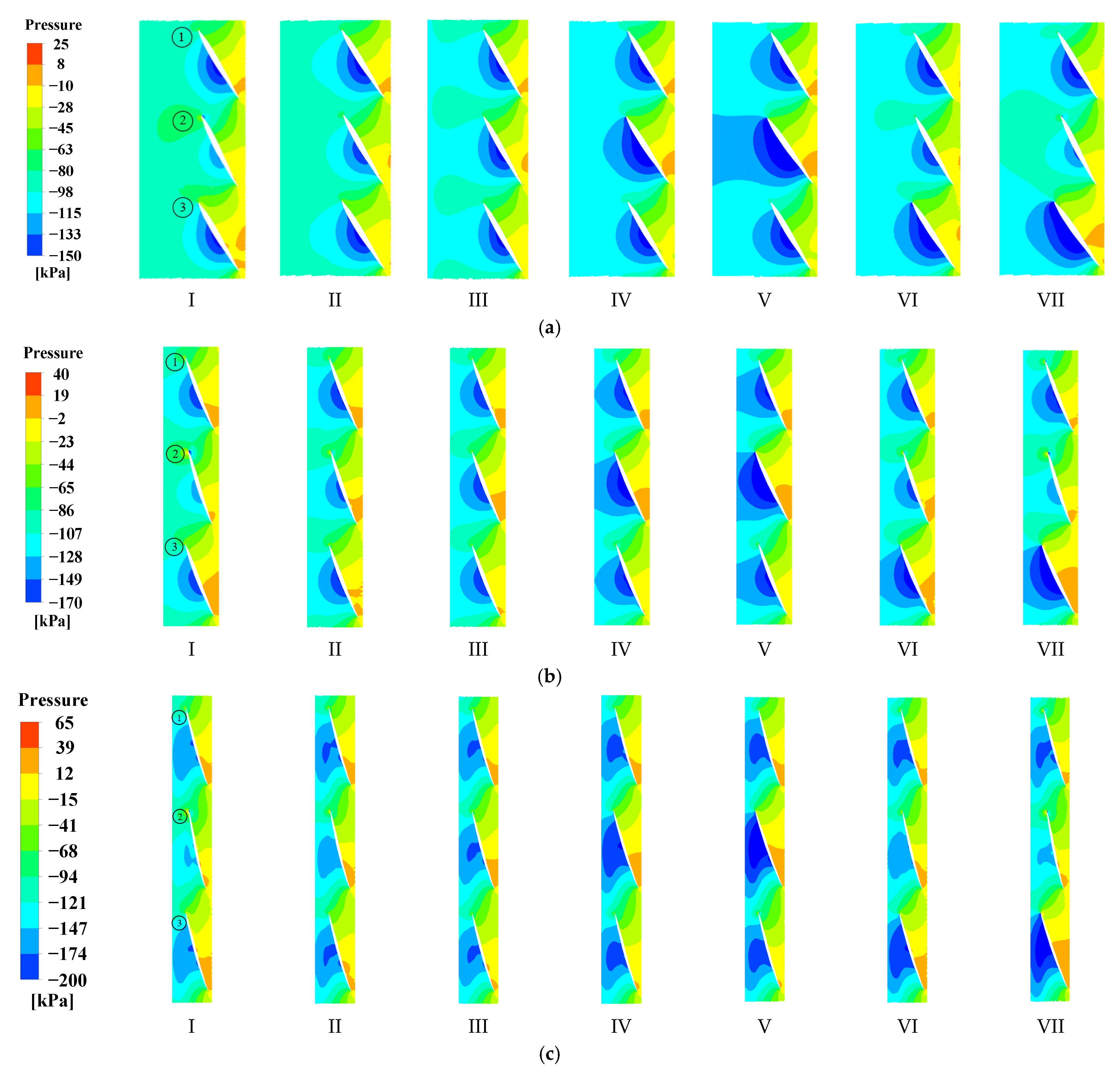
When the rotation angles of the other blades remained at 0° and the flow rate remained constant, the head of the mixed-flow pump gradually increased when blade No. 2 rotated counterclockwise from −4° to +4°, as shown in Figure 7b. Figure 8 and Figure 9 show the pressure distribution of each span in the impeller domain under the design flow rate, which can explain the curve rules described previously. The meaning of span is as shown in Equation (4). When there were no BRADs, the pressure distributions near the three blades were relatively centrally symmetrical, and the pressure gradients were distributed evenly. As blade No. 2 gradually deviated counterclockwise, the area of low pressure on the suction surface of the impeller gradually increased, while the pressure distribution on the pressure surface changed slightly. As a result, when the rotation angle of the blade deviated in a counterclockwise direction, the pressure difference between the pressure and suction surfaces of the impeller gradually increased. Therefore, the working capability of the impeller was gradually enhanced, and the head of the mixed-flow pump increased. When two blades deviated in opposite directions simultaneously (Design Schemes VI–VII), the working capacities of the blades canceled each other out, so the head curves did not change significantly.

$$\mathrm{span}=\frac{r-r_{\mathrm{hub}}}{r_{\mathrm{shroud}}-r_{\mathrm{hub}}}$$

(4)

In Equation (4), r is the radius at the span, r_hub is the hub radius of the impeller outlet, and r_shroud is the shroud radius of the impeller outlet.

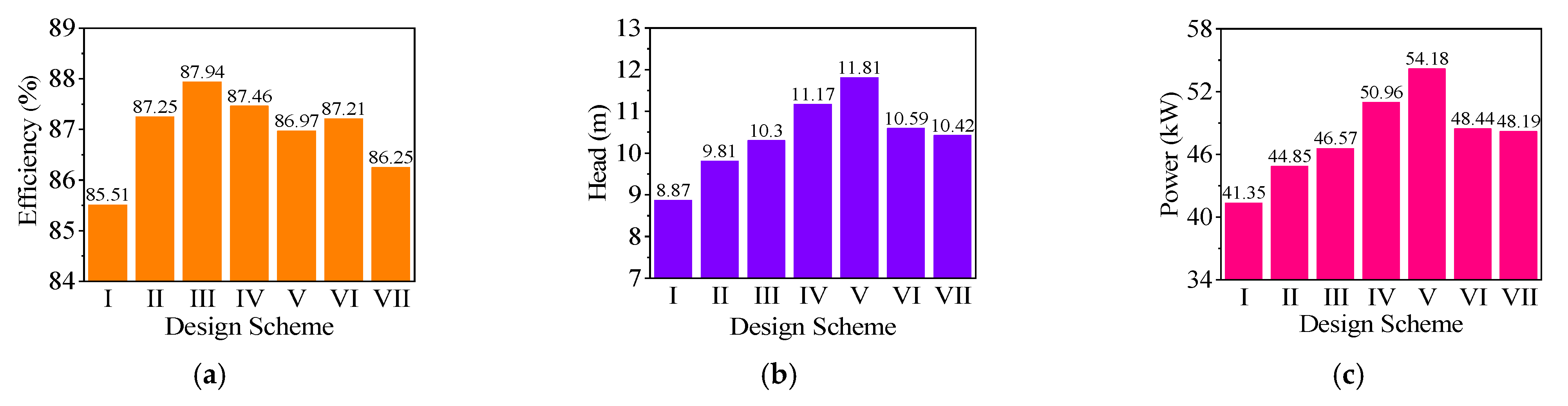
Figure 10 depicts comparisons of the energy performance of the mixed-flow pump for the different design schemes under the design flow rate. Figure 10a shows that the hydraulic efficiency point for each deviation scheme was reduced from that of Design Scheme III. When the rotation angle of the blade deviated clockwise (Design Scheme I–II), the pumping capacity of the impeller decreased. The optimal hydraulic efficiency corresponded to the condition of a small flow rate, so the hydraulic efficiency decreased. When the rotation angle of the blade deviated counterclockwise (Design Scheme IV–V), the power of the impeller increased. However, hydraulic efficiency is inversely proportional to power. As the power increased, the hydraulic efficiency decreased. When the two blades had opposite deviations (Design Scheme VI–VII), the force on the impeller was uneven, which caused more hydraulic losses and reduced hydraulic efficiency. The most significant reduction occurred for Design Scheme I, which had a decrease of 2.43%, followed by that for Design Scheme VII. Greater counterclockwise and clockwise blade deviations led to lower efficiencies. Figure 10b shows that when the blade deviation angle gradually increased from −4° to +4°, the head rose, and the gradient changed regularly. The head of Design Scheme V was 1.51 m higher than that of Design Scheme III. The head when two blades deviated in opposite directions was slightly higher than that when the blades had no deviations. Additionally, the head of Design Scheme VII was slightly lower than that of Design Scheme VI, perhaps because the fluid distribution in the pump was more uneven, thus causing more flow loss. The power was proportional to the head. When the head increased, so did the power. Therefore, the trend in Figure 10c was essentially the same as that in Figure 10b.

4.2. Pressure Fluctuation Characteristics

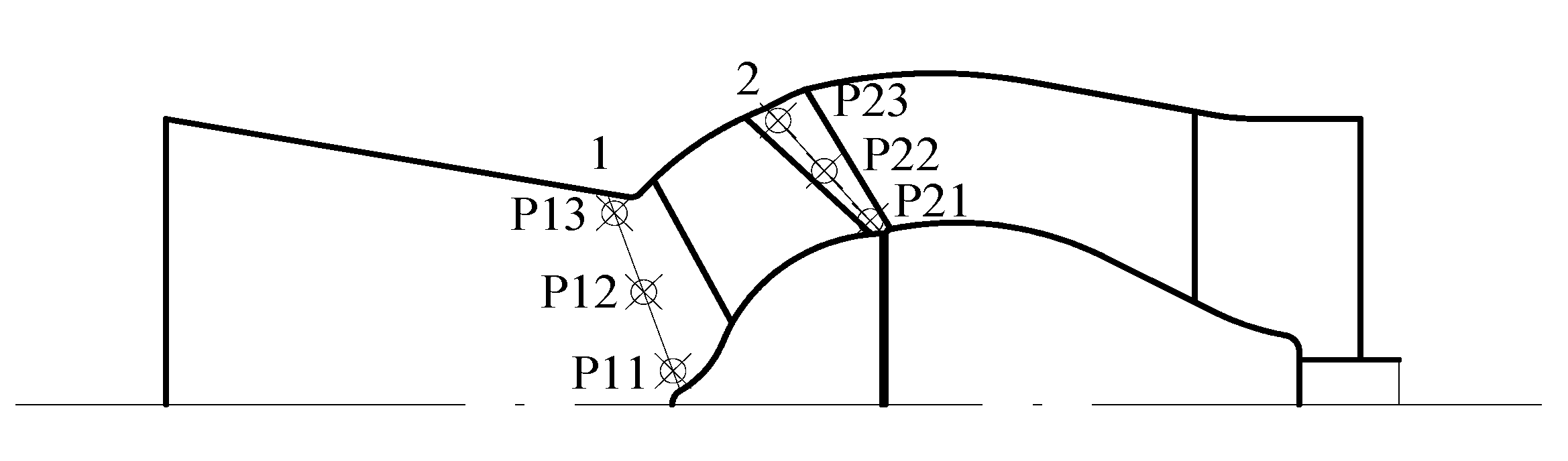
To study the variation trends of the pressure pulsation at different sections under the design flow rate, three monitoring points were set at the impeller inlet and outlet, named P11–P13 and P21–P23, respectively. Their locations are shown in Figure 11. Pij represents the positions of the monitoring points, where i = 1–2 represents the axial position from the inlet to the outlet of the pump, and j = 1–3 represents the radial position from the hub to the shroud.

The pressure coefficient, C_p, was selected to reflect the pressure fluctuation characteristics, and its relational expression is as follows [26]:

$$C_p=\frac{P_{\mathrm{i}}{-P}_{\mathrm{ave}}}{0{.5\rho u}^2}$$

(5)

In Equation (5), P_i represents the instantaneous pressure at the monitoring point, P_ave is the average pressure, ρ is the density of water, and u is the circumferential velocity at the outlet of the impeller.

4.2.1. Impeller Inlet

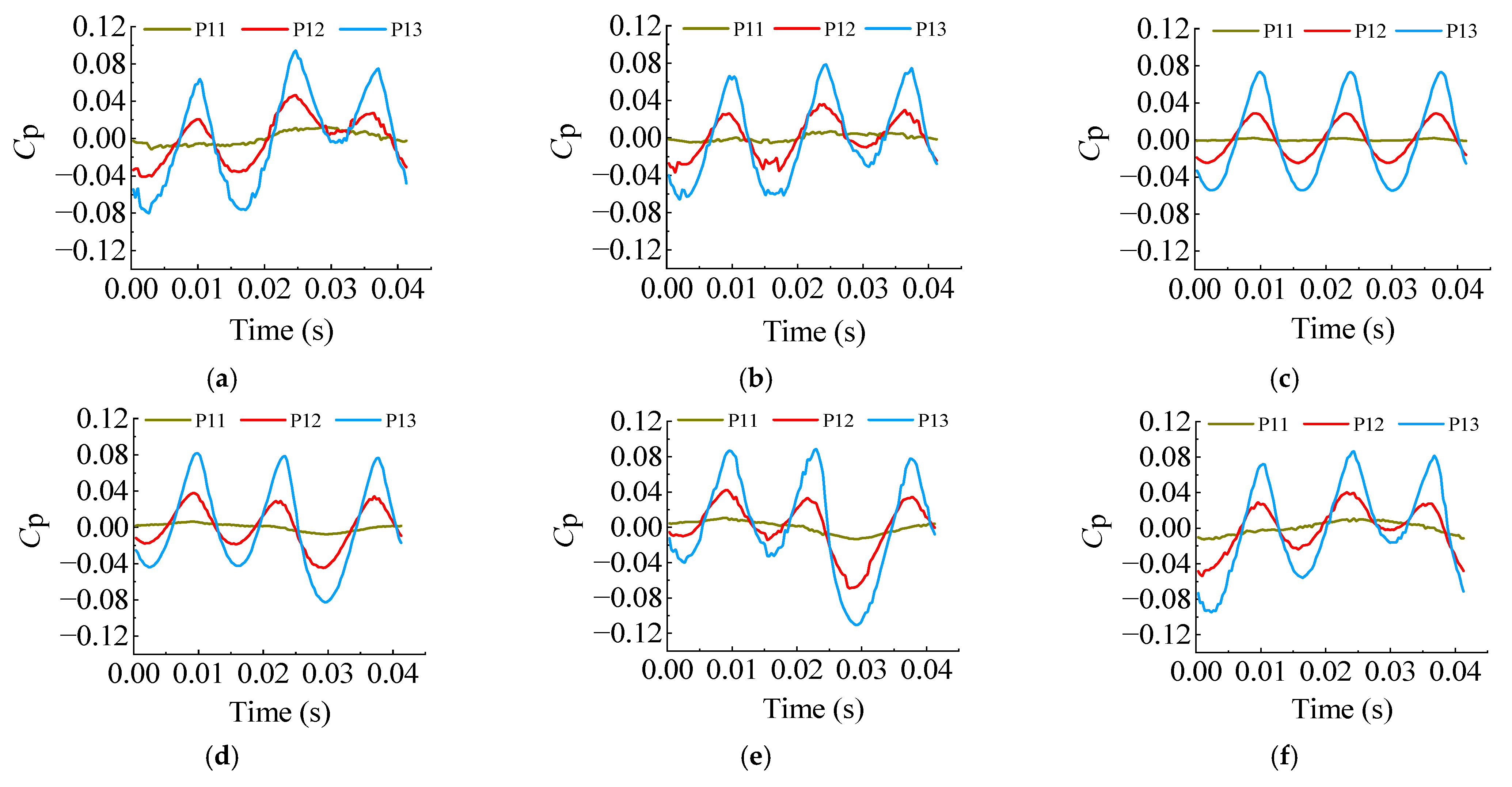
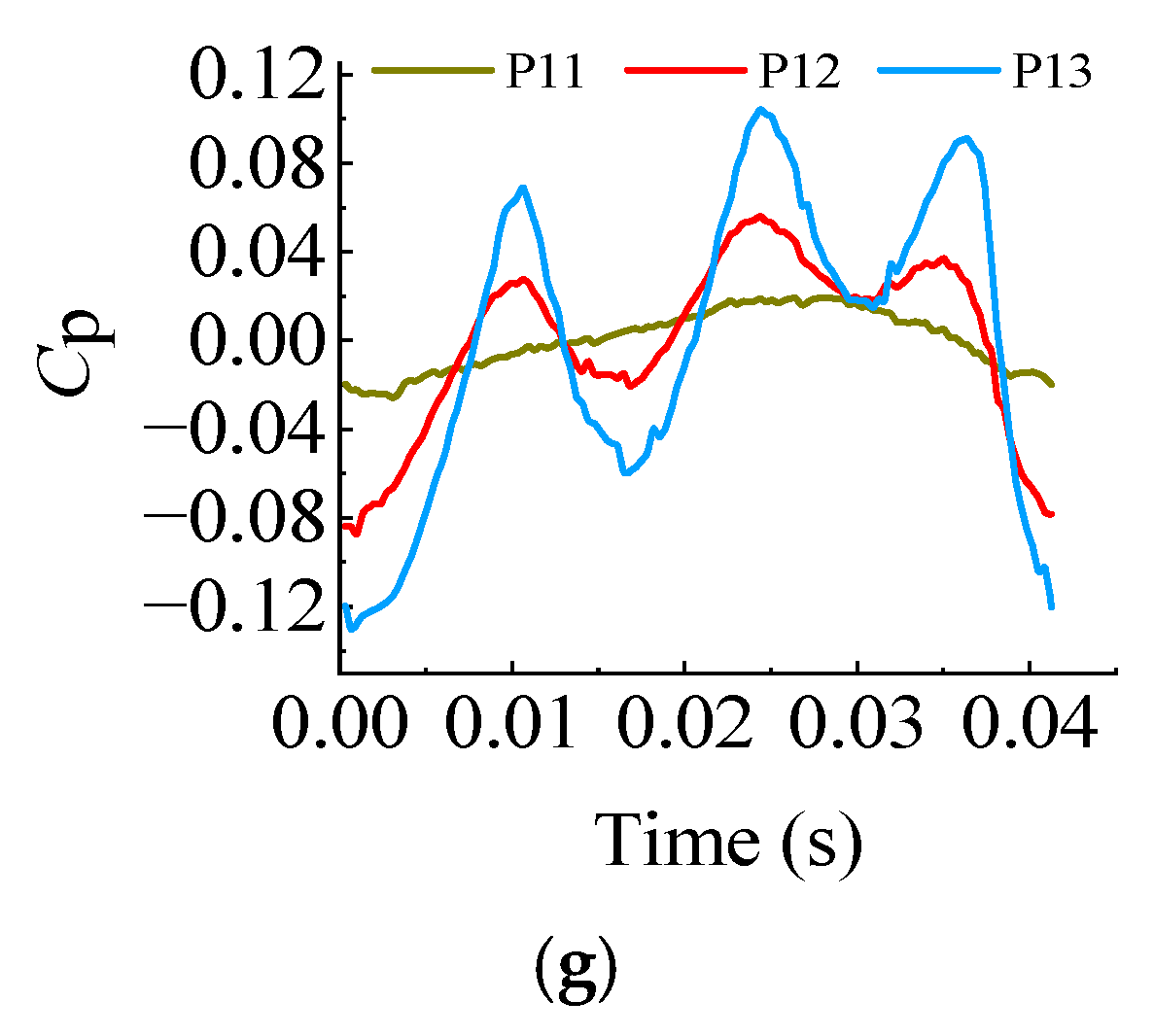
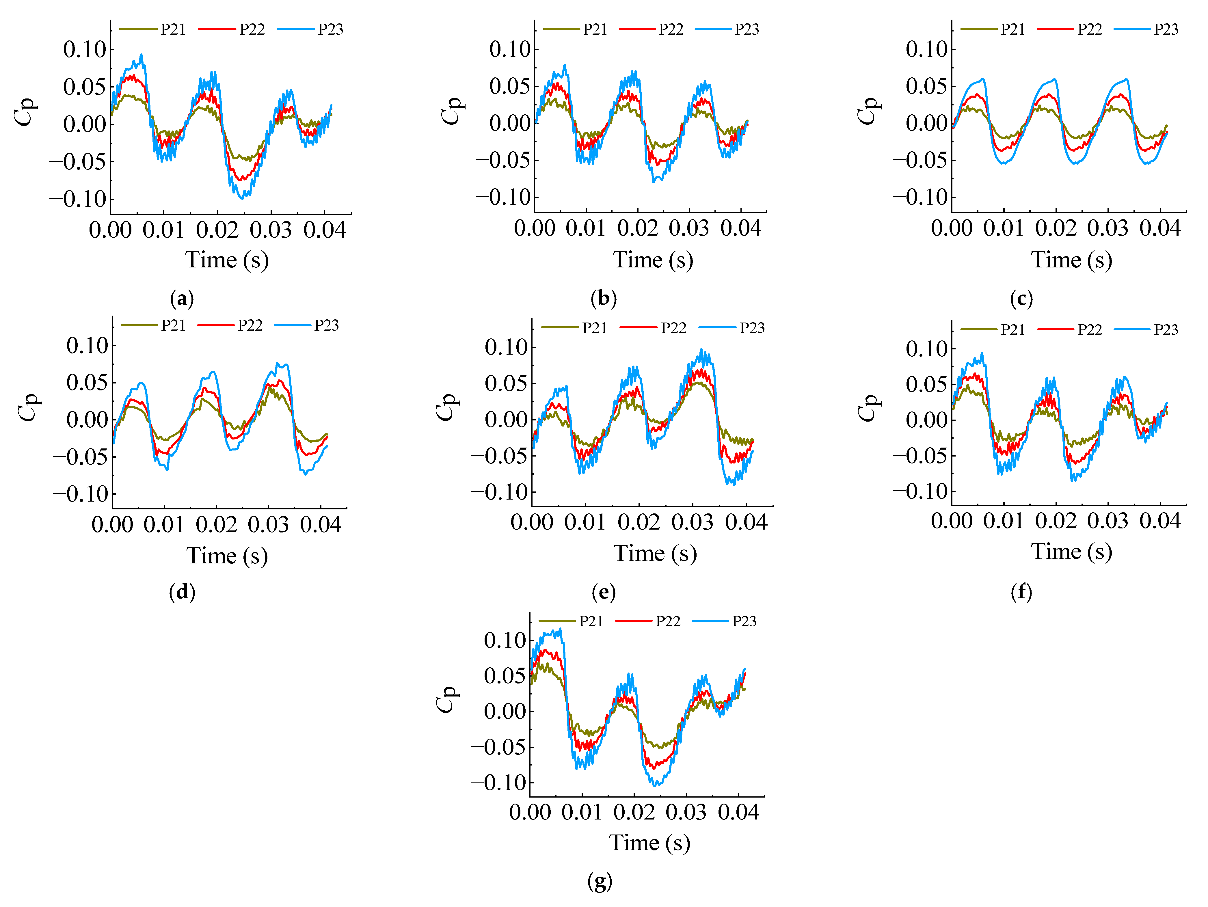
Figure 12 shows the time-domain variations of the impeller inlet pressure fluctuations for each design scheme under the design flow rate. The last rotation period of the impeller was selected for analysis. In Design Scheme III, which had no BRADs, the impeller regularly passed through the monitoring points three times every rotation period. Therefore, the pressure distribution around the hub side, the middle position, and the shroud side presented three sets of very regular peaks and valleys, and the number of peaks was equal to the number of impeller blades. In other design schemes, although there were three peaks and valleys near the shroud side and the middle position, the periodic curves near the hub side were not obvious. These results show that when the blade rotation angle deviated, the pressure fluctuations near the hub side of the impeller inlet monitoring point were less affected by the rotation of the blade, and that the fluid flow was disordered. When there was a deviation of a single blade (Design Schemes I, II, IV, and V), the peak values for the three blades at P12 and P13 changed little compared to the changes for Design Scheme III. However, the minimum value for one set of blades decreased with increases in the blade rotation angle and increased with decreases in the blade rotation angle. This result indicates that the central symmetry of the pressure distribution at the impeller inlet was destroyed, which primarily affected the fluctuation values in the valleys. When two blades deviated, the pressure coefficient in one valley for Design Scheme VII was higher than that for Design Scheme VI, and another was lower.

Table 2. Pulsation amplitudes at P1.

Monitoring Point	Design Scheme
	I	II	III	IV	V	VI	VII
P11	0.02383	0.01239	0.00016	0.01409	0.02422	0.02324	0.04514
P12	0.08722	0.07304	0.05368	0.08273	0.1114	0.09365	0.14325
P13	0.1731	0.14364	0.12818	0.16467	0.19924	0.18056	0.23519

displays the pressure coefficient pulsation amplitudes for the last rotation period in each design scheme. The values for all the deviation design schemes were higher than those for the scheme without deviation, and the most obvious increase occurred for Design Scheme VII. These results indicate that when BRADs occurred, the pressure fluctuation range at the impeller inlet increased.

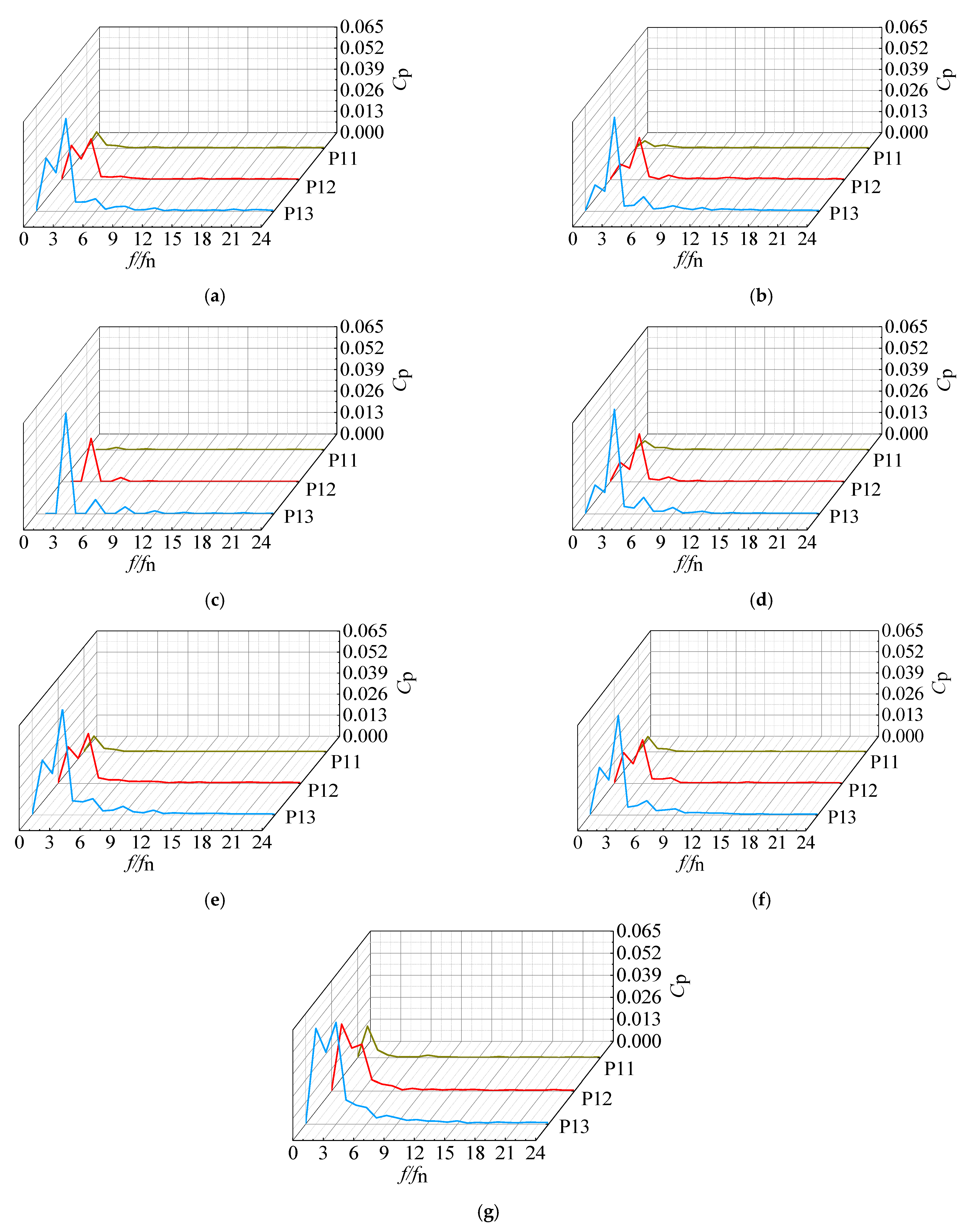
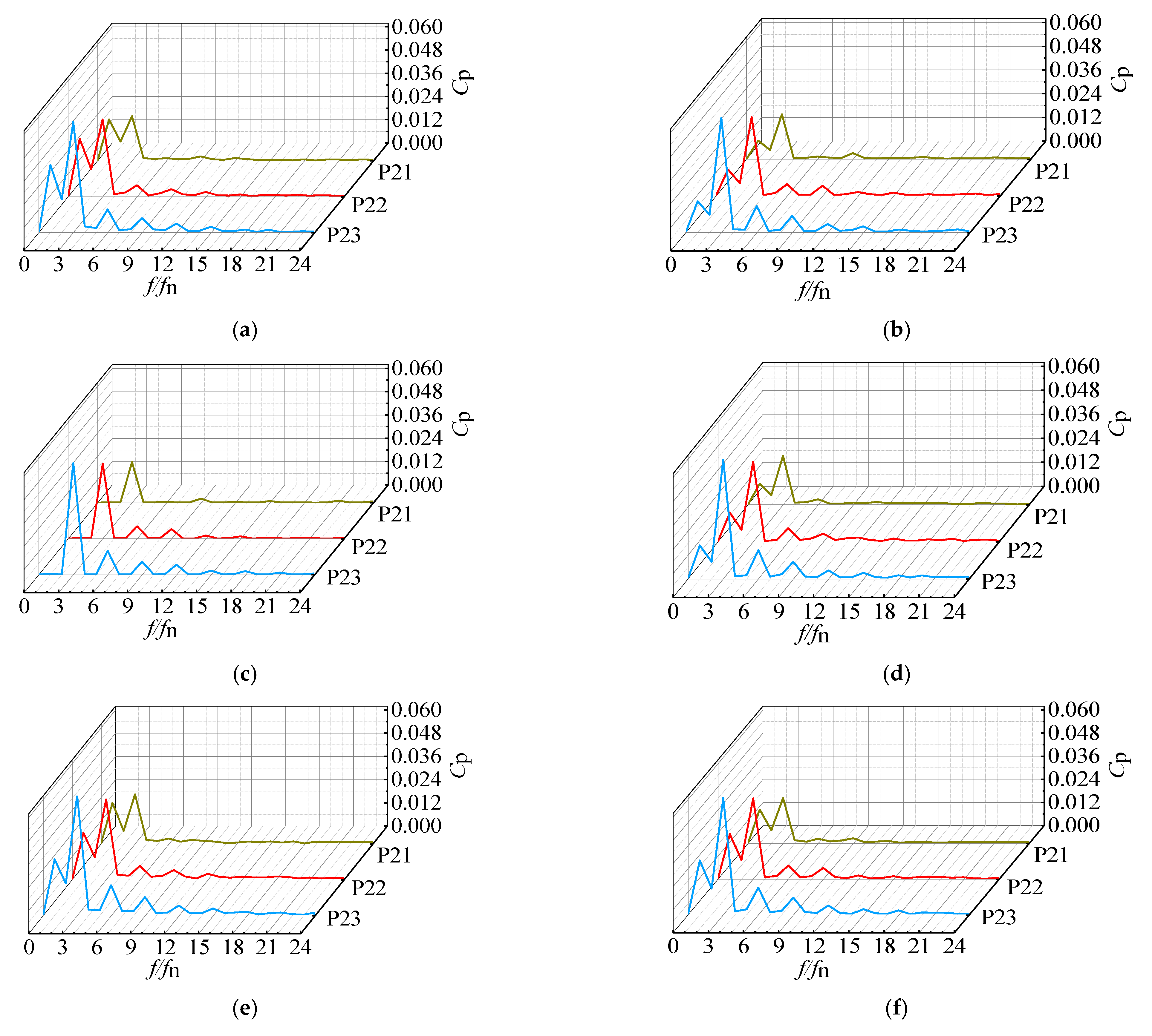
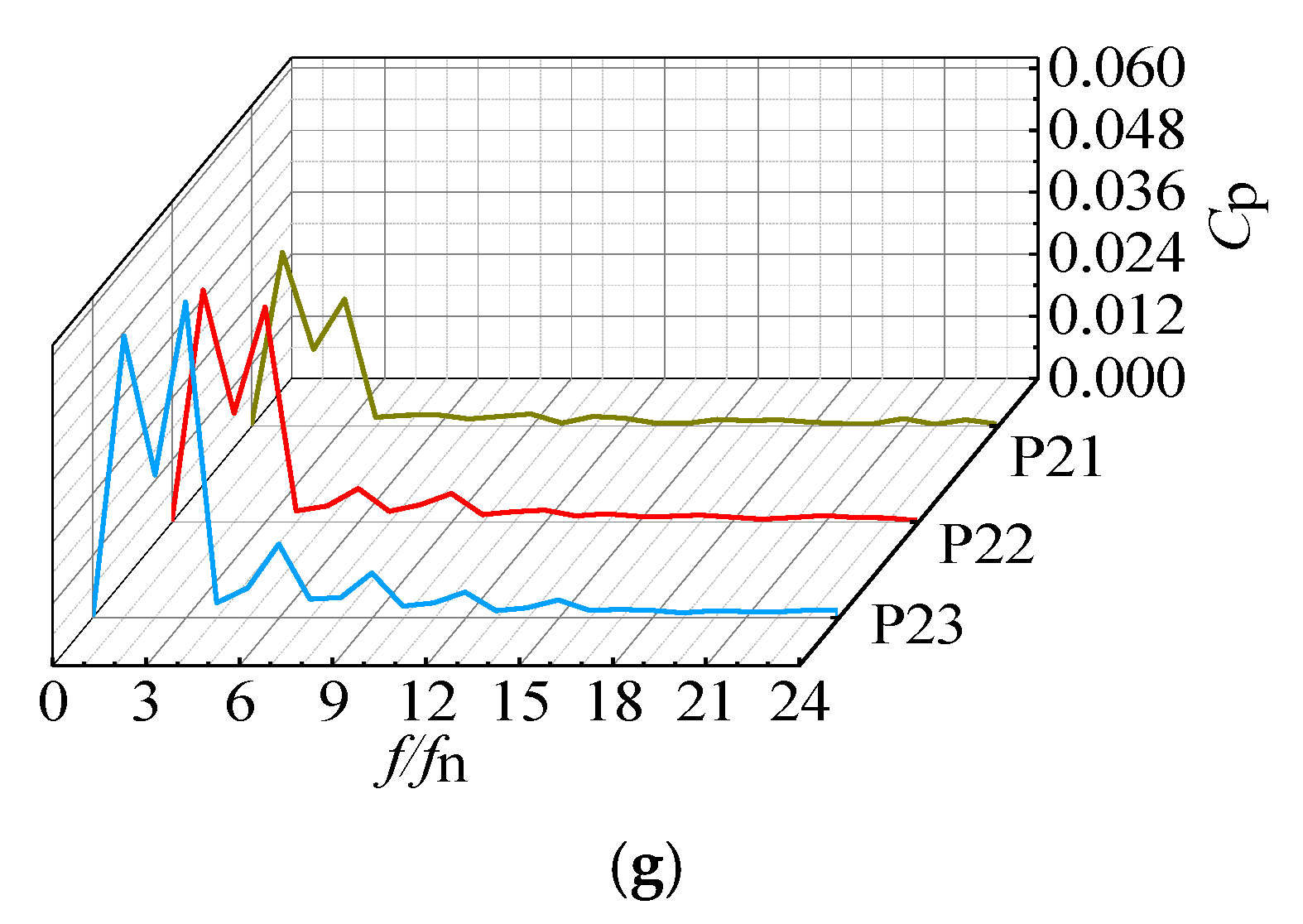
The calculated time-domain data were converted into frequency-domain data by a fast Fourier transform (FFT) to obtain the frequency distribution of the pressure signal. The shaft frequency was f_n = n/60 = 24.17 Hz, and the horizontal axis of the frequency-domain diagram was set as multiples of the shaft frequency. Figure 13 depicts the frequency-domain diagrams of the pressure pulsations at the impeller inlet for different design schemes. In all the schemes, the amplitude of the dominant pressure pulsation frequency increased gradually from the hub side to the shroud side. Unlike Design Scheme III, which had no BRADs, the dominant pressure pulsation frequency at P11 changed to the shaft frequency for the other schemes, and large secondary frequency amplitudes appeared at P12 and P13. This result may have occurred because BRADs caused the velocity distributions at the hub side to be uneven, resulting in increases in vorticity and changes in hydraulic excitation. This type of deviation had the greatest influence on Design Scheme VII because the dominant pressure pulsation frequency at the middle position became the shaft frequency, and a secondary frequency corresponding to the amplitude of the dominant frequency emerged on the side of the shroud.

Table 3. Amplitudes of the dominant frequency at P1.

Monitoring Point	Design Scheme
	I	II	III	IV	V	VI	VII
P11	0.00984	0.00441	0.00122	0.0053	0.00965	0.00928	0.01849
P12	0.02502	0.02589	0.02621	0.02894	0.03053	0.02669	0.03911
P13	0.05703	0.05781	0.06102	0.06328	0.06558	0.06124	0.0596

shows the amplitude of the dominant frequency at the impeller inlet for each design scheme. At P11, the amplitude changed significantly, and the amplitudes for Design Schemes I, II, IV, V, VI, and VII were 8.07, 3.61, 4.34, 7.91, 7.61, and 15.16 times that of Design Scheme III, respectively. For a single blade deviation, the amplitudes of the dominant frequency pulsations at P12 and P13 increased with a counterclockwise deviation. Deviations of two blades in opposite directions led to extremely uneven distributions of the impeller inlet pressure and significant increases in the amplitude.

4.2.2. Impeller Outlet

Figure 14 shows the time-domain variations in the impeller outlet pressure fluctuations for each design scheme. The impeller outlet results had more tortuous curves than did the results for the impeller inlet. This occurred because BRADs caused differences in speed and direction in each blade passage, leading to violent collisions between the high-speed water at the outlets. Due to the rotor-and-stator interference of the impeller and guide vane, there were three distinct peaks and valleys in the last rotation period.

Table 4. Pulsation amplitudes at P2.

Monitoring Point	Design Scheme
	I	II	III	IV	V	VI	VII
P21	0.0888	0.06744	0.04482	0.0752	0.08856	0.08735	0.11956
P22	0.14074	0.11161	0.07684	0.10176	0.12945	0.12709	0.16713
P23	0.19268	0.15911	0.11463	0.15084	0.18779	0.18121	0.22127

lists the pulsation amplitudes of the pressure coefficient at the impeller outlet for each design scheme. The occurrence of BRADs increased the pulsation amplitude of the pressure coefficient at the impeller outlet, and the range of the pressure change increased.

Figure 15 presents the frequency-domain diagrams of the pressure coefficient at the impeller outlet for all design schemes. The amplitude of the dominant pressure fluctuation frequency increased gradually from the hub side to the shroud side in all design schemes. When there were no BRADs, the dominant and secondary pressure pulsation frequencies were equal to the blade frequency and multiples of the blade frequency, respectively. When there were BRADs, the dominant pressure pulsation frequencies at each monitoring point for Design Schemes I, II, IV, V, and VI remained unchanged and equal to the blade frequency, but the secondary frequency changed to the shaft frequency. These results show that, despite the deviations in the blade rotation angle, the blade frequency was still dominant at the impeller outlet. However, the secondary frequency cannot be ignored, and greater BRAD led to a greater rise in the amplitude. Design Scheme VII had the most significant influence on the pressure pulsations at the impeller outlet because the dominant frequencies near the hub side and middle position were converted into the shaft frequency, while a secondary frequency with a larger amplitude appeared near the shroud side. In this case, the entire pump operation remained in a low-frequency pulsation state, which can cause resonance of the pump.

Table 5. Amplitude of the dominant frequency at P2.

Monitoring Point	Design Scheme
	I	II	III	IV	V	VI	VII
P21	0.02296	0.02272	0.0209	0.02428	0.02555	0.02341	0.03354
P22	0.03982	0.03979	0.03856	0.04003	0.04146	0.04182	0.04473
P23	0.05887	0.05805	0.05747	0.0596	0.06226	0.0607	0.06095

shows that BRADs increased the amplitude of the dominant pressure pulsation frequency at each monitoring point, which was different from the situation at the inlet. These results occurred because the P2 monitoring points were located behind the impeller, and the asymmetric outflow in the three blade passages had high velocities. Therefore, the collision was greater and more severe than for Design Scheme III. The dominant pressure pulsation frequencies near the shroud side were not affected by BRADs (all of them were equal to blade frequencies). At P23, the dominant pressure pulsation frequencies of Design Schemes I, II, IV, V, VI, and VII were 1.021, 1.01, 1.037, 1.083, 1.056, and 1.061 times that of Design Scheme III, respectively.

4.3. Force on the Impeller

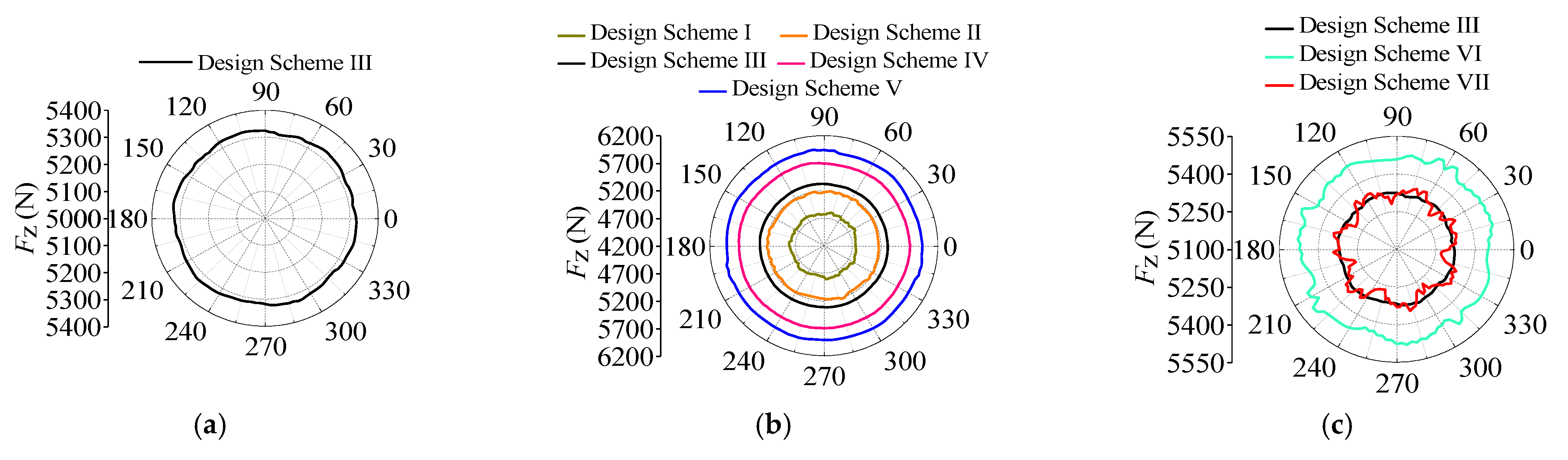
When the mixed-flow pump was running, the rotation of the impeller generated axial lift on the fluid, and the fluid produced an equal and opposite axial force on the impeller. Figure 16 depicts the trajectory distribution of the axial force in the last rotation period under the condition of 1.0 Q_des. The curves are essentially closed, indicating that the axial force of the impeller reached a stable state. The fluctuation of axial force is defined as the difference between the maximum value and the minimum value of axial force in the last period. The axial force fluctuated little with the rotation of the pump, and the entire trajectory was approximately circular. Figure 16b shows that when a BRAD occurred for a single blade, the total axial force on the impeller increased with increases in the blade rotation angle and decreased with decreases in the rotation angle. This result occurred because the axial force was determined by the pressure on the blade surface. In Figure 9, the pressure difference on the blade surface increased with increases in the blade rotation angle, resulting in increases in the axial force, and vice versa. The fluctuation values of axial force for design schemes I, II, III, IV, V, VI, and VII are 75.05 N, 68.76 N, 16.59 N, 36.02 N, 66.68 N, 64.08 N, and 89.75 N, respectively. When two blades deviated in opposite directions, the fluctuations in the axial force increased sharply, indicating that the axial force stability was poor.

Table 6. Average axial forces.

Flow Rate	Design Scheme
	I	II	III	IV	V	VI	VII
0.8 Qdes	6247.73	6515.96	6567.58	6831.19	6967.51	6667.69	6552.88
1.0 Qdes	4778.09	5172.14	5320.67	5698.87	5917.74	5465.83	5316.03
1.2 Qdes	2663.05	3265.04	3576.19	4103.41	4456.4	3779.95	3530.11

presents the average axial force on the impeller at flow rates of 0.8 Q_des, 1.0 Q_des, and 1.2 Q_des. When the flow rate increased, the axial force decreased in each scheme. For the 1.0 Q_des flow rate, the average axial forces of Design Schemes I, II, IV, V, VI, and VII were 0.898, 0.972, 1.071, 1.112, 1.027, and 0.999 times that of Design Scheme III, respectively. When the deviation directions of two blades were opposite each other, the axial force of the impeller was essentially the same as that when there were no deviations (Design Scheme III). The results show that when two blades deviated symmetrically and reversely, the axial forces of the blades canceled each other out, leading to a situation similar to that in the scheme without deviations.

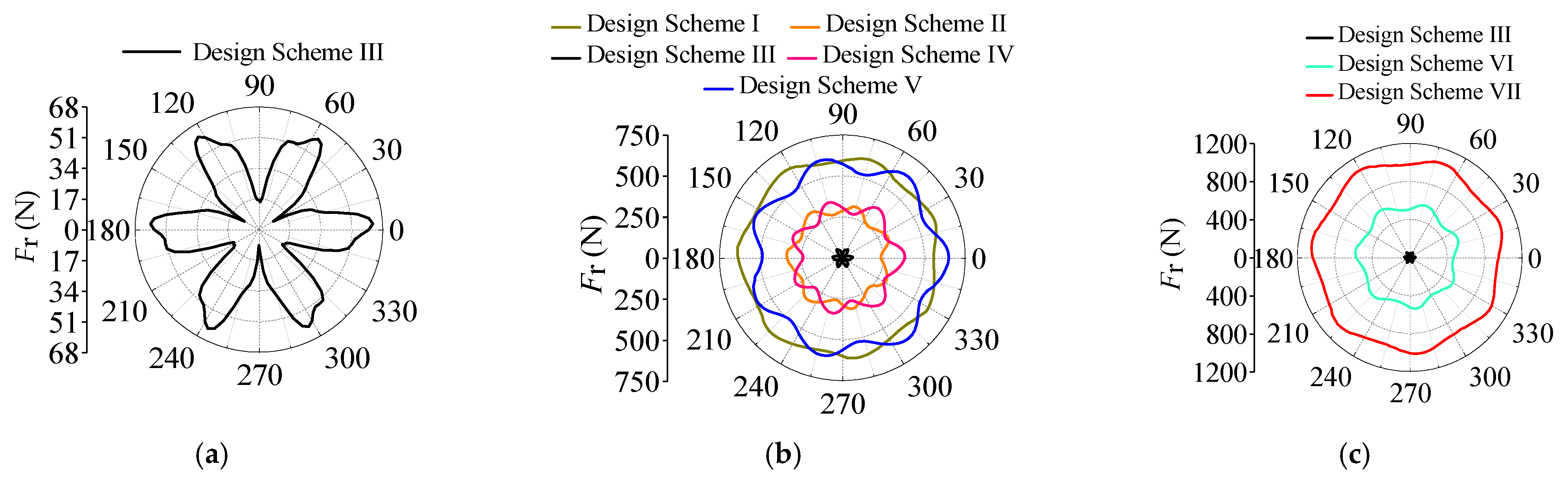
Figure 17 shows the trajectory distributions of the radial force on the impeller in the last rotation period under the condition of 1.0 Q_des. When there were no deviations, the radial force fluctuated periodically with six lobes, which was twice the number of impeller blades. The force center was essentially located at the center of the circle, indicating that the radial force of the impeller was stable and the torque of the pump shaft was relatively balanced. When BRADs existed, each design scheme presented seven obvious peaks and valleys. This result occurred because as the impeller passed through seven guide vane blades within one rotation period, the radial force changed seven times periodically. 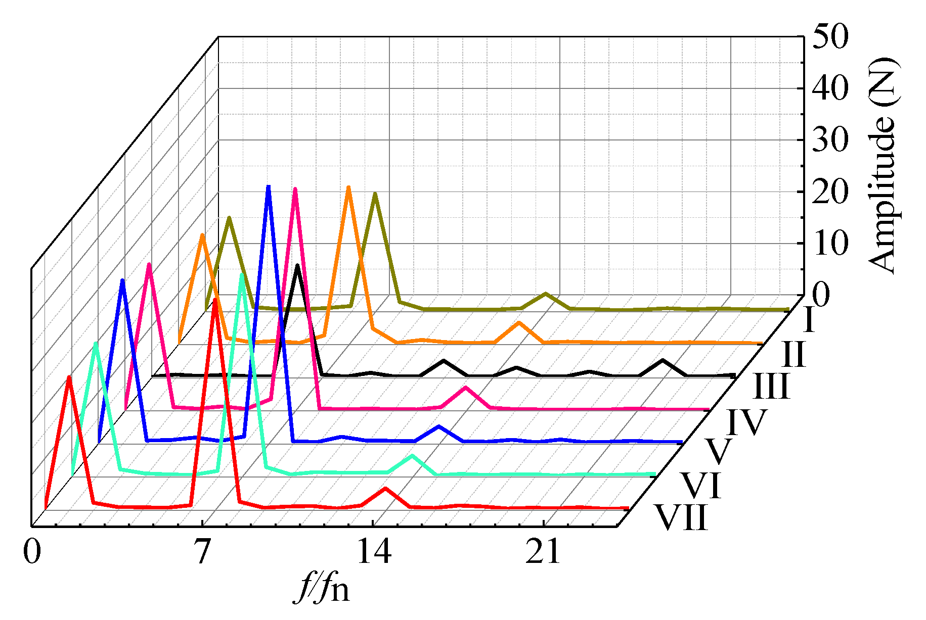Figure 18 shows that the dominant frequencies of the radial force on the impeller for the design schemes with deviations were different from those of the design scheme without BRADs and that they were related to the number of guide vane blades. When BRADs occurred, the amplitude of the dominant pulsation frequency was larger than that when there were no deviations, which could cause the torque of the pump shaft to be unstable.

Table 7. Average radial forces.

Flow Rate	Design Scheme
	I	II	III	IV	V	VI	VII
0.8 Qdes	508.20	243.20	40.00	278.18	508.58	452.97	869.93
1.0 Qdes	597.91	289.70	39.48	309.91	568.28	518.49	993.22
1.2 Qdes	684.16	340.07	29.27	368.32	702.65	612.63	1198.93

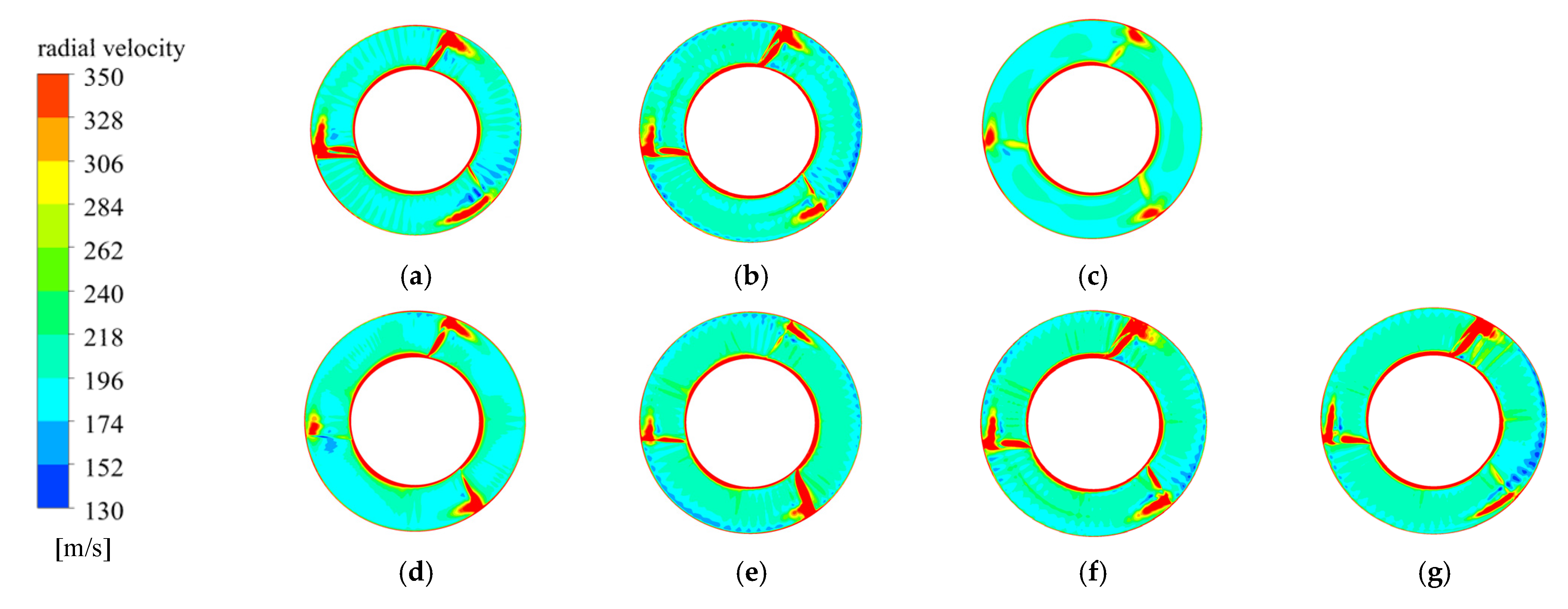
presents the average radial force on the impeller at flow rates of 0.8 Q_des, 1.0 Q_des, and 1.2 Q_des. In the absence of angle deviations, the radial force decreased with increases in the flow rate. However, the radial force increased with increases in the flow rate when there were angle deviations. For the condition of 1.0 Q_des, the average radial forces of Design Schemes I, II, IV, V, VI, and VII were 15.14, 7.34, 7.85, 14.39, 13.13, and 25.16 times that of Design Scheme III, respectively. In the radial velocity nephogram shown in Figure 19, the area of radial high-speed zone under the condition of blade angle deviation is obviously larger than that under the condition of no deviation (design scheme III), which may cause an increase in the radial force of the impeller. These results show that the radial force increased dramatically when BRADs occurred. When the rotation angles of two blades were in opposite directions, the radial force generated on the impeller reached a maximum. Therefore, the occurrence of BRADs enhanced the resultant radial force on the impeller, which would lead to more serious swing and deformation of the pump shaft, thereby causing a certain degree of pump instability and shortening its service life.

5. Conclusions

In this study, the energy performance, pressure pulsation characteristics, and axial and radial impeller forces were analyzed under BRAD conditions using numerical simulations. Three primary conclusions can be drawn:

(1)

The BRAD phenomenon decreased the optimal hydraulic efficiency and destroyed the central symmetry of the low-pressure area near the suction surface of the impeller. When a single blade deviated, the hydraulic efficiency and head curves moved toward larger flow rates as the rotation angle deviated counterclockwise, and vice versa.

(2)

Influenced by BRADs, the pressure coefficient at the minimum point of the valley of a deviated blade decreased with increases in the blade rotation angle at the impeller inlet. The dominant pressure pulsation frequencies remained unchanged (and were equal to the blade frequency) near the shroud side at the inlet and outlet of the impeller. The maximum amplitude and the dominant pressure pulsation frequency both increased with increases in the absolute value of the BRAD near the hub side of the impeller inlet and the shroud side of the impeller outlet. The amplitudes of the dominant pressure pulsation frequencies of Design Schemes I, II, IV, V, VI, and VII near the hub side at the impeller inlet were 8.07, 3.61, 4.34, 7.91, 7.61, and 15.16 times that of Design Scheme III (without BRADs), respectively. Additionally, the amplitudes of the dominant pressure pulsation frequencies of Design Schemes I, II, IV, V, VI, and VII near the shroud side at the impeller outlet were 1.021, 1.01, 1.037, 1.083, 1.056, and 1.061 times that of Design Scheme III, respectively.

(3)

When the BRAD was counterclockwise, both the axial and radial forces increased. The radial force of the impeller was increased by at least six times from that when there were no BRADs, and the dominant radial force pulsation frequency changed to the blade frequency of the guide vane.

BRADs reduced the optimal hydraulic efficiency of the water pump and caused low-frequency pulsation and unstable impeller force. Therefore, the research results can provide a basis for the fault diagnosis of mixed-flow pumps operation.