Article

An Integrated Scheme of the Data-Driven Multi-Block FCMs for Modeling the Steady Turning Motion of Motorboats

1
Navigation College, Dalian Maritime University, Dalian 116026, China
2
School of Science, Dalian Maritime University, Dalian 116026, China
3
The Faculty of Electronic Information and Electrical Engineering, School of Control Science and Engineering, Dalian University of Technology, Dalian 116024, China
*
Author to whom correspondence should be addressed.
J. Mar. Sci. Eng. 2023, 11(2), 442; https://doi.org/10.3390/jmse11020442
Submission received: 15 December 2022 / Revised: 8 February 2023 / Accepted: 14 February 2023 / Published: 17 February 2023
(This article belongs to the Section Ocean Engineering)

Abstract

:
The steady turning motion of merchant ships is modeled according to industry specifications. However, challenges arise when motorboats are modeled. This study proposes a novel data-driven multi-block fuzzy cognitive map (FCM) model trained based on sea trials with four ship states. The optimal positions sampled by two different types of sensors were modeled using inverse variance weighting, which takes both Cartesian coordinate transformation and the constraints of the locations of the apparatuses into consideration. Combining these samplings with a scheme of multi-block FCMs, we conducted a study on data from motorboat trials. Our results closely approximate the data from motorboat trials at sea and are validated by a generated dataset of the classical model. Furthermore, we reveal the characteristics of our scheme, including the number of data blocks, the boundary of each block, and the parameters of the FCM for each block. As opposed to the classical method, the proposed scheme is insensitive to speed. This study presents a promising step toward mining modeling information from ship trials.

1. Introduction

Motorboats are divided into several categories according to their usage, including, but not limited to, lifeboats used for survivors, yachts for entertainment, and unmanned surface vessels (USVs) for scientific research. Determining how to steer efficiently is crucial to navigation safety, environmental protection, and research on autonomous ships, which are closely related to the productivity and livelihood of various stakeholders.
The steady turning motion of a vessel can influence movement performance [1]. These parameters are printed in the wheelhouse poster, which is posted in a conspicuous space on the bridge for officers or pilots [2]. Many alternative methods are available for the modeling schemes of vessels, such as the mechanism model, computational fluid dynamics (CFD), and the identification model. However, the actual effectiveness of these solutions in nautical practice and their applications still deserve further study.
In the last decade, the mechanism model, represented by the Abkowitz [3] model or the maneuvering mathematical modeling group model (MMG) [4], has provided a standard solution to this problem for the shipping industry [5]. For example, the mechanism model is used to perform a quick check for ship design to determine whether the ship meets the IMO criteria [6]. This is a framework used to investigate a mathematical model for a ship maneuvering simulator, such as the ship–ship interaction related to restricted water areas [7]. Furthermore, it is also a means of verifying the effectiveness of the numerical [8] method or system identification method [9]. One of the mechanism model’s core technologies is obtaining the hydrodynamic derivatives for a mathematical model of ship maneuvering motion. These can be obtained using captive model tests [7], system identification techniques applied to free-running model test results [10], or numerical computations [8]. However, this model depends on towing tanks with a certain amount of investment. Few institutions worldwide can meet the needs of basic research. These constraints make modeling the movement of motorboats difficult.
The CFD scheme was successfully applied for form-changeable boats [11], the dynamic behaviors of drifting ships [12], a high-speed planning boat [13], and flying boat planing [14]. Meanwhile, there have been many research achievements in the applciation of combinations of CFD and mechanism model methods. Sukas et al. used a URANS approach to obtain hydrodynamic derivatives and then implemented them in an MMG model for a twin-propeller/twin-rudder ship [15]. Sakamoto et al. proposed a similar CFD-MMG approach [16]. However, the computational burden of this scheme is heavy due to the large computational grid. Moreover, the verification data limit its application in engineering.
The identification scheme is another important method. Abkowitz [17] identified the Esso Osaka model with 59 parameters using an extended Kalman filter. However, some variables in this training set are easily disturbed during measurements, such as sway velocity and yaw rating. In addition, there are effects of drift parameters and dynamic cancelation. Subsequently, Källström et al. [18] used the pseudorandom binary sequence (PRBS) signal to excite the system, but this may reduce the safety of the ship in practice [19]. According to [20,21,22], the data in the model or full-scale tests can reduce this risk. There are other ways to cope with the nonlinearity of ship maneuvering motion. Bai et al. proposed using locally weighted learning to approximate the nonlinear function using segmented linear functions [23]. Ouyang et al. explored the use of Gaussian process regression optimized by a genetic algorithm [24], local Gaussian process regression [25], Gaussian process regression [26], and adaptive hybrid-kernel function-based Gaussian process regression [27] to conduct research on ship nonlinear motion modeling and obtained satisfactory results. However, these methods depend on the numerous states of ship movement. Some variables, such as sway speed or yaw rating, are easily disturbed by the external environment and are challenging to collect in practice. Therefore, these studies may be limited in practical application.
A classical scheme is used to identify the maneuvering indices of K and T in the Nomoto model [28]. When the Nomoto model is combined with the linear mathematical model of the ship [3], the linear hydrodynamic derivatives are estimated by Clarke’s regression formula [29] using seven parameters. We can then approximate the indices of K and T using these derivatives. However, this linear model applies to a small and medium rudder angle and is sensitive to speed. Perera et al. [30] proposed a modified nonlinear steering model to expand the range of working conditions. Subsequently, they performed a second-order Nomoto model with nonlinear constraints to design course-tracking based on stable conditions [31], but this still needs to be studied under unstable conditions. Due to the nonlinearity of the movements of vessels, building a model that fulfils the requirements of structural simplicity and functional generalization is challenging.
The neural network model is a black-box identification scheme. Moreira et al. [32] proposed a modeling method based on a time-delayed recurrent neural network. In [33,34], an approach was used that combined neural networks with other functions. Although these studies only rely on data, network structures have no any explanation in terms of semantics. In practice, we have observed such a phenomenon. Crewmembers who do not know any mathematical models still master their steering skills through more training, which indicates that such models still have room for improvement.
An identification scheme is also applied when modeling motorboats. Wang et al. [35] proposed the constrained multistep prediction (CMSP) method to identify a USV model with 32 parameters. However, the risk of the motorboat being driven by the PRBS excitation signal increases during the test. In [36], a USV model with four thrusters was identified using the normal equation. Although there were fluctuations between the truth values and the predictions, their study showed the potential significance of the data-driven model based on sea trials. Xiong et al. [37] realized the berthing task for a USV by using a real-time attitude meter and microwave radar sensors. However, there are few such sensors installed on-board. Furthermore, when the signal accuracies signals are low, ships may collide with the wharf due to the large inertia, which is consistent with the investigation in [38].
Based on previous research, full-scale or towing tank model tests require a high level of investment. Due to the high risk of operation and the necessity of sampling readily disturbed variables simultaneously, professional technicians are indispensable. Furthermore, these methods neglect the seafarers’ prior knowledge. Therefore, this study focused on building an FCM modeling framework based on a combination of the generalization utilization of data in nautical practice and the dominant acquaintance of officers.
An FCM is an intelligent soft computing method that combines fuzzy and neural networks [39,40]. Gao et al. [41] has theoretically proved the feasibility of modeling a steady turning motion. However, engineering applications have rarely been directly examined. First, the training data are derived from ship simulators without disturbances and any loss of sampling [42]. Second, the effect of projection transformation on safety has not yet been explored. Because coordinate transformation can affect the accuracy of positions on charts, it is necessary to verify practicability. Third, the work conditions of the sensors on-board were not checked. Therefore, it is important to design a data-driven modeling scheme based on fuzzy cognitive maps using measurements in nautical practice.
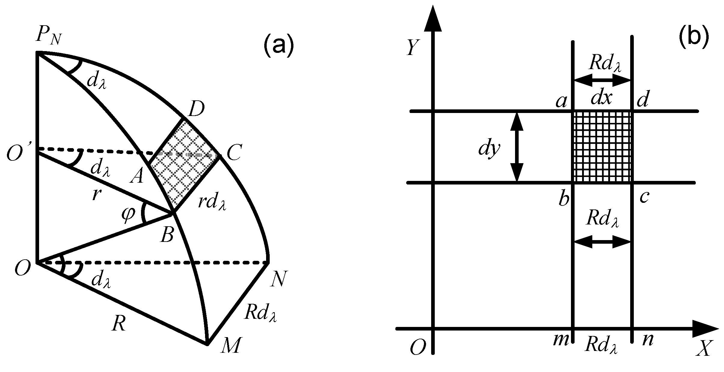
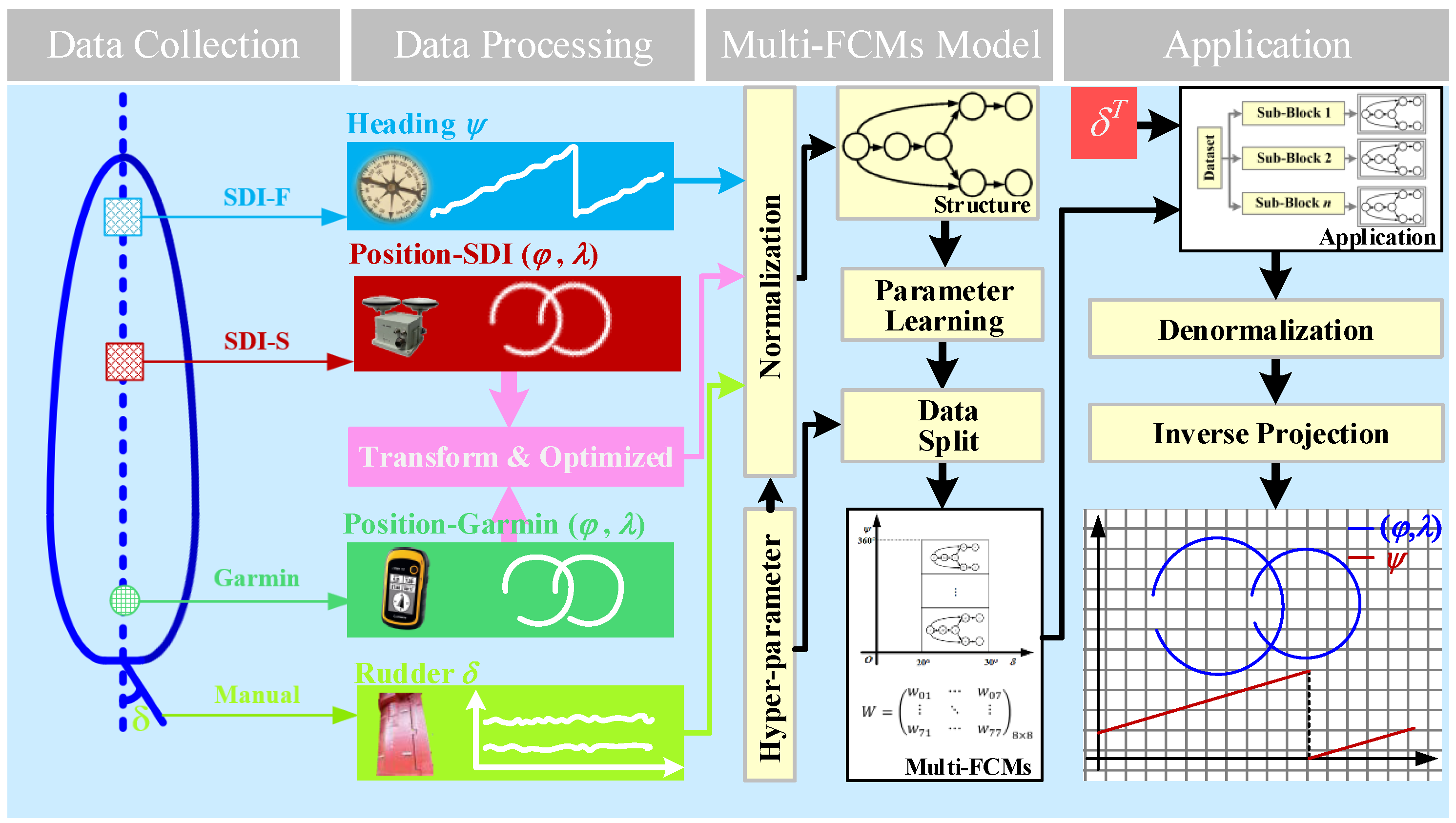
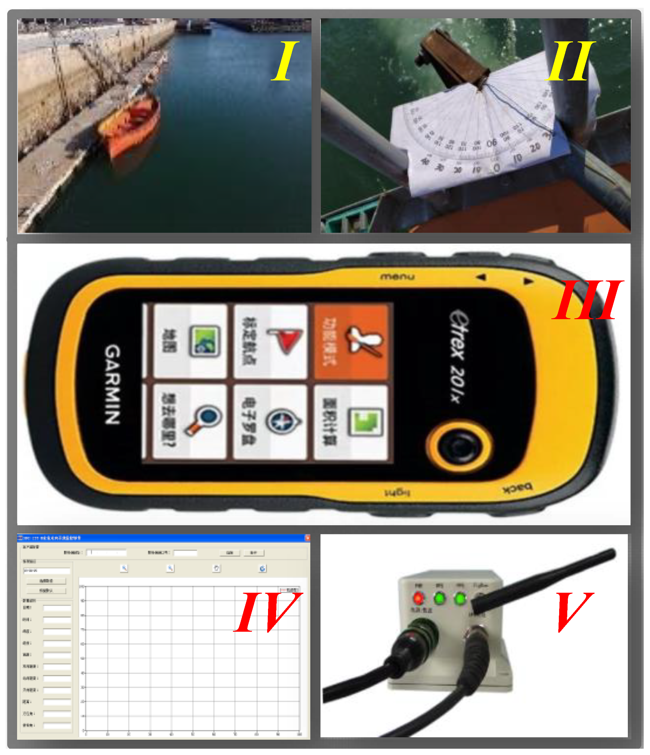
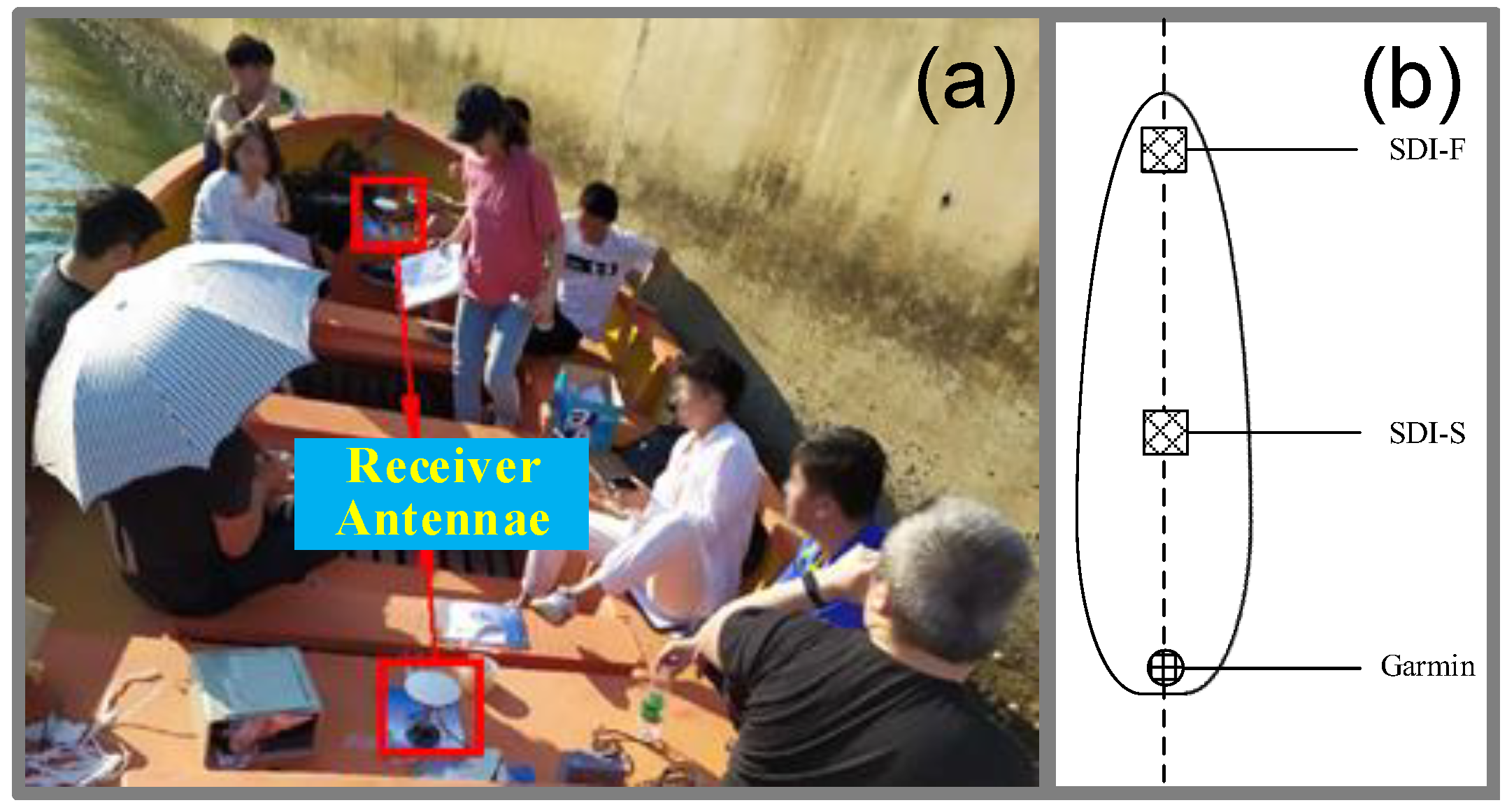
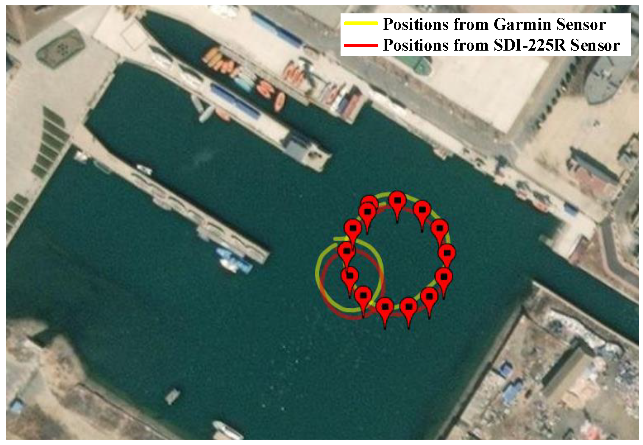
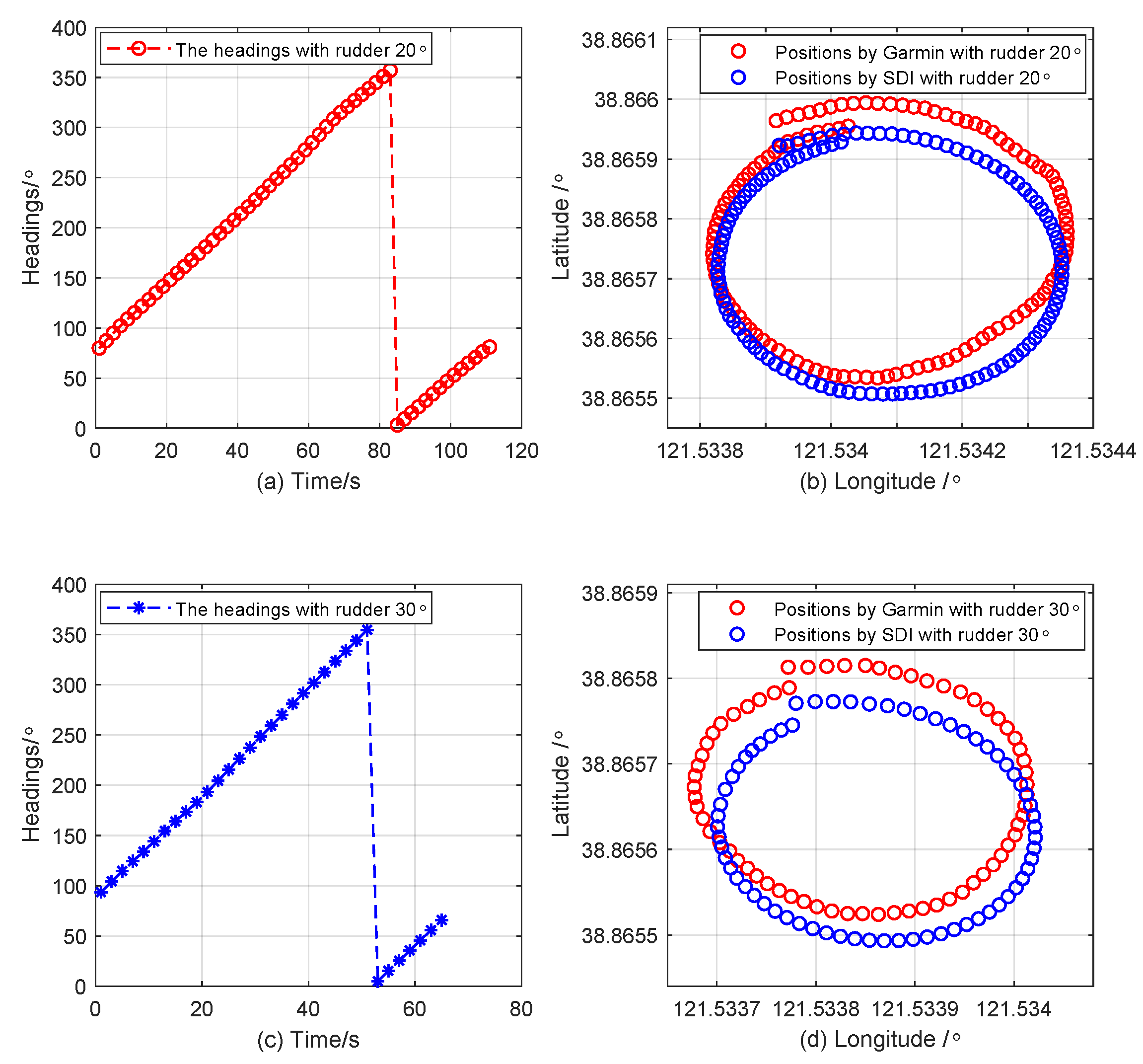
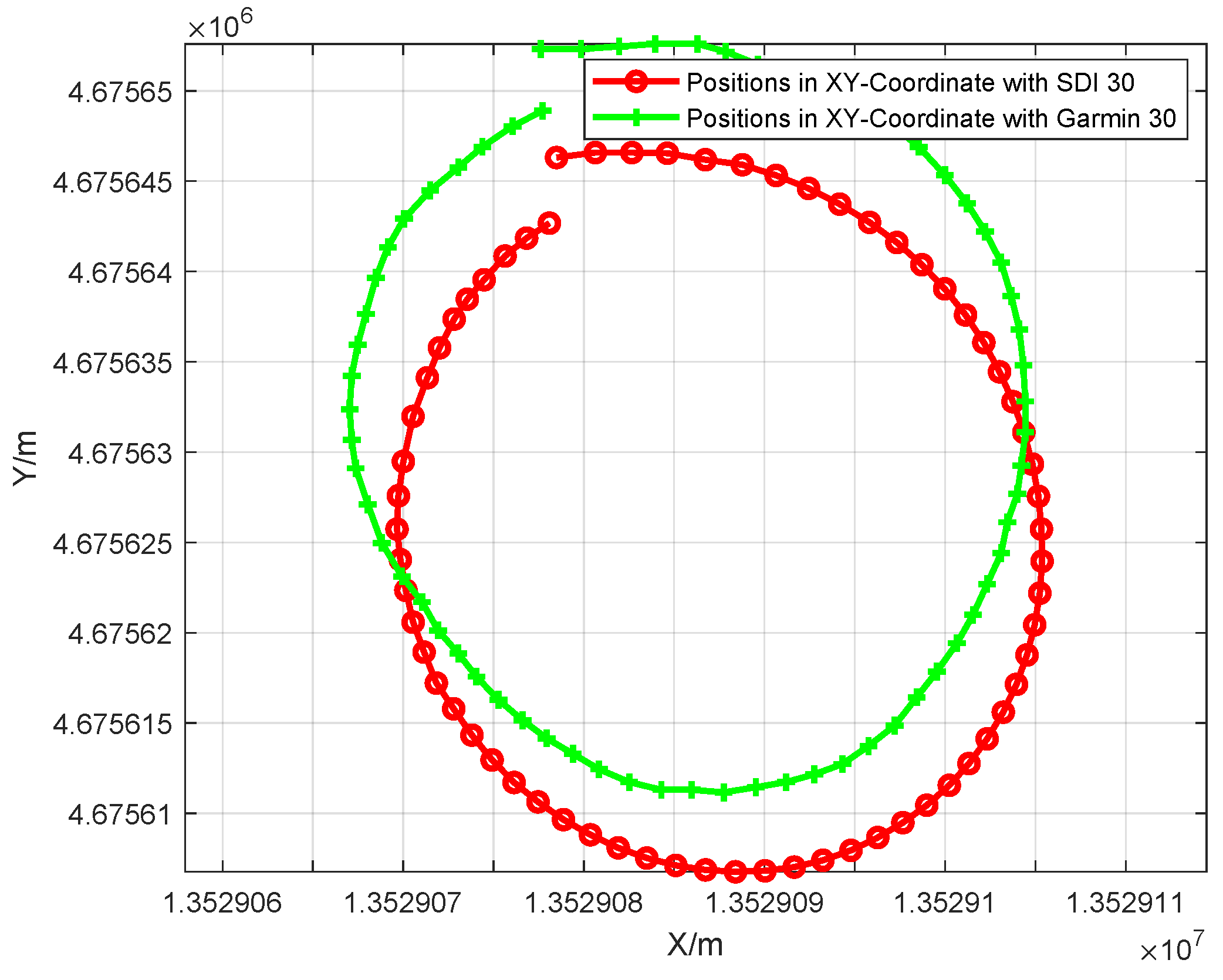
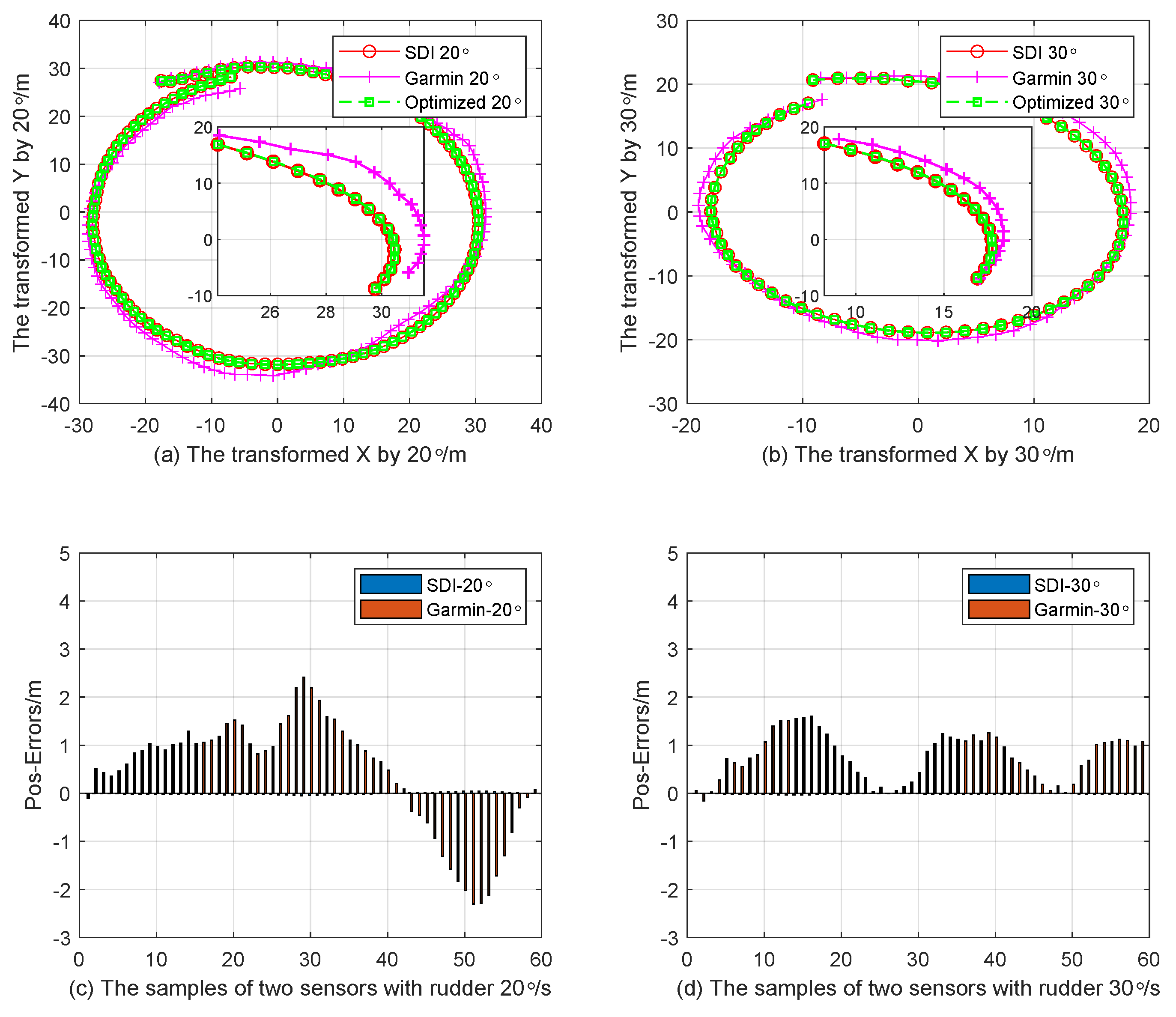
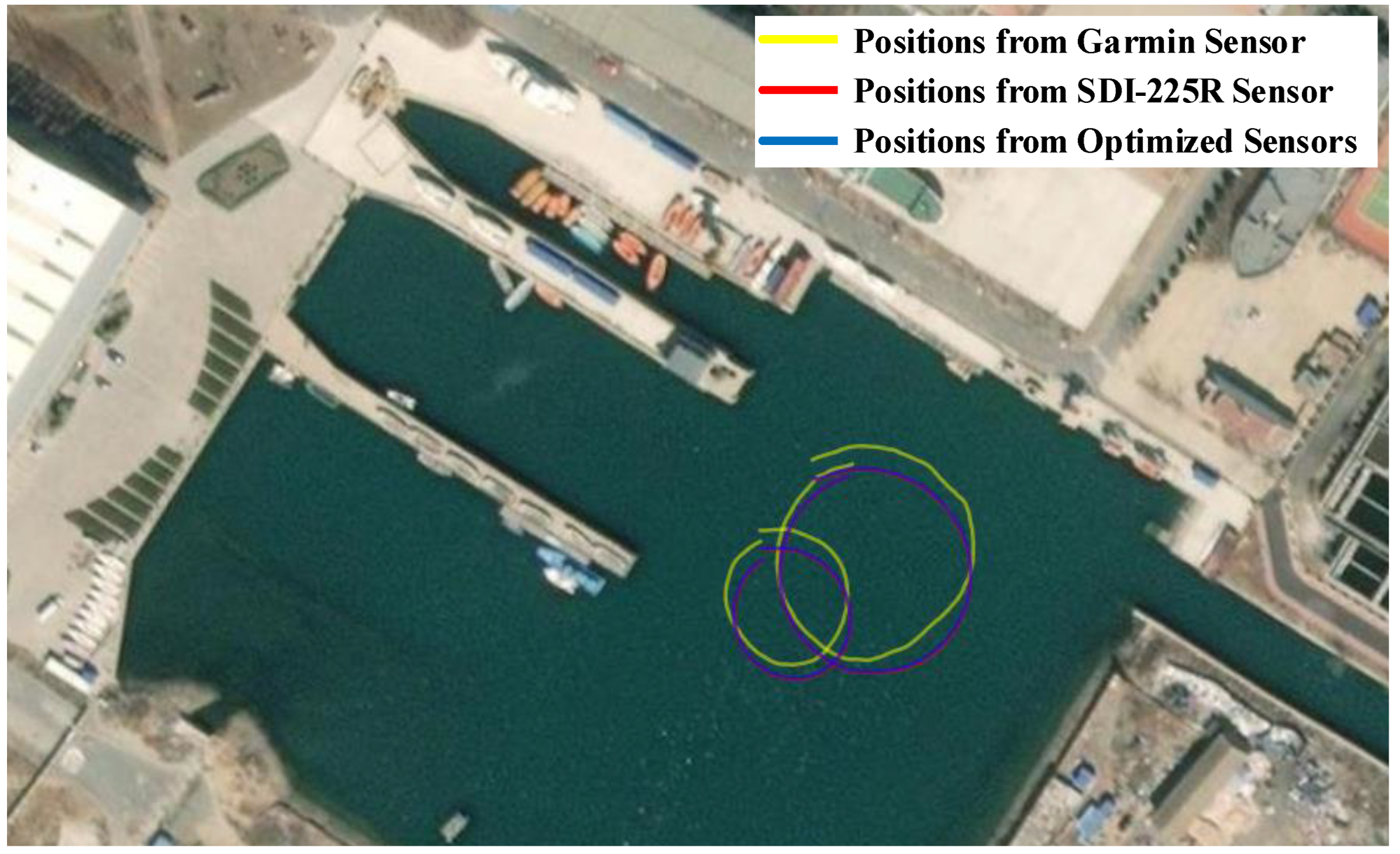
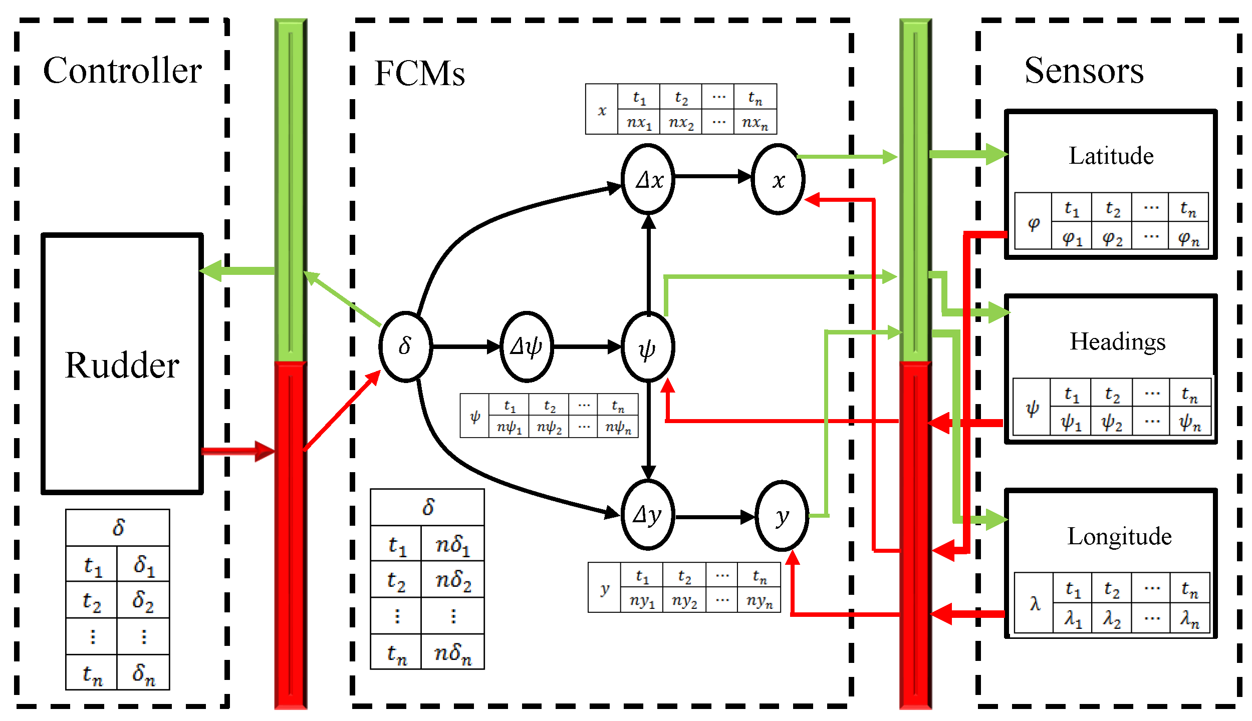
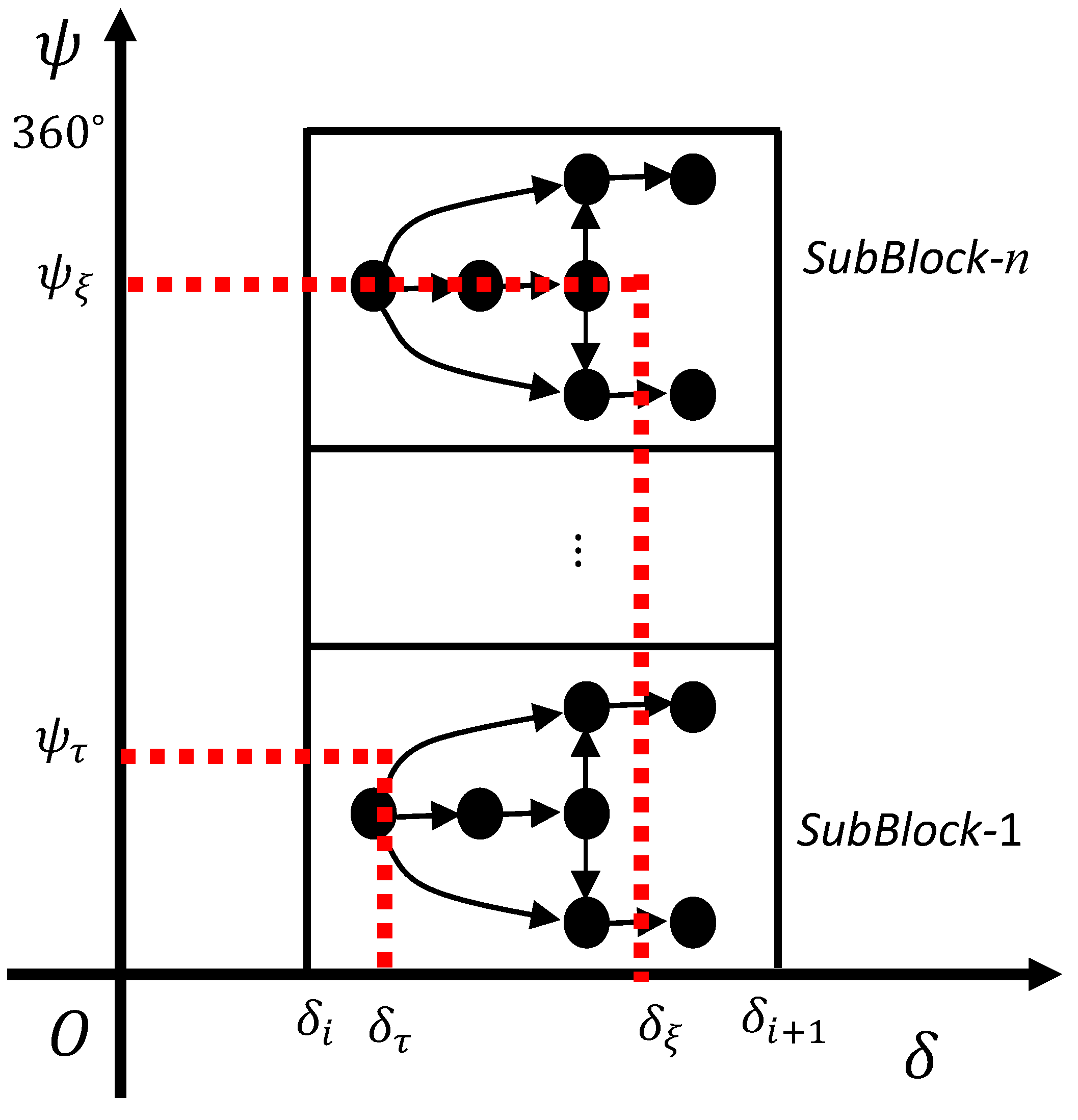
This study aimed to develop a practical framework to model a steady turning motion based on a data-driven multi-block FCMs model using motorboat sea trials. First, sea trials were organized to measure the states of motorboats using sensors. Subsequently, the positions sampled by the multi-source sensors were transformed to XY plane coordinates using Mercator projection, and the optimal positions were then estimated by inverse variance weighting. These sampled data were used to train the model of the multi-block FCMs according to the divide-and-conquer strategy. Finally, the experimental results indicate the effectiveness of the presented scheme. The contributions of the current work can be summarized as follows.
  • We organized sea trials to collect four states ( λ , φ , ψ , and δ ) of motorboats at sea and then combined the coordinate transformation with the inverse variance weighting method to achieve optimal sampling positions. These measurements were employed to train the multi-block FCMs model to model the steady turning motion of motorboats.
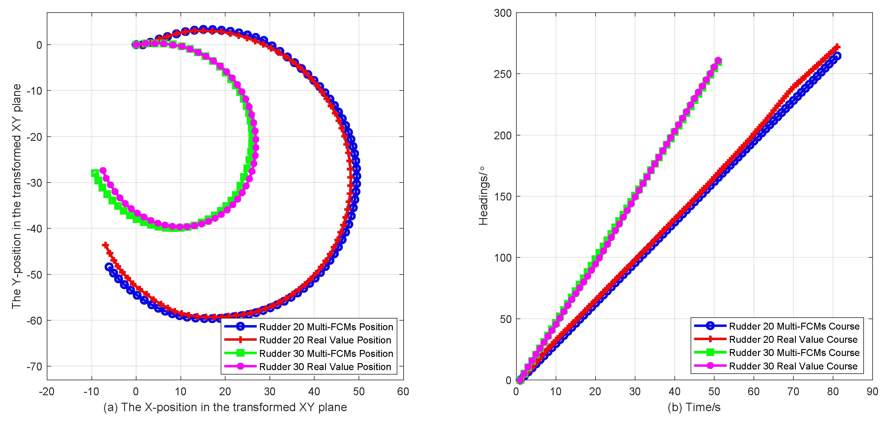
  • The simulation results show that the proposed model is effective and insensitive to speed, as opposed to the classical model. This scheme has potential application value in the field of marine science.
The rest of this paper is organized as follows. In Section 2, we motivate our approach by presenting prior related research. After that, we propose an integrated scheme of data-driven multi-block FCMs to model the steady turning motion of motorboats based on sea trials. The experimental simulations are described in Section 4, while discussions are provided in Section 5. Finally, we provide the conclusions in Section 6.

2. Preliminaries

2.1. Fuzzy Cognitive Maps (FCMs)

An FCM is defined by a four-tuple structure { C , W , A , f } with conceptual nodes and directed edges [43]. The direction of the edges represents the causal relationship, and the weights represent the causal strength.
The symbol C represents the set of conceptual nodes, C = { C 1 , C 2 , , C N } , C i represents the i-th node, and N represents the number of nodes. Nodes are symbols abstracted from the system variables, which are the elements of an FCM.
The expression W : ( C i , C j ) w i j indicates that conceptual node C i has a causal impact on the other node C j with causal strength w i j . The range of w i j is from –1 to 1. If w i j > 0 , the conceptual node C i enhances C j . If w i j < 0 , C i harms C j . If w i j = 0 , C i does not affect C j . W is the adjacency matrix in Equation (1):
W = w 11 w 12 w 1 n w 21 w 22 w 2 n w n 1 w n 2 w n n
The column vector V j = [ w 1 j , w 2 j , , w n j ] T indicates the influence of other conceptual nodes on the j-th node. At this time, the activation value of the j-th node is the dependent variable, and other nodes, except the j-th node, are the independent variables, which constitutes a submodule of the fuzzy cognitive map that can be used to simplify the system.
The symbol A : C i A i represents the activation value of the i-th node. A i ( t ) indicates the activation value of the i-th node after t iterations. A ( 0 ) represents the initial activation values of all nodes. A ( t ) represents the activation values of all nodes after t iterations. f ( x ) represents the activation function. Usually, a hyperbolic tangent or sigmoid function is selected for practical purposes [43,44,45].
The activate value of each node in the FCM updates with iteration. The reasoning mechanism [43] is expressed in Equation (2).
A j ( t + 1 ) = f ( i = 1 , i j N A i ( t ) w i j + A j ( t ) )
The reasoning modes of the high-order fuzzy cognitive map are studied in [44,45]. In practice, an appropriate mode of reasoning is chosen based on our needs.
An FCM is different in the construction of map structure, the settings of hidden nodes, and the semantics between nodes compared with the traditional neural network. The map structure of the FCM can be created by fusing experts’ experiences, system states, and the mechanism models. Furthermore, it has no hidden nodes, and this model is easy to train. The learned weights describe the semantic relationship between these two nodes.

2.2. Mercator Projection

Since the sampling positions occur in the spherical coordinate system and the positions of the proposed model are found at the XY coordinates, we map these data to the XY coordinates through the Mercator projection [46] shown in Figure 1.
Figure 1a is the Earth’s ellipsoid. P N is the North Pole. O and O are the centers of the Earth’s ellipsoid and the parallel of latitude, respectively. O P N is the Earth’s axis. φ defines the latitude, and λ defines the longitude. d φ and d λ are the micro-elements of latitude and longitude, respectively. R denotes the radius of the Equator, which flattens the ellipsoid. r denotes the radius of the parallel of declination. The trapezoidal A B C D on the ellipsoidal surface is a tiny surface formed by the intersection of meridians and parallels of declination. A B is the arc of the meridian, and d A B is the micro-element of A B . P N M and P N N are the two meridians of the Earth’s ellipsoid, respectively. M N is the arc of the Equator, M N = R · d λ , and B C is the arc of the parallel of declination, B C = r · d λ .
Figure 1b illustrates the transformation of the ellipsoidal coordinates to the XY plane using the Mercator projection. The mapped meridians of the ellipsoid are lines with equal spacing and are parallel to each other. x is the distance from the Greenwich meridian to any meridian. y is the distance from the Equator to any declination parallel. d x and d y are the micro-elements of x and y, respectively. The rectangular a b c d is a trapezoidal A B C D on the ellipsoid, transformed into an XY coordinate plane by Mercator projection. The line a b stands for the projection of the arc A B on the meridian. The line b c represents the projection of the arc B C on the declination parallel.
By combining Figure 1a,b, we can obtain the formula for the micro-element of x in Equation (3):
d x = R · d λ
Let b stand for the projection of B on the ellipsoid of the Earth in Figure 1. According to the projection nature of the equiangular, the local scale of any point in any direction is equal in the XY coordinate plane exhibited in Equation (4):
lim A B 0 a b A B = lim B C 0 b c B C
By substituting the symbols in Figure 1b into Equation (4), we can obtain the relationship between the two coordinates in Equation (5):
d y d A B = R · d λ r · d λ = R r
where r = R · cos φ 1 e 2 · sin 2 φ . e is the eccentricity. d A B = R · ( 1 e 2 ) ( 1 e 2 · sin 2 φ ) 3 2 d φ . d y = R · ( 1 e 2 ) 1 e 2 · sin 2 φ · d φ cos φ .
By integrating both sides of Equations (3) and (5), we can obtain the positions of the XY coordinate plane [46] in Equation (6):
x = R · λ y = R · ln [ t a n ( π 4 + φ 2 ) · ( 1 + e · sin φ 1 e · sin φ ) e 2 ]

2.3. Optimal Estimation of Positions at the XY Plane Coordinates

Due to the meridional parts, the samplings are transformed to XY plane coordinates using Mercator projection and are optimized from Equation (7) to Equation (10).
The position measured by the i-th piece of equipment is ( x i , y i ) , i = 1 , 2 , , n . Let the abscissa of the optimal position be x * in Equation (7).
x * = i = 1 n k i · x i
where k i denotes the weight of the abscissa of the i-th GPS sensor.
From the unbiasedness, the relationship between the weights can be found in Equation (8).
i = 1 n k i = 1
From the efficiency, the constraint equation (Equation (9)) is obtained.
arg min k 1 , k 2 , , k n D ( i = 1 n k i · x i ) s . t . i = 1 n k i = 1
Equation (9) can be solved by inverse variance weighting [47], and the weight of each sensor is then calculated in Equation (10).
α = 2 · ( 1 i = 1 n 1 σ i 2 ) k i = α 2 · σ i 2
where α denotes a Lagrange multiplier, and σ i is the i-th systematic variance of GPS sensor. y is obtained in the same way.

3. The Scheme of the Data-Driven Multi-Block FCMs Based on Ship Trials

This section focuses on the multi-block FCMs model based on ship trials. The goal is to demonstrate a practical engineering scheme and verify its potential value. The framework of this scheme is demonstrated in Figure 2. This covers data collection, preprocessing, the construction of the FCMs model, and its application. In what follows, we center this designed framework in our in-depth investigation of the proposed model.

3.1. Sea Trials of Motorboats

Considering the safety, operability, and economy of the sea trials, we measured turning motion using external sensors on the motorboat. Before organizing sea trials, the scheme, instruments, auxiliary kits, methods, layout, contingency measures, and emergency spares had to be prepared.
The plan was to conduct turning tests with a rudder deflection of of 20 ° / 30 ° . The prerequisites were as follows. The water areas are sufficient, the wind does not exceed Beaufort Level 3, the ocean currents are stable, and the ship’s speed reaches its maximum output. In practice, to obtain reliable sampled data, we can increase the number of experiments to reduce the effect of the contingency. The main instruments and other types of equipment are shown in Figure 3.
In Figure 3, part I is a motorboat made of glass-fiber-reinforced plastics that do not measure interference. Part II is a manually recorded rudder angle indicator. Part III is a Garmin sensor used for sampling positions, and its variance is ±7.0 m. Part IV is software that SDI-225R can use to record time series. Part V is an SDI-225R sensor used to sample positions and headings. The sampling frequency is 1 Hz. The variance of the headings is ±0.2 ° , and the variance of the positions is ± 1.0 m. The independent layout of the SDI-225R and Garmin sensors on the motorboat is shown in Figure 4. Figure 4a shows the SDI-225R sites, while Figure 4b displays the locations of all sensors from a top view. We fixed the SDI-F and SDI-S sensors at the centerline and placed the Garmin sensor at the stern. In addition, we prepared other experimental supplies, such as computers, mobile power supplies, belts, scissors, and hand boards.
We had to overcome many adverse factors during the experiments. These factors include the following: (1) The hull was easily damaged. (2) There was a risk of grounding. (3) There was improper listing due to a loss of balance. (4) These apparatuses needed to be fixed individually. (5) A rudder angle indicator needed to be installed and recorded manually. (6) There was an error in manual steering. (7) The sensors had limitations. (8) Other critical factors, such as power persistence, hardware, and software inspection, had to be considered.
The measured data of the motorboat sea trials with a rudder deflection of 20 ° and 30 ° are shown in Table 1. This shows the sensor’s name, data attributes, and data dimensions. The symbol ‘√’ represents the measured data, while the symbol ‘×’ denotes that the measured value is unavailable for this attribute. We employed the Garmin and SDI_225R sensors to measure the positional samplings to enhance the system’s reliability and then applied Equation (10) to optimize these positional samplings.

3.2. Preprocessing for the Samplings of Ship Trials

The samples of ship trials can be affected by disturbances, random noise, and projection transformation. Therefore, it is necessary to preprocess these data. The main task of this section is to visually exhibit the sensor samplings. We performed coordinate transformations twice for the longitude and latitude samplings of Garmin and SDI_225R sensors and used inverse variance weighting to obtain optimized estimations. Finally, we oriented the modeling methodology of the multi-block FCMs.

3.2.1. Samplings from Ship Trials

Constrained by the sensors, we could only extract these samplings after the tests and obtained two data series on the steady turning motion. Subsequently, we imported these collected ‘∗.GPX’ files into the MATLAB [48] in Figure 5.
In Figure 5, the large and small red circles represent the positions sampled by SDI-225R when the command rudder angle is 20 ° and 30 ° , respectively, while the large and small yellow circles represent the positions collected by the Garmin sensor, respectively. The left side of Figure 6 demonstrates the headings sampled by SDI-225R when the rudder angle is 20 ° and 30 ° , respectively. On the right side of Figure 6, the red and blue circles are the longitude and latitude data from the Garmin and SDI-225R sensors, respectively.

3.2.2. Data Fusion for the Multi-Source Position Samplings

In practice, using a variety of sensors to measure the same physical variable is a common strategy to ensure navigation safety. As the sensors installed on the fore and aft centerline collected data independently, we propose a fusion algorithm for multi-source position samplings to obtain optimal estimations.
According to Equation (6), we transformed the sampling data of two sensors from spherical to XY plane coordinates, as shown in Figure 7. The figure shows the mapped position samplings from the ellipsoidal coordinate to the geocentric plane coordinate, obtained by Mercator projection with a rudder deflection of 30 ° , where the red circle and the green cross at the geocentric plane coordinates represent the mapping data corresponding to the Garmin and SDI_225R samplings, respectively.
According to [49], the data transformation form should help to achieve the data mining scheme. Because the data used for training come from historical samplings, the ranges of attributes in the nonlinear ship system vary significantly. The diameter of the ship’s turning circle is approximately 50 m, and the order of magnitude of the geocentric plane coordinates is 10 7 m. Some sampled data, with a rudder deflection of 20 ° according to the Garmin sensor, and their transformed values are shown in Table 2. However, having an excessive number of digits in the geocentric plane coordinates increases the computational burden. The changes in the trajectories of the turning circle will overshadow the differences in coordinates in the geocentric plane, which may lead to the failure of the proposed model. Therefore, it is necessary to translate the sampling coordinates into the water areas, as shown in Equations (11)–(13).
Suppose that X and Y express the position samplings in the geocentric plane coordinates, and their mean values are M X and M Y , respectively. The coordinates ( 0 , 0 ) are then translated to ( M X , M Y ) in Equation (11):
X T = X M X Y T = Y M Y
where X T and Y T denote the positions after translation, and the subscript T represents the new coordinates.
If the positions are derived from the Garmin sensor, then the translated coordinates are described in Equation (12):
X T G = X G M X G Y T G = Y G M Y G
where the superscript G describes the Garmin sensor, and X T G and Y T G represent the positions of the Garmin samplings after translation.
If the positions are from the SDI-225R sensor, then the translated coordinates are described in Equation (13):
X T S = X S M X S Y T S = Y S M Y S
where the superscript S describes the SDI-225R sensor, and X T S and Y T S represent the positions of the SDI-225R samplings after translation.
According to Equation (10), the optimal estimations are expressed in Equation (14):
X T * = K 11 · X T G + k 21 · X T S Y T * = K 12 · Y T G + k 22 · Y T S
where the superscript ∗ describes the optimal value and X T * and Y T * are the optimal positions after translation. k i j is the weight of the i-th sensor in the j-th variable, where i = 1 and i = 2 define the Garmin and SDI-225R sampling data, respectively; j = 1 and j = 2 denote the abscissa and ordinate, respectively.
By substituting Equations (12) and (13) into Equation (14), we can obtain Equation (15):
X T * = ( k 11 · X G + k 21 · X S ) X * ( k 11 · M X G + k 21 · M X S ) M X T * Y T * = ( k 12 · Y G + k 22 · Y S ) Y * ( k 12 · M Y G + k 22 · M Y S ) M Y T *
where X * and Y * are the optimal positions in the geocentric coordinate plane. Equation (15) can then be simplified in Equation (16):
X * = X T * + M X T * Y * = Y T * + M Y T *
We employ two sensors to sample the sea trial of a motorboat as an illustrative example for data preprocessing, as shown in Figure 8. Figure 8a,b demonstrates the position diagram using the SDI-225R, and Garmin sensors and the proposed algorithm after coordinate translation. They are the red circle, the magenta cross, and the green square, respectively. Due to the higher accuracy of the SDI-225R sensor, the optimized estimations are close. Figure 8c,d demonstrate the trajectory errors compared with the optimized values with a rudder deflection of 20 ° and 30 ° . As can be seen from Figure 8, two sensors can ensure measurement reliability. Meanwhile, the optimized results are as close as possible to the sensor samplings, with a higher accuracy.
Figure 9 demonstrates that these optimal positions ( X * , Y * ) in the geocentric coordinate plane were mapped to the spherical coordinate plane by inverse Mercator projection ( φ * , λ * ) . The yellow and red lines are the measured positions of the Garmin and SDI-225R sensors, respectively. The blue line is the optimal estimation derived by combining these two samplings. Because the measurement accuracy of an SDI-225R sensor is higher than that of the Garmin sensor, the red and blue lines almost coincide, which is in line with reality. In summary, the multi-source data fusion scheme can improve the accuracy and reliability of the system.

3.3. A Data-Driven Multi-Block FCMs Model

We usually observe the following four steps when modeling with fuzzy cognitive maps:
  • Step 1: Convert the time series of the sampling into activate values.
  • Step 2: Construct a multi-block FCMs model, then train it with these activations.
  • Step 3: Transform the activations generated by the FCMs model to the actual physical system. An FCM can predict any node’s activation after any iteration given any initial value, which is inversely mapped to the physical space to simulate the actual scenario.
  • Step 4: Apply the trained model to predict or control the system.

3.3.1. Mapping for Activate Values

These samplings were activated by the method in Equation (17) [50]:
A j ( t ) = f ( ( S j ( t ) max ( S j ) + min ( S j ) 2 ) · Λ m a x Λ j ) f ( x ) = 1 1 + e ( η · x )
where A j ( t ) is the activation of the j-th conceptual node at the t step. j is the node number, and j = 1 , 2 , , N . N denotes the number of concept nodes. t denotes the t-th sample, and t = 1 , 2 , , T . T is the number of samples. A is the matrix of activations, and A = A 1 ( 1 ) A 2 ( 1 ) A N ( 1 ) A 1 ( 2 ) A 2 ( 2 ) A N ( 2 ) A 1 ( T ) A 2 ( T ) A N ( T ) . f ( x ) denotes an activation function, and η is a slope parameter. S j is the physical value of the j-th node, where S j = { S j ( 1 ) , S j ( 2 ) , , S j ( T ) } . Λ j is the range of the sampling physical state of the j-th conceptual node, where Λ j = max ( S j ) − min ( S j ) . Λ m a x is the maximum physical state of all nodes, where Λ m a x = max ( Λ 1 , Λ 2 , , Λ N ) .
All physical values are mapped to an open interval between 0 and 1 using Equation (17), which constructs a training dataset learned by a multi-block FCMs model. The advantage is that the trend is consistent between the activations and values of the original system. Meanwhile, considering the monotonicity of the activation function, these activation values can easily be reversely converted to the states of the actual physical system.

3.3.2. The Structure of an FCM for Motorboats

The structure of an FCM can be derived from seamen’s experience. We employed the cognitive structure of steady turning motion for motorboats in Figure 10 and causally represent the FCM in a combination of methods found in [41]. In Figure 10, δ is the angle of the rudder, which was manually recorded. ψ is the heading collected by the SDI-225R sensor. Δ ψ is the difference in the heading. x and y, transformed from the SDI-225R and Garmin sensors in Section 3.2, are the horizontal and vertical coordinates in the XY coordinate plane, respectively. Δ x and Δ y are the diffierences in x and y. In terms of semantics, we used δ and Δ ψ as examples. δ is the cause node, and Δ ψ is the effect node. The connection edge describes the causal influence, which is practically consistent with seafarers’ intuitions.
The interaction between the fuzzy cognitive map and the existing system of motorboats is also demonstrated in Figure 10. The red bar represents normalization data, and the green bar represents mapping to actual physical variables. The red arrow represents the conversion of actual physical variables to normalized data to train the FCM model. The green arrow represents the conversion of the normalized data to actual physical variables performed to predict the system’s state. The time series of the samplings were saved according to the conceptual nodes of the graph model, and the prefix n represents the active value. The system, which determines the interaction between the physical apparatus and the FCM model, comprises a multi-block FCMs model, sensors, and a rudder.
We employ the fuzzy cognitive map constructed by the prior knowledge of seafarers to represent the influences among the ship motion systems, and we then approximated this system using the iterative rules in Equation (2). This simplified network structure is a general expression of a surface vessel.

3.3.3. Modeling of an FCM

As a symbolic reasoning mechanism, Equation (2) performs inverse transformation and data iteration for an FCM, and this equation can be written in matrix form in Equation (18).
f 1 A j ( 2 ) A j ( 3 ) A j ( T ) = A 1 ( 1 ) A 2 ( 1 ) A N ( 1 ) A 1 ( 2 ) A 2 ( 2 ) A N ( 2 ) A 1 ( T 1 ) A 2 ( T 1 ) A N ( T 1 ) · w 1 j w 2 j w N j
When the structure of an FCM is determined, the model parameters can be estimated using activations after mapping.
Since the number of samples is greater than that of conceptual nodes ( T N ), theoretically, Equation (18) is a classical overdetermined linear system of equations without biases, which can be directly solved using the least square method. However, considering that the measured samplings of motorboat motion include external disturbances and are also affected by numerous factors, such as noise, a loss of coordinate transformation, and system nonlinearity, these activations of conceptual nodes near the origin may significantly deviate after mapping. Therefore, it is necessary to use overdetermined linear equations with biases to approximate these activations to reduce this effect. We introduce an offset term w 0 j for each conceptual node to reconstruct the linear equations, as demonstrated in Equation (19):
f 1 A j ( 2 ) A j ( 3 ) A j ( T ) = 1 A 1 ( 1 ) A 2 ( 1 ) A N ( 1 ) 1 A 1 ( 2 ) A 2 ( 2 ) A N ( 2 ) 1 1 A 1 ( T 1 ) A 2 ( T 1 ) A N ( T 1 ) · w 0 j w 1 j w 2 j w N j
Let Y j = f 1 A j ( 2 ) A j ( 3 ) A j ( T ) , Z = 1 A 1 ( 1 ) A 2 ( 1 ) A N ( 1 ) 1 A 1 ( 2 ) A 2 ( 2 ) A N ( 2 ) 1 A 1 ( T 1 ) A 2 ( T 1 ) A N ( T 1 ) , and W j = w 0 j , w 1 j , w 2 j , , w N j T , then Equation (19) is simplified into Equation (20):
Y j = Z W j
where Z and Y j are the independent and dependent variables of the activate values of the historical sampling data, respectively. Therefore, the learning problem of the weights of an FCM is converted into a least square solution of an overdetermined linear system of equations with biases.
We employ the least square method to solve the linear Equation (20) and obtain Equation (21).
W j = ( Z T Z ) 1 Z T Y j
However, the ship motion system is strongly nonlinear, and the prediction error may be significant if only this optimization is used. Furthermore, the optimization is also subject to physical constraints such as the steering gear and the gyrocompass. To solve W j , we construct a new objective function in Equation (22).
a r g m i n W j Z W j Y j 2 , δ L δ δ U , ψ L ψ ψ U s . t . Z τ W τ Y τ 2 ε d         35 ° δ 35 °         0 ° ψ 360 °
Optimization objective of the first term Z W j Y j 2 is to minimize the error between the actual value and the prediction under the double constraints of rudder angle and heading angle to obtain the approximate weight W. The goal of the constraint Z τ W τ Y τ 2 ε d is to alter the approximation accuracy of C τ to adjust the domain range of the rudder angle and heading angle in the first term, and then optimize a reasonable weight. ε d is the designed error, and C τ represents the designed conceptual node. It is contradictory to employ Equation (21) to directly solve Equation (20) because of the constraints of Equation (22). For example, if ε d is too large, the weight after optimization Z W j Y j 2 does not meet the standards of practical applications, and if ε d is too small, there may be no solutions.

3.3.4. Data Split and Training for the Multi-Block FCMs Model

For the constraint Equation (22), the divide-and-conquer strategy is an effective resolution. Under the given ε d , we can train the approximation weight W by reasonably selecting the range of rudder angle and heading angle in the first term. Combined with the actual condition of the ship motion system, it is difficult to approximate with only one fuzzy cognitive map owing to the system’s nonlinearity, and the complete system also needs to be divided into several subblocks for investigation. Therefore, the proposed scheme achieves consistency when solving equations using a data-driven and complex physical system decomposition.
The splitting of samplings is demonstrated in Figure 11. We used two conceptual nodes ( δ and ψ ) to separate the dataset. In our study, the univariate least squares method was utilized to learn the parameters when dividing the dataset based on the node of the rudder angle. When partitioning the dataset with the heading angle node, we used the binary least squares method to learn the parameters. The dataset wis isolated into several subblocks according to ε d . A fuzzy cognitive map approximates each data block. In Figure 11, when the rudder and heading angle are δ τ and ψ τ , we use the first sub-module FCM model to represent the system. Similarly, when the rudder and heading angle are δ ξ and ψ ξ , the n-th sub-module FCM model is selected.
Data splitting is a practical procedure to reduce system complexity during training. Because each sample contains multiple conceptual nodes, we employed a multi-block FCMs model to divide these samplings into several uneven subblocks. Each subblock utilizes an FCM for representation, and several submodels symbolize the entire system. The accuracy of this model will tremendously improve with the encryption of sampling and refinement of the data block. For existing applications, the corresponding submodel in different data blocks can be retrieved according to the current rudder angle and the heading angle. Therefore, these submodels can forecast the system states. The inverse Mercator projection method converts these predictions into a spherical coordinate system. The pseudocode of the fundamental process is shown in Algorithm 1.
Algorithm 1: The pseudocode of a multi-block FCMs model based on ship trials
Jmse 11 00442 i009

4. Experiments

In this section, we investigate the engineering practicability of the scheme. All samplings de frorivedm the marine environment, which contains external interference, measurement noise, and actuator errors. The simulation of the multi-block FCMs model and its parameters are presented in Section 4.1 and Section 4.2, respectively.

4.1. The Steady Turning Simulation with A Rudder Deflection of 20 ° / 30 °

To maintain generality and make comparisons with the proposed model, we translated the initial values to the coordinate origin, and all the time series panned together with the initial values in Figure 12, which displays a diagram of a motorboat turning trajectories and headings with a rudder deflection of 20 ° and 30 ° .
In Figure 12a, we show the measured positions with the red line and the magenta line, respectively. The multi-block FCMs model’s estimations are shown as blue and green lines, respectively. We analyzed these positions with a rudder deflection of 20 ° / 30 ° using three statistical indexes: the root means square errors (RMSEs), the maximum absolute errors (MAEs) and the maximum relative errors (MREs). The i-th position is expressed as P i = x i + y i , where i = 1 , 2 , , T . The i-th position error is then expressed as E P i = P i R e a l P i F C M s . The RMSEs are 1.4506 m and 0.6154 m, the MAEs are 0.8489 m and 0.4721 m, and the MREs are 1.71% and 1.47%, respectively. The results indicate that the proposed model is agreement with the system.
An analogous situation occurs in Figure 12b. The red and magenta lines are the gauged headings, and the blue and green lines are the headings calculated by the proposed model. Similarly, the RMSEs of headings with a rudder deflection of 20 ° / 30 ° are 5 . 0869 ° and 1 . 8384 ° , respectively. The estimations are also consistent with the measurements. These results show the engineering practicability of the proposed model.

4.2. Data Split and Parameters Training

The initial parameters are as follows. The slope parameter η of activations in (17) is 0.01. ε d is [1, 0.1]. The structure of an FCM is exhibited in Figure 10. The reasoning mechanism of an FCM is the sigmoid function, and its parameter is 2. The semi-major and semi-minor axes of the ellipsoid are 6,356,752.3142 m and 6,378,137 m, respectively. The first and second eccentricities are 0.0818191910428 and 0.0820944381519, respectively. The entire system is then isolated into multiple subsystems in Figure 13.
Figure 13 demonstrates the proposed scheme being employed to split the samplings into 17 subblocks. Each data block is approximated by an FCM model. Each number represents the serial number of each block in Figure 13. Table 3 displays the parameters of the motorboat estimated by the multi-block FCMs.
In Table 3, the causal strengths between the headings and the Δ x are 0.47, −1, and 1 in the 1st, 6th, and 17th subblocks, respectively. According to the common sense of navigation, the headings have positive and negative effects on the Δ x , and the adjacency weights reflect this feature. Similarly, the strengths between rudder angles and the heading changes are 0.025, 0.328, and 0.279 in the 1st, 6th, and 17th subblocks, respectively. In practice, the rudder angles only positively affect heading changes, so these adjacency weights are also consistent with reality. These model parameters also indicate that the proposed scheme differs from the traditional neural network method.

5. Discussions

Although the designed model performs well according to the simulation results described in Section 4, it is still necessary to further explore the generalization ability and engineering performance under other rudder angle conditions.
Due to the constraints of the sea trials, the measured data that we collected are limited. To better verify the model proposed in this paper, we compare it with the Nomoto model in the industry and then use the generated data to verify our proposed model’s generalization performance. We then use the multi-block FCMs model to predict the steady motion states of the actual motorboat at other rudder angles and analyze this in combination with existing data resources. Finally, we analyze the engineering performance of the model proposed in this paper.

5.1. Comparison and Validation of the Multi-Block FCMs Model

The principle of our proposed model is entirely different from that of the Nomoto model. In Section 5.1.1, we compare these two methods from the perspective of the impact of speed. Considering the limited data resources of the ship trial, we employ the generated data of the Nomoto model as a supporting dataset to validate the proposed multi-block FCMs model. The experimental verifications under various working conditions are exhibited in Section 5.1.2 and Section 5.1.3, respectively.

5.1.1. Comparison with the Nomoto Model

The Nomoto model [28] is a classical model used to depict the ship’s movement. The differential equations are shown in Equation (23).
ψ ˙ = r r ˙ = 1 T · r + K T · δ x ˙ = U · cos ( ψ ) y ˙ = U · sin ( ψ )
where ψ denotes the headings, r is the yaw rating, and δ represents the rudder angle. x and y denote the positions at XY coordinates. U is the speed over the ground. K and T represent the indices of the Nomoto model.
When we utilize the first-order part of the mathematical model in [3], the hydrodynamic derivatives are calculated using only seven ship parameters in the empirical regression equation in [29]. These derivatives can then approximate the indices of K and T.
The seven parameters of the motorboat in this paper are as follows. The length, beam, and fully loaded draft are 8 m, 2.6 m, and 1.1 m, respectively. The block coefficient is 0.75. The rudder area is 0.285 m 2 . The distance from the center of gravity to the ship’s center is 0.1 m. The speed of the ship is 5.5 knots. The indices of K and T calculated based on the literature [29] are 0.2212 and 1.7219. Therefore, the diameters of the rudder deflection of 20 ° / 30 ° for the steady turning motion solved by Equation (23) are 73 m and 46 m, respectively. The prediction of this model agrees with the actual measurements.
However, the model does not consider the impact of reduction and external disturbances on the speed during turning. When the speed decreases by 20%, the steady turning diameters of the rudder deflection of 20 ° / 30 ° are 58 m and 38 m, respectively. The rudder results of 20 ° are not ideal, which indicates that this model is easily affected by the speed.
Although our model does not measure speed, we observe positional nodes (x, y). The difference operation of the positional nodes (x, y) acquires a change in positional nodes ( Δ x , Δ y ). Based on this, we employ the identity x ( t + 1 ) = x ( t ) + Δ x ( t ) to estimate the x-position. The y-position is estimated in the same way. Here, we employ the change in positional nodes to approximate the speed. Therefore, the speed impact is implicit in our proposed model. We then use the FCM’s structure and the conceptual nodes’ activations to learn the multi-block FCMs model. The results in Figure 12 illustrate the effectiveness of the proposed model. Therefore, this model can avoid a speed impact if the position measurement is accurate.

5.1.2. Validation the Multi-Block FCMs Model Based on the Simulation Data

Here, we employ the generated dataset of the Nomoto model to verify the multi-block FCMs model. Table 4 reports the simulation dataset’s name, attributes, and dimensions. The symbol ‘√’ represents the measured data. The training set consists of the samplings of ship motion with a rudder deflection of 20 ° and 30 ° , while the testing set consists of the predictions of ship motion with a rudder deflection of 22 ° and 28 ° . The validation results are shown in Figure 14.
In Figure 14a, the measured positions with a rudder deflection of 22 ° and 28 ° are represented by red and magenta lines, respectively. Meanwhile, the multi-block FCMs model’s predictions are represented by blue and green lines, respectively. We analyze these positions with a rudder deflection of 22 ° / 28 ° using three statistical indexes: the RMSEs are 0.5413 m and 0.6978 m, the MAEs are 0.3624 m and 0.6126 m, and the MREs are 1.01% and 2.09%, respectively. The results reveal that the proposed model can reasonably simulate the system’s dynamics.
An analogous situation occurs in Figure 14b. The red and magenta lines are the gauged headings, and the blue and green lines are the headings forecasted by the proposed model. Similarly, the RMSEs of headings with a rudder deflection of 22 ° / 28 ° are 2 . 1174 ° and 2 . 0768 ° , respectively. The estimations can also reasonably approximate the measured values.

5.1.3. Validation the Accuracy of the Proposed Model Based on the Adjustment of Samplings

Table 5 illustrates the scheme for validating the multi-block FCMs model when increasing samples. Among them, the training set consists of the samplings at seven different rudder angles, while the testing set also consists of the predictions with 22 ° and 28 ° rudder angles. The validation results are shown in Figure 15.
In Figure 15a, the measured positions with a rudder deflection of 22 ° and 28 ° are represented by red and magenta lines, respectively. The multi-block FCMs model’s predictions are represented by blue and green lines, respectively. Again, we analyze these positions with a rudder deflection of 22 ° / 28 ° using three statistical indexes: the RMSEs are 0.2675 m and 0.3366 m, the MAEs are 0.1976 m and 0.2714 m, and the MREs are 0.54% and 0.97%, respectively. Compared with the results in Figure 14a, the model’s positional prediction accuracy dramatically increased for the statistical indexes of the RMSEs, MAEs, and MREs. These simulation results demonstrate that the proposed model can reflect the system’s dynamics and improve the model’s performance with increased sampled data.
An analogous situation occurs in Figure 15b. The red and magenta lines are the gauged headings, and the blue and green lines are the headings forecasted by the proposed model. Similarly, the RMSEs of headings with a rudder deflection of 22 ° / 28 ° are 0 . 7518 ° and 0 . 6531 ° , respectively. Compared with the results in Figure 14b, the model prediction accuracy for the yaw angle rose sharply for the statistical indicator of the RMSEs. These results mean that, with an increase in training samplings, the proposed model’s accuracy in mimicking the headings has significantly improved. These experimental results validate the effectiveness of the proposed model.
Figure 16 exhibits the data blocks of the trained model acquired by different training sets. Using only the generated data with a rudder deflection of 20 ° and 30 ° , we divided the entire dataset into 11 sub-data blocks. Using the training data with a rudder deflection of 20 ° , 23 ° , 25 ° , 27 ° , 29 ° , and 30 ° to simulate the steady turning motion with a rudder deflection of 22 ° and 28 ° , we divided the dataset into 24 sub-data blocks. From the ranges of the abscissa in Figure 16a,b, it can be observed that sub-data blocks of various intervals can also be generated according to the rudder angle.

5.2. Analysis of the Generalization Ability of the Proposed Model Based on Motorboat Trials

Figure 17 shows the diagram of the turning trajectories of the motorboat with a rudder deflection of 22 ° / 28 ° . In Figure 17a, the red line and the magenta line are the measured trajectories with a rudder deflection of 20 ° / 30 ° , while the blue line and the green line are the predicted values by the proposed model with a rudder deflection of 22 ° / 28 ° . Due to the limitation of the trial conditions, we cannot directly measure the states corresponding to the rudder deflection of 22 ° / 28 ° . However, the trajectories with a rudder deflection of 22 ° / 28 ° are just between a rudder deflection of 20 ° / 30 ° in Figure 17a, which is in line with navigation practice.
In Figure 17b, the red line and the magenta line are the measured headings with a rudder deflection of 20 ° and 30 ° , while the blue line and the green line are the predicted headings with a rudder deflection of 22 ° and 28 ° . Headings are also found between 20 ° and 30 ° . At this time, the slope of the curve indicates that the course change rate increases with the increment of the rudder angle, which indicates that the heading change caused by the change in the unit rudder angle slows down. Therefore, the predicted values are also in line with a common sense of navigation. The predicted values are mapped to the spherical coordinate system using the inverse Mercator projection in Figure 18, which indicates the expected engineering value.

5.3. Practical Performance Analysis of the Proposed Model Only Based on the Garmin Sensor

In engineering, a practical performance analysis will help promote the landing application of the model. In practice, low-precision samplings will adversely affect modeling and lead to method failure. This section mainly focuses on the engineering performance of the model when using low-precision Garmin positional samplings.
We used the learned multi-block FCMs model to simulate the trajectories of a motorboat shown in Figure 19. The red and the magenta lines represent the data sampled only using the Garmin sensor with a rudder deflection of 20 ° and 30 ° .
In Figure 19a, the blue and green lines are the trajectories predicted by the model with a rudder deflection of 20 ° and 30 ° , respectively. In Figure 19b, the blue and green lines are the predicted trajectories of the model, with a rudder deflection of 22 ° and 28 ° , respectively. Figure 20 shows the subblocks diagram of the model that only relies on Garmin sampling with a rudder deflection of 20 ° and 30 ° . We divided the sampled data into 41 blocks, and each subblock was then approximated by an FCM for knowledge representation.
On the premise that other conditions are the same, if Figure 13 is comapared with Figure 20, the number of subblocks split by the sampled data increases from 17 to 41. On the one hand, poor-quality single-source data reduce the accuracy and increase the number of blocks, resulting in a computational burden, which indicates the effectiveness of a multi-source fusion scheme. On the other hand, this model can still approximate the samplings with disturbances, which exhibits its robustness. The simulation results show that the proposed method has a potential engineering application value.

6. Conclusions

The current results of the steady turning motion model of the ship in the shipping industry are insufficient for direct application to motorboats. This paper proposes an integration scheme of data-driven multi-block FCMs for steady turning motions. Sea trials, data sampling, and data processing were performed, and a multi-block FCMs model was established. We can draw the following conclusions from the experimental results:
  • The experimental organization scheme used in this study reduces the risk of sea trials, and the sensors are low-cost and easy to deploy. Investigators need to observe four physical variables during their voyages.
  • The samplings of the sea trials drove the multi-block FCMs model. The validity of the proposed model was verified using a generated dataset of the classical model. The simulation results with a 22 ° /28 ° deflection for motorsboats were consistent with common navigation practices.
  • Compared with models in other studies in the shipping industry, the proposed model reduced speed sensitivity, and thus may have potential application value in nautical science.
However, the data quality and ship time delays were not investigated in-depth in our study. In the future, our team will plan to increase investment in ship trials and collect high-precision samples by updating the system.

Author Contributions

X.G.: Conceptualization, data curation, software, formal analysis, validation, investigation, visualization, writing—original draft. L.W.: writing—review and editing, funding acquisition, resources, project administration. Z.W.: Data curation, software, investigation. X.L.: Conceptualization, methodology, writing—review and editing, resources, supervision, project administration, funding acquisition. All authors have read and agreed to the published version of the manuscript.

Funding

This research is funded by the National Nature Science Foundation of China under grant No.62076049; the Fundamental Research Funds of General Program for the Educational Department of Liaoning Province grant No.LJKZ0043; the 2022 First-class Discipline Seed Fund of Navigation College, DMU, grant No.36330601.

Institutional Review Board Statement

Not applicable.

Informed Consent Statement

Not applicable.

Data Availability Statement

Not applicable.

Acknowledgments

The authors thank the Editor-in-Chief, Associate Editor, and peer reviewers for their valuable comments and suggestions. The authors also would like to thank the faculty in the Water Training Center of Dalian Maritime University for their support of data sampling for the sea trial.

Conflicts of Interest

The authors declare no conflict of interest.

Abbreviations

GPSGlobal positioning system
FCMsFuzzy cognitive maps
USVUnmanned surface vessel
CFDComputational fluid dynamics
MMGManeuvering mathematical modeling group
PRBSPseudo-random binary sequence
CMSPConstrained multi-step prediction
RMSERoot mean square error
MAEMaximum absolute error
MREMaximum relative error

References

  1. IMO. Resolution MSC.137(76); Standards for Ship Manoeuvrability. IMO publishing: London, UK, 2002; pp. 1–6.
  2. IMO. Resolution A.601(15); Recommandation on the Provision and Display of Manoeuvring Information on Board Ships. IMO Publishing: London, UK, 1987; pp. 1–9.
  3. Abkowitz, M.A. Lectures on Ship Hydrodynamics Steering and Manoeuvability; techreport HY-5; Hydro and Aerodynamics Laboratory: Lyngby, Denmark, 1964. [Google Scholar]
  4. Yasukawa, H.; Yoshimura, Y. Introduction of MMG standard method for ship maneuvering predictions. J. Mar. Sci. Technol. 2015, 20, 37–52. [Google Scholar] [CrossRef] [Green Version]
  5. The International Towing Tank Conference. The Manoeuvring Committee Final Report and Recommendations to the 22nd ITTC, Vol. I, Seoul, South Korea and Shanghai, China, 1999; ITTC: Zurich, Switzerland, 1999. [Google Scholar]
  6. The International Towing Tank Conference. The Manoeuvring Committee Final Report and Recommendations to the 29th ITTC, Vol. I, DGA and Ecole Centrale, France, 2021; ITTC: Zurich, Switzerland, 2021. [Google Scholar]
  7. Sano, M.; Yasukawa, H. Maneuverability of a combined two-ship unit engaged in underway transfer. Ocean Eng. 2019, 173, 774–793. [Google Scholar] [CrossRef]
  8. Zhang, C.; Liu, X.; Wan, D.; Wang, J. Experimental and numerical investigations of advancing speed effects on hydrodynamic derivatives in MMG model, part I: Xvv, Yv, Nv. Ocean Eng. 2019, 179, 67–75. [Google Scholar] [CrossRef]
  9. Xu, H.; Guedes Soares, C. Convergence analysis of hydrodynamic coefficients estimation using regularization filter functions on free-running ship model tests with noise. Ocean Eng. 2022, 250, 111012. [Google Scholar] [CrossRef]
  10. Yasukawa, H.; Sakuno, R.; Yoshimura, Y. Practical maneuvering simulation method of ships considering the roll-coupling effect. J. Mar. Sci. Technol. 2019, 24, 1280–1296. [Google Scholar] [CrossRef]
  11. Su, Y.M.; Wang, J.D.; Zhuang, J.Y.; Shen, H.L.; Bi, X.S. Experiments and CFD of a variable-structure boat with retractable twin side-hulls: Seakeeping in waves. Ocean Eng. 2021, 235, 109358. [Google Scholar] [CrossRef]
  12. Nan, X.; Hou, J.M.; Shen, Z.H.; Tong, Y.; Li, G.D.; Wang, X.D.; Kang, Y.D. CFD-DEM coupling with multi-sphere particles and application in predicting dynamic behaviors of drifting boats. Ocean Eng. 2022, 247, 110368. [Google Scholar] [CrossRef]
  13. Park, K.; Kim, D.J.; Kim, S.Y.; Seo, J.; Suh, I.; Rhee, S.H. Effect of waterjet intake plane shape on course-keeping stability of a planing boat. Int. J. Nav. Arch. Ocean 2021, 13, 585–598. [Google Scholar] [CrossRef]
  14. Guo, Y.; Ma, D.L.; Yang, M.Q.; Hu, H.D.; Liu, X. Numerical investigation on the resistance characteristics of a flying boat planing in calm water. Appl. Ocean Res. 2021, 117, 102929. [Google Scholar] [CrossRef]
  15. Sukas, O.F.; Kinaci, O.K.; Bal, S. System-based prediction of maneuvering performance of twin-propeller and twin-rudder ship using a modular mathematical model. Appl. Ocean Res. 2019, 84, 145–162. [Google Scholar] [CrossRef]
  16. Sakamoto, N.; Ohashi, K.; Araki, M.; Kume, K.; Kobayashi, H. Identification of KVLCC2 manoeuvring parameters for a modular-type mathematical model by RaNS method with an overset approach. Ocean Eng. 2019, 188, 106257. [Google Scholar] [CrossRef]
  17. Abkowitz, M. Measurement of hydrodynamic characteristics from ship maneuvering trials by system identification. SNAME Trans. 1981, 88, 283–318. [Google Scholar]
  18. Källström, C.G.; Åström, K.J. Experiences of system identification applied to ship steering. Automatica 1981, 17, 187–198. [Google Scholar] [CrossRef]
  19. Luo, W.L.; Guedes Soares, C.; Zou, Z.J. Parameter identification of ship maneuvering model based on support vector machines and particle swarm optimization. J. Offshore Mech. Arct. Eng. 2016, 138. [Google Scholar] [CrossRef]
  20. Xu, H.T.; Hassani, V.; Guedes Soares, C. Uncertainty analysis of the hydrodynamic coefficients estimation of a nonlinear manoeuvring model based on planar motion mechanism tests. Ocean Eng. 2019, 173, 450–459. [Google Scholar] [CrossRef]
  21. Wang, X.G.; Zou, Z.J.; Hou, X.R.; Xu, F. System identification modelling of ship manoeuvring motion based on support vector regression. J. Hydrodyn. Ser. B 2015, 27, 502–512. [Google Scholar] [CrossRef]
  22. Xu, H.T.; Hinostroza, M.A.; Hassani, V.; Guedes Soares, C. Real-Time parameter estimation of a nonlinear vessel steering model using a support vector machine. J. Offshore Mech. Arct. Eng. 2019, 141. [Google Scholar] [CrossRef] [Green Version]
  23. Bai, W.; Ren, J.; Li, T. Modified genetic optimization-based locally weighted learning identification modeling of ship maneuvering with full scale trial. Future Gener. Comput. Syst. 2019, 93, 1036–1045. [Google Scholar] [CrossRef]
  24. Ouyang, Z.L.; Zou, Z.J. Nonparametric modeling of ship maneuvering motion based on Gaussian process regression optimized by genetic algorithm. Ocean Eng. 2021, 238, 109699. [Google Scholar] [CrossRef]
  25. Ouyang, Z.L.; Chen, G.; Zou, Z.J. Identification modeling of ship maneuvering motion based on local Gaussian process regression. Ocean Eng. 2023, 267, 113251. [Google Scholar] [CrossRef]
  26. Ouyang, Z.L.; Liu, S.Y.; Zou, Z.J. Nonparametric modeling of ship maneuvering motion in waves based on Gaussian process regression. Ocean Eng. 2022, 264, 112100. [Google Scholar] [CrossRef]
  27. Ouyang, Z.L.; Zou, Z.J.; Zou, L. Adaptive hybrid-kernel function based Gaussian process regression for nonparametric modeling of ship maneuvering motion. Ocean Eng. 2023, 268, 113373. [Google Scholar] [CrossRef]
  28. Nomoto, K.; Taguchi, K.; Honda, K.; Hirano, S. On the steering qualities of ships. J. Zosen Kiokai 1956, 1956, 75–82. [Google Scholar] [CrossRef] [PubMed]
  29. Clarke, D.; Gedling, P.; Hine, G. The application of maneuvering criteria in hull design using linear theory. Nav. Archit. 1983, 125, 45–68. [Google Scholar]
  30. Perera, L.P.; Guedes Soares, C. Pre-filtered sliding mode control for nonlinear ship steering associated with disturbances. Ocean Eng. 2012, 51, 49–62. [Google Scholar] [CrossRef]
  31. Perera, L.P.; Guedes Soares, C. Lyapunov and Hurwitz based controls for input–output linearisation applied to nonlinear vessel steering. Ocean Eng. 2013, 66, 58–68. [Google Scholar] [CrossRef]
  32. Moreira, L.; Guedes Soares, C. Dynamic model of manoeuvrability using recursive neural networks. Ocean Eng. 2003, 30, 1669–1697. [Google Scholar] [CrossRef]
  33. Zhang, X.G.; Zou, Z.J. Black-box modeling of ship manoeuvring motion based on feed-forward neural network with Chebyshev orthogonal basis function. J. Mar. Sci. Technol. 2013, 18, 42–49. [Google Scholar] [CrossRef]
  34. Wang, N.; Er, M.J.; Han, M. Large tanker motion model identification using generalized ellipsoidal basis function-based fuzzy neural networks. IEEE T. Cybernetics. 2015, 45, 2732–2743. [Google Scholar] [CrossRef]
  35. Wang, X.D.; Zhao, J.; Liu, S.J.; Geng, T. A constraint multi-step prediction method for identification of a water-jet vessel in 3DOF planar motion. Ocean Eng. 2021, 237, 109534. [Google Scholar] [CrossRef]
  36. Abrougui, H.; Nejim, S.; Hachicha, S.; Zaoui, C.; Dallagi, H. Modeling, parameter identification, guidance and control of an unmanned surface vehicle with experimental results. Ocean Eng. 2021, 241, 110038. [Google Scholar] [CrossRef]
  37. Xiong, Y.; Yu, J.J.; Tu, Y.J.; Pan, L.; Zhu, Q.G.; Mou, J.M. Research on data driven adaptive berthing method and technology. Ocean Eng. 2021, 222, 108620. [Google Scholar] [CrossRef]
  38. Xu, X.L.; Lu, Y.; Liu, X.C.; Zhang, W.D. Intelligent collision avoidance algorithms for USVs via deep reinforcement learning under COLREGs. Ocean Eng. 2020, 217, 107704. [Google Scholar] [CrossRef]
  39. Kosko, R. Fuzzy cognitive maps. Int. J. Man-Mach. Stud. 1986, 24, 65–75. [Google Scholar] [CrossRef]
  40. Felix, G.; Nápoles, G.; Falcon, R.; Froelich, W.; Vanhoof, K.; Bello, R. A review on methods and software for fuzzy cognitive maps. Artif. Intell. Rev. 2019, 52. [Google Scholar] [CrossRef] [Green Version]
  41. Gao, X.R.; Pan, X.J.; Liu, X.D.; Pedrycz, W.; Wang, Z.P. Modeling of the ship steady turning motion based on multiblocks of fuzzy cognitive maps. Appl. Ocean Res. 2021, 110, 102604. [Google Scholar] [CrossRef]
  42. Gao, X.R.; Liu, X.D.; Yan, S.J.; Yu, J.G.; Yang, L.J. Study on the data filling model for the turning motion of the training boat with missing observations. In Proceedings of the 2020 Chinese Automation Congress (CAC), Shanghai, China, 6 November 2020; IEEE: Piscataway NJ, United States, 2020. pp. 7180–7185. [CrossRef]
  43. Stach, W.; Kurgan, L.; Pedrycz, W.; Reformat, M. Genetic learning of fuzzy cognitive maps. Fuzzy Sets Syst. 2005, 153, 371–401. [Google Scholar] [CrossRef]
  44. Yang, S.C.; Liu, J. Time-Series forecasting based on high-order fuzzy cognitive maps and wavelet transform. IEEE Trans. Fuzzy Syst. 2018, 26, 3391–3402. [Google Scholar] [CrossRef]
  45. Lu, W.; Yang, J.H.; Liu, X.D.; Pedrycz, W. The modeling and prediction of time series based on synergy of high-order fuzzy cognitive map and fuzzy c-means clustering. Knowl.-Based Syst. 2014, 70, 242–255. [Google Scholar] [CrossRef]
  46. Kessler, F.C. Projections. In International Encyclopedia of Human Geography; Rob, K., Nigel, T., Eds.; Elsevier: London, UK, 2009; pp. 455–473. [Google Scholar] [CrossRef]
  47. Inverse-Variance Weighting. From HandWiki, Inverse-Variance Weighting. 2021. Available online: https://handwiki.org/wiki/Inverse-variance_weighting (accessed on 13 December 2022).
  48. Help Center. Open Web Map of the Matlab in R2022a, Display Web Map. 2013. Available online: https://ww2.mathworks.cn/help/map/ref/webmap.html?./ (accessed on 13 December 2022).
  49. Han, J.W.; Kamber, M.; Pei, J. Data Mining: Concepts and Techniques, 3rd ed.; Elsevier (Singapore) Pte Ltd: Singapore, 2011; pp. 111–119. [Google Scholar]
  50. Liu, X.D.; Zhang, Y.L. Numerical dynamic modeling and data driven control via least square techniques and Hebbian learning algorithm. Int. J. Numer. Anal. Model 2010, 7, 66–86. [Google Scholar] [CrossRef]
Figure 1. Mercator projection transformation between the ellipsoid coordinate and the XY plane coordinate. (a) Earth ellipsoid coordinate. (b) Projection of the trapezoidal surface at the XY coordinates.
Jmse 11 00442 g001
Figure 2. The framework of data-driven multi-block FCMs model based on motorboat sea trials.
Jmse 11 00442 g002
Figure 3. Main instruments and apparatuses for marine motorboat tests. (I) Motorboat. (II) Rudder recorder. (III) Garmin sensor. (IV) The SDI-225R software. (V) SDI-225R sensor.
Jmse 11 00442 g003
Figure 4. Experimental layout: (a) installation sites; (b) top view of sensors.
Jmse 11 00442 g004
Figure 5. Schematic diagram of the motorboat sampling data in harbor. Red points indicate positions with a rudder deflection of 20 ° .
Jmse 11 00442 g005
Figure 6. Sampling diagram of the sensors during the sea trial of motorboats. (a) Headings with a rudder deflection of 20 ° ; (b) Positions with a rudder deflection of 20 ° ; (c) Headings with a rudder deflection of 30 ° ; (d) Positions with a rudder deflection of 30 ° .
Jmse 11 00442 g006
Figure 7. Sampling transformation diagram from the spherical coordinate to the geocentric coordinate plane with a rudder deflection of 30 ° .
Jmse 11 00442 g007
Figure 8. Graphs of the optimized positions, Garmin positions, and SDI-225R positions after coordinate translation. (a) The trajectories with rudder 20 ° ; (b) the trajectories with rudder 30 ° ; (c) the errors with rudder 20 ° ; (d) The errors with rudder 30 ° .
Jmse 11 00442 g008
Figure 9. Garmin, SDI-225R, and the optimized position are mapped to the spherical coordinate plane by inverse Mercator projection.
Jmse 11 00442 g009
Figure 10. The cognitive structure of the designed FCMs model for motorboats.
Jmse 11 00442 g010
Figure 11. Samplings data split and its system application.
Jmse 11 00442 g011
Figure 12. Simulations of the turning trajectories and headings with a rudder deflection of 20 ° / 30 ° . (a) Trajectories; (b) Headings.
Jmse 11 00442 g012
Figure 13. The boundary of the multi-block FCMs model based on the multi-source sensors with a rudder deflection of 20 ° / 30 ° .
Jmse 11 00442 g013
Figure 14. Simulations of the turning trajectories and headings with a rudder deflection of 22 ° / 28 ° based on dataset of the Nomoto model with two rudders. (a) Trajectories; (b) headings.
Jmse 11 00442 g014
Figure 15. Simulations of the turning trajectories and headings with a rudder deflection of 22 ° / 28 ° based on dataset of the Nomoto model with seven rudders. (a) Trajectories; (b) headings.
Jmse 11 00442 g015
Figure 16. The boundary of the multi-block FCMs model. (a) Training dataset with two rudders; (b) Training dataset with seven rudders.
Jmse 11 00442 g016
Figure 17. Simulations of steady turning motion for a motorboat with a rudder deflection of 22 ° / 28 ° . (a) Trajectories; (b) Headings.
Jmse 11 00442 g017
Figure 18. The diagram of the optimized positions with a rudder deflection of 20 ° and 30 ° and the predictions of the multi-block FCMs model with a rudder deflection of 22 ° and 28 ° .
Jmse 11 00442 g018
Figure 19. Simulations of the trajectories based on the Garmin sensor. (a) Trained values; (b) Predicted values.
Jmse 11 00442 g019
Figure 20. The boundary of the multi-block FCMs model based on the Garmin sensor with a rudder deflection of 20 ° / 30 ° .
Jmse 11 00442 g020
Table 1. The measurements of the motorboat sea trials with a rudder deflection of 20 ° and 30 ° .
Sensor NameData AttributesData Size
TimeLatitudeLongitudeRuddersHeadings
Garmin20 ° ×113 × 4
30 ° ×66 × 4
SDI_225R20 ° ×113 × 4
30 ° ×66 × 4
GPS Compass××20 ° 113 × 2
××30 ° 66 × 2
Table 2. Some sampled data by the Garmin sensor and their transformed values with rudder 20 ° .
No.WGS-84 Coordinate SystemGeocentric XY CoordinateHeadings/°
λ φ X/mY/m
1121.53391638.86596413,529,093.64310564,675,673.8148886073.1
2121.53393238.86597013,529,095.42421744,675,674.6692238376.5
3121.53395038.86597413,529,097.42796824,675,675.2387807080.0
4121.53402638.86597813,529,099.32039964,675,675.8083375983.6
113121.53391638.86595513,529,105.88824954,675,672.5333858981.0
Table 3. Parameters of the multi-block FCMs model of a motorboat.
StructureSemanticsBlocks and Normalized Parameters
{ 1 , [ 0 ° , 3 ° ] } { 6 , [ 49 ° , 138 ° ] } { 17 , [ 312 ° , 358 ° ] }
Jmse 11 00442 i001Intensity of ψ on Δ x 0.47−11
Jmse 11 00442 i002Intensity of δ on Δ x 0.006−0.0550.041
Jmse 11 00442 i003Offset activation Δ x −0.060.359−0.77
Jmse 11 00442 i004Intensity of δ on Δ ψ 0.0250.3280.279
Jmse 11 00442 i005Offset activation Δ ψ −0.01−0.136−0.116
Jmse 11 00442 i006Intensity of ψ on Δ y 1−0.318−0.941
Jmse 11 00442 i007Intensity of δ on Δ y 0.003−0.022−0.051
Jmse 11 00442 i008Offset activation Δ y −0.146−0.0770.843
Table 4. The training dataset generated by the Nomoto model with a rudder deflection of 20 ° /30 ° .
DatasetData AttributesData Size
Timex-Positiony-PositionRuddersHeadings
Training Dataset20 ° 85 × 5
30 ° 58 × 5
Testing Dataset22 ° 80 × 5
28 ° 70 × 5
Table 5. The training dataset generated by the Nomoto model with a rudder deflection of seven rudders.
DatasetData AttributesData Size
Timex-Positiony-PositionRuddersHeadings
Training Dataset20 ° 85 × 5
21 ° 80 × 5
23 ° 75 × 5
25 ° 68 × 5
27 ° 64 × 5
29 ° 59 × 5
30 ° 58 × 5
Testing Dataset22 ° 80 × 5
28 ° 70 × 5
Disclaimer/Publisher’s Note: The statements, opinions and data contained in all publications are solely those of the individual author(s) and contributor(s) and not of MDPI and/or the editor(s). MDPI and/or the editor(s) disclaim responsibility for any injury to people or property resulting from any ideas, methods, instructions or products referred to in the content.

