Investigation of the Spiral Wave Generation and Propagation on a Numerical Circular Wave Tank Model

Abstract

A two-phase incompressible flow model in three-dimensional cylindrical coordinates is applied for oblique wave generation in a numerical circular wave tank. The governing equations are discretized by a finite volume method, and a mass source function is added to reproduce oblique waves through a spiral wave generator positioned at the center of the tank. The volume of fluid method is implemented to track the free surfaces between the air and fluid, and the zonal embedded grid system is adopted to obtain a grid-independent solution in the cylindrical coordinates. A permeable, circumferentially sloping topography (1:7), similar to a natural beach profile, is set up for investigating wave propagation and other characteristics. The simulation and physical experimental results are compared, which show a good agreement in randomly selected water surface elevation profiles and wave heights under the same wave and sloping conditions. The spiral waves are reproduced and propagated in a phenomenon similar to that observed in the physical experiment. The results also show that the wave-breaking positions differ in different wave conditions and suggest a relationship with cross-shore and longshore velocity distribution in terms of incident wave heights and wave-breaking positions in different wave periods on the same sloping topography. Furthermore, this model can be used to investigate the mechanism of longshore current generation and the influences of beach slope on the generated wave propagation in a sloping topography.

1. Introduction

Wave generation and propagation on a sloping beach topography are areas of interest for researchers in offshore and marine engineering, who are continuing to investigate the influence of incident wave breaking on different wave and sloping conditions so that the necessary steps can be taken to prevent the deterioration of coastal areas through erosion and other natural disasters. From the view of coastal engineering, wind-generated waves propagate obliquely along the shore and displace the sands and other materials through the swash and backwash mechanisms on sloping topography. Furthermore, breaking waves generate a mean current that flows parallel to the coast and finally deforms the topography due to cross-shore and longshore sediment transport. To clearly understand the reasons for beach deformation, we need to investigate wave generation and beach deformation in an experimental set-up in which a wave maker can generate oblique waves and propagate on sloping topography. Several studies have been conducted with different experimental facilities using the flat-type wavemaker [1,2,3,4,5,6]. However, generating oblique waves and ensuring the uniformity of longshore current generation without disturbance from the sidewall using the considered wave maker is difficult. To minimize the sidewall effects, Mizuguchi and Horikawa [7] adopted a passive recirculation system for the first time; Visser [8] modified a pump recirculation system to maximize the uniformity of longshore current in regular waves only and found that the generated longshore current should be accurately circulated to maintain longshore uniformity. Shen Liangduo et al. [9] observed that the beach slope strongly influences sediment transport and uniform current generation in the recirculation setup. Although the recirculation system helped with understanding the mechanisms of beach deformation due to longshore current generation and sediment transport in a rectangular wave tank, ensuring the circulation of in-out flow with the recirculation system and reproducing longshore current generation were difficult due to the lack of sufficient longshore length. Additionally, the effects of sidewall reflection were ignored during the experiments with this system.

In addition to the experimental studies, several researchers have developed numerical models for oblique wave generation [10,11,12,13,14,15,16,17]. Multer [10] developed an exact nonlinear model for wave generation; Nakayama [11] and Lee et al. [12] implemented a boundary element method and a finite element method for solving wave-making problems. Lee et al. [13] proposed a flap-type wave maker for wave generation in the computational domain. However, the effective area was not substantially enlarged using the abovementioned model. To solve this problem, William and Crull [14] and Shih et al. [15] proposed a 3D wave tank model for oblique and multi-directional wave generation. Park et al. [16,17] used an incompressible Navier-Stokes solver to predict non-linear 3D wave fields. Although enlarging the effective area in a rectangular wave basin was possible, the performance was still affected by the side boundary and incident wave direction. Li and Shibayama [18] proposed a numerical model in which a pump was adopted to reduce the effect of the side boundary on the longshore current generation; however, wave reflection still occurred in the effective zones of the wave generator and side boundary. To solve these problems, Larsen and Dancy [19] implemented internal wave generation in a Boussinesq equation model, where the waves were generated inside the computational domain; they adopted the concept of sponge layers proposed by Israeli and Orszag [20] for outgoing wave absorption as open boundaries. Lin and Liu [21] extended the model to the Navier-Stokes equations model, including the source term in the mass conservation equation. Choi and Yoon [22] added the source term to the momentum equation to unidirectionally generate regular or irregular waves. Furthermore, Brorsen and Larsen [23] proposed a non-reflective wave generator. Ohyama and Nadaoka [24] incorporated a wave generator in a BEM-based numerical wave tank model; however, including the wave breaking and post-breaking wave deformation processes in the BEM was not possible. In addition, Tanaka et al. [25] developed a non-reflection circular wave basin model for oblique wave generation; Naito [26] arranged a wave absorption filter at the circular wave tank wall and explained the performance of a circular wave basin. Ren et al. [27] considered a non-reflective wave generator positioned at the sidewall boundary for oblique and multidirectional wave generation [28] and a wave absorption filter for outgoing wave dissipation in a circular wave tank model.

The surface tracking between the air and water interface is also another issue in the numerical modeling. To achieve this, several free-surface tracking methods such as the volume of fluid [29], marker and cell [30] and level set [31] methods, have been considered in numerical studies. Austin and Schulter [32] applied the SOLA-VOF (Nichols et al. [33]) method for wave prediction in a porous armour layer, and Iwata et al. [34] modified it to investigate wave breaking with a submerged structure. Within the above-mentioned developed numerical wave tank model, a wave generator was set up on the side boundary of the wave tank. As a result, observing the influence of the returning flow distribution and longshore current reproduction in the wave tank model was difficult, as was maintaining the uniformity of longshore current during the computation.

To overcome the aforementioned issues of spiral wave generation, uniformity of longshore current distribution, and side wall effects during their experiment, Dean and Dalrymple [35] developed a circular wave-making tank in which spiral waves were obliquely generated with a fixed angle by a cylindrical wave maker. Mei [36] modified this wave maker (Dean and Dalrymple [35]) to increase the incident wave angle and found that the wave-breaking followed the same pattern as plane waves. Trowbridge et al. [37] used an eccentrically mounted rotating cylindrical wave maker to generate spiral waves and observed that the wave amplitude and eccentricity were smaller than the wave maker radius, wavelength, and water depth. However, the influence of the gap between the basin floor and wave maker was unclear, so this was considered by Williams and McDougal [38], who found the wave amplitude decreased with the increase in the gap. Suh and Dalrymple [39] found that the incident wave angle and wave amplitude decayed in a milder sloping beach, which is the major disadvantage of a circular wave basin. However, using the above off-centered rotating circular cylinder as a wave generator, the amplitude and incidence wave angle were fixed by the cylinder diameter, and the generated wave amplitudes and the incident wave angles gradually decreased if the waves passed a far radial distance from the wave generator. The cylinder diameter needed to be enlarged to increase the incident wave height to the desired value and keep the eccentricity smaller; more power was also required for wave generator movement during the experiment. A non-rotating spiral wave maker can be applied to solve the above-mentioned issues and investigate the effects of wave characteristics on the desired wave conditions. To achieve this, Islam et al. [40] conducted experiments using a nonrotating wave generator and found that the waves were spirally generated without the influence of the sidewall boundary and the wave amplitude depended on the rotation speed of the wave maker, not on the size of the wave maker radius, which was claimed in the previous studies.

Considering the study of Islam et al. [40] and assumptions in previous studies, we modified and considered the two-phase incompressible flow model of Ren et al. [27] in 3D cylindrical coordinates in this study. We discretized the governing equations by a finite volume method, and we added a mass source term to the continuity equation as a non-reflective wave generator for oblique wave generation along the circumference of the circular wave tank. The free surface between the air and fluid was captured by the volume of fluid method (VOF), and a high-resolution scheme based on the concept of donor-acceptor as in the VOF was applied to compute the volume fraction of the surface flow simulation in this model. To obtain a grid-independent solution in the computational domain, we applied a zonal embedded grid system in the cylindrical coordinates. We implemented a permeable circumferential sloping beach (1:7) along the circumference of the wave basin, similar to Islam et al. [40]. We compared the wave characteristics and performance differences between the simulation and experimental (Islam et al. [40]) results under the same wave and sloping conditions. In addition, we observed the wave generation and propagation in the present wave tank model; finally, we determined the relationships between the wave-breaking positions and cross-shore and longshore velocity distributions in different wave conditions in the sloping wave tank model.

The remainder of this paper is organized as follows: Section 2 describes the governing equations, and a brief discussion about the methodology, including discretization and grid generation, is provided in Section 3. The computation parameters and conditions are given in Section 4; the spiral wave generation and performance of the adopted wave maker under different wave conditions are described in Section 5, as are the computational results used to validate the wave tank model through comparison with the hydraulic experiment results (Islam et al. [40]). In addition, the findings regarding the incident wave breaking and cross-shore and longshore velocity distributions on the sloping topography are discussed in this section. Finally, the recommendations for further research using the proposed wave tank model are explained in the Conclusions.

2. Governing Equations

To simulate the wave generation and propagation in a circular wave tank, the governing equations are considered in a 3D cylindrical coordinate system where the one-fluid assumption is applied to consider the movement of airflow and water in a two-phase incompressible fluid model. The continuity equation is re-written with a mass source term added to the right side of the equation for wave generation and the modified Navier-Stokes equations are re-written with the source terms in the cylindrical computational domain. To consider a sandy beach consisting of permeable material, the basic equations of the incompressible viscous fluid including the gap of the sand layer proposed by Mizutani et al. [41] and Nakamura and Mizutani [42] are considered in this model. The transformed continuity equation is written as:

$$\frac{1}{r}\frac{\partial \left(r{m}_{r}u\right)}{\partial r}+\frac{1}{r}\frac{\partial m_{\theta }v}{\partial \theta }+\frac{\partial m_{z}w}{\partial z}=Q\left(r_s,{\theta }_s,z,t\right)$$

(1)

where $u,v,w$ and $m_r,m_{\theta },m_z$ are the velocities and porosities in the $r,\theta ,z$ directions, respectively; $Q\left(r_s,{\theta }_s,z,t\right)$ is the mass source term which is only non-zero at the active wave source zone. To incorporate a nonreflecting internal wave maker in the numerical study, Kawasaki [43] and Lin and Liu [21] considered a mass source term acting as an internal wave generator in a two-dimensional numerical model. According to certain wave theory, the wave potential $\varphi \left(r,\theta ,z,t\right)$ can be used to derive the wave source term and the mass source term can be calculated using the formula given by Brorsen and Larsen [23] as

$$Q\left(r_s,{\theta }_s,z,t\right)=2\underset{-h}{\overset{\eta }{{\displaystyle \int }}}{{\displaystyle \int }}_{{\theta }_i}^{{\theta }_i+2\pi }u\left(r,\theta ,z,t\right)dzd\theta /V_s=2\underset{-h}{\overset{\eta }{{\displaystyle \int }}}{{\displaystyle \int }}_{{\theta }_i}^{{\theta }_i+2\pi }\frac{\partial \varphi \left(r,\theta ,z,t\right)}{\partial r}dzd\theta /V_s$$

(2)

where $V_s=\Delta r\underset{-h}{\overset{\eta }{{\displaystyle \int }}}{{\displaystyle \int }}_{{\theta }_i}^{{\theta }_i+2\pi }dzd\theta$ is the total volume of the wave source zone; $\eta$ is the water surface elevation; h is the water depth; ${\theta }_i$ is the incident wave direction; $\Delta r$ is the distance between two cells in the radial direction and coefficient 2 is used for defining the wave generation on both sides of the internal wave source zone. By considering porous media and mass source terms in the present model, the modified momentum equations in cylindrical coordinates are written as

$$\begin{gathered} \frac{\partial \left[\left\{m_r+C_A\left(1-m_r\right)\right\}u\right]}{\partial t}+u\frac{\partial m_{r}u}{\partial r}+\frac{v}{r}\frac{\partial m_{r}u}{\partial \theta }+w\frac{\partial m_{r}u}{\partial z}-m_r\frac{v^2}{r}=-\frac{m_r}{\rho }\frac{\partial p}{\partial r}+ \\ \nu \left\{\frac{{\partial }^2\left(m_{r}u\right)}{\partial r^2}+\frac{1}{r}\frac{\partial \left(m_{r}u\right)}{\partial r}+\frac{1}{r^2}\frac{{\partial }^2\left(m_{r}u\right)}{\partial {\theta }^2}+\frac{{\partial }^2\left(m_{r}u\right)}{\partial z^2}-m_r\frac{u}{r^2}-\frac{2}{r^2}\frac{\partial \left(m_{\theta }v\right)}{\partial \theta }\right\}+\frac{m_r}{\rho }{R}_r+Q_r \end{gathered}$$

(3a)

$$\begin{gathered} \frac{\partial \left[\left\{m_{\theta }+C_A\left(1-m_{\theta }\right)\right\}v\right]}{\partial t}+u\frac{\partial m_{\theta }v}{\partial r}+\frac{v}{r}\frac{\partial m_{\theta }v}{\partial \theta }+w\frac{\partial m_{\theta }v}{\partial z}+m_{\theta }\frac{uv}{r}=-\frac{m_{\theta }}{r\rho }\frac{\partial p}{\partial \theta }+ \\ \nu \left\{\frac{{\partial }^2\left(m_{\theta }v\right)}{\partial r^2}+\frac{1}{r}\frac{\partial \left(m_{\theta }v\right)}{\partial r}+\frac{1}{r^2}\frac{{\partial }^2\left(m_{\theta }v\right)}{\partial {\theta }^2}+\frac{{\partial }^2\left(m_{\theta }v\right)}{\partial z^2}-m_{\theta }\frac{v}{r^2}+\frac{2}{r^2}\frac{\partial \left(m_{r}u\right)}{\partial \theta }\right\}+\frac{m_{\theta }}{\rho }{R}_{\theta }+Q_{\theta } \end{gathered}$$

(3b)

$$\begin{gathered} \frac{\partial \left[\left\{m_z+C_A\left(1-m_z\right)\right\}w\right]}{\partial t}+u\frac{\partial m_{z}w}{\partial r}+\frac{v}{r}\frac{\partial m_{z}w}{\partial \theta }+w\frac{\partial m_{z}w}{\partial z}=-\frac{m_z}{\rho }\frac{\partial p}{\partial z}+ \\ \nu \left\{\frac{{\partial }^2\left(m_{z}w\right)}{\partial r^2}+\frac{1}{r}\frac{\partial \left(m_{z}w\right)}{\partial r}+\frac{1}{r^2}\frac{{\partial }^2\left(m_{z}w\right)}{\partial {\theta }^2}+\frac{{\partial }^2\left(m_{z}w\right)}{\partial z^2}\right\}-m_{z}g+\frac{m_z}{\rho }{R}_z+Q_z \end{gathered}$$

(3c)

where $C_A$ is the added mass coefficient for sand (additional mass coefficient of the permeable material); $\rho$ is the density; $\mu$ is the viscosity; $\nu =\mu /\rho$ is the kinematic viscosity; $R_r, R_{\theta }, R_z$ are the linear and non-linear resistance vectors due to a permeable material and $Q_r,Q_{\theta },Q_z$ are the wave-making source vectors in the $r,\theta ,z$ directions, respectively; $P$ is the pressure; $t$ is the time; $g$ is the gravitational acceleration.

The resistance vectors on the right side of (3a)–(3c) are expressed as:

$$R_i=-\frac{12C_{D2}\mu \left(1-m_i\right)}{m_i{d}_{50}^2}\Phi -\frac{C_{D1}\rho \left(1-m_i\right)}{2m_i{d}_{50}}\Phi \sqrt{u^2+r^2{v}^2+w^2}; i=r,\theta ,z$$

(4)

The above resistance vectors can be subdivided and written as

$$R_1=-\frac{C_{D1}\rho \left(1-m_i\right)}{2m_i{d}_{50}}\Phi \sqrt{u^2+r^2{v}^2+w^2} \mathrm{and} R_2=-\frac{12C_{D2}\mu \left(1-m_i\right)}{m_i{d}_{50}^2}\Phi$$

(5)

where $C_{D1}$ and $C_{D2}$ are the non-linear and linear resistance coefficients, respectively; $d_{50}$ is the median particle size; and $m_i$ is the porosity in the $r,\theta ,z$ directions.

The wave-making source vectors are expressed as:

$$Q_i=\Phi Q\left(r_s,{\theta }_s,z,t\right)-\frac{2}{3}\frac{1}{\rho }\frac{\partial }{\partial x_i}\left[m\mu \left\{\frac{1}{r}\frac{\partial \left(ru\right)}{\partial r}+\frac{1}{r}\frac{\partial v}{\partial \theta }+\frac{\partial w}{\partial z}\right\}\right] ; i=r,\theta ,z$$

(6)

where $Q\left(r_s,{\theta }_s,z,t\right)$ is the wave source function; $m$ is the porosity; and $\Phi$ represents $u, v, w$ depending on the $r,\theta ,z$ directions, respectively.

The VOF method (Hirt and Nichols [29]) is implemented to track the free surface with a scalar indicator function $F$ ($0\le F\le 1$), defined as the volume fraction; marking the fluid occupied in a control volume of the computational domain, the density and viscosity terms of the momentum equations are written as

$$\begin{gathered} \rho =F{\rho }_w+\left(1-F\right){\rho }_a \\ \mu =F{\mu }_w+\left(1-F\right){\mu }_a \end{gathered}$$

(7)

where ${\rho }_a, {\mu }_a$ and ${\rho }_w,{\mu }_w$ are the density and viscosity of air and water respectively. The free surface transport convection equation of the volume of fraction including the mass source in cylindrical coordinates is written as

$$\frac{\partial F}{\partial t}+\frac{1}{r}\frac{\partial ruF}{\partial r}+\frac{v}{r}\frac{\partial Fv}{\partial \theta }+\frac{\partial wF}{\partial z}=Q\left(r_s,{\theta }_s,z,t\right)F$$

(8)

3. Methodology of the Numerical Model

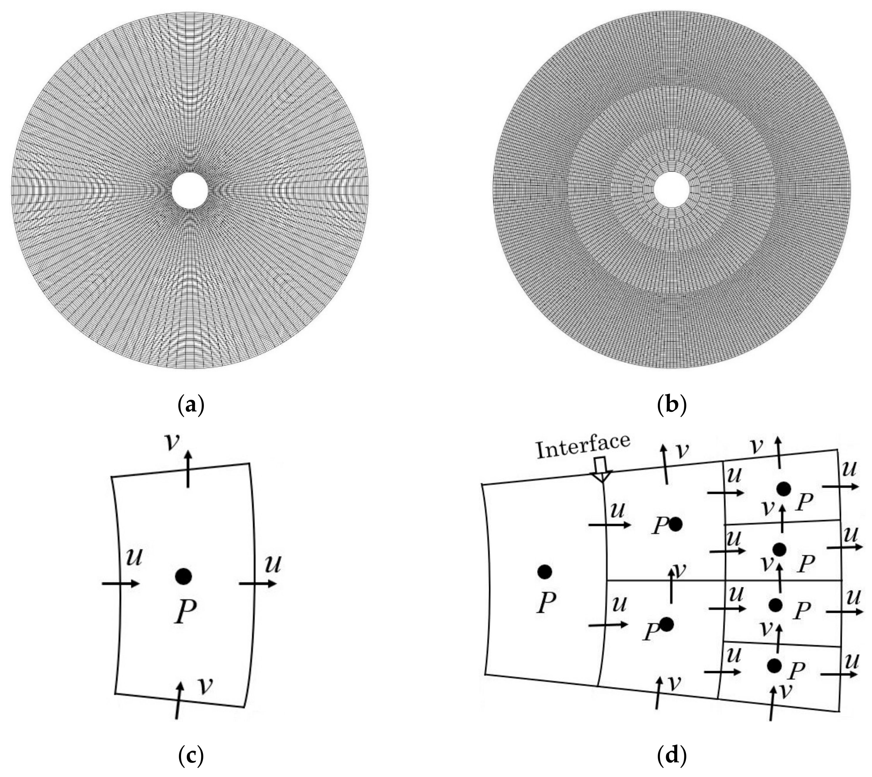
3.1. Grid Generation

In the cylindrical coordinate system, the grid spacing in the azimuth direction differs and is proportional to the radial distance from the origin. The spacing of the grids positioned nearest to the center is smaller than that of the grids positioned at the outer boundary in the application of a regular orthogonal grid system (Figure 1a). So, the control cells become much coarser far from the origin compared with the cells near the origin in the computational domain of a comparatively larger circular wave tank model. A small time step is required for numerical stability during the computation. To obtain the grid-spacing-independent computational domain and take a much larger time step, Kravchenko et al. [44] proposed a zonal embedded grid technique for the first time, and Suh and Yeo [45] implemented the technique for the computation of two-dimensional Navier–Stokes equations in polar coordinates. In this grid system, the entire computational domain is first subdivided into several zones with concentric circles, and the grids in each zone are computed in the same way as the regular grids. The number of grids in each zone differs from one zone to another along the radial and azimuth directions, but the spacing of the radial distances in each zone are the same. The azimuth grid spacings can be independently adjusted as shown in Figure 1b, and the time step can be made substantially larger than that with the regular orthogonal grid system in this grid technique. The above-mentioned zonal embedded grid techniques are adopted in the circular computational domain of this wave tank model.

3.2. Discretization of the Governing Equations

In this study, we discretized the control equations by the finite volume method, and we reformulated the momentum equations in cylindrical coordinates into a general form before discretization according to Xue et al. [46] and He et al. [47] as

$$\begin{gathered} \frac{\partial \left[\left(m+C_A\left(1-m\right)\right)U\right]}{\partial t}+\left(u\frac{\partial \left(mU\right)}{\partial r}+\frac{v}{r}\frac{\partial \left(mU\right)}{\partial \theta }+w\frac{\partial \left(mU\right)}{\partial z}\right)\hspace{1em}\hspace{1em} \\ \hspace{1em}\hspace{1em}\hspace{1em}\hspace{1em}=\left(\frac{1}{r}\frac{\partial }{\partial r} \left(\upsilon r\frac{\partial \left(mU\right)}{\partial r}\right)+\frac{1}{r}\frac{\partial }{\partial \theta } \left(\frac{\upsilon }{r}\frac{\partial \left(mU\right)}{\partial \theta }\right)+\frac{\partial }{\partial z} \left(\upsilon \frac{\partial \left(mU\right)}{\partial z}\right)\right)+S_U \end{gathered}$$

(9)

$$\begin{gathered} u:S_U=-\frac{1}{\rho }{m}_r\frac{\partial p}{\partial r}-\nu \left(\frac{2}{r^2}\frac{\partial \left(m_{\theta }v\right)}{\partial \theta }+m_r\frac{u}{r^2}\right)+m_r\frac{v^2}{r}+\frac{m_r}{\rho }{R}_r+Q_r \\ v:S_U=-\frac{1}{\rho }\frac{m_r}{r}\frac{\partial p}{\partial r}+\frac{\nu }{r}\left(\frac{2}{r}\frac{\partial \left(m_{r}u\right)}{\partial \theta }-m_{\theta }\frac{v}{r}\right)-m_{\theta }\frac{uv}{r}+\frac{m_{\theta }}{\rho }{R}_{\theta }+Q_{\theta } \\ w:S_U=-\frac{1}{\rho }{m}_z\frac{\partial p}{\partial z}-m_{z}g+\frac{m_z}{\rho }{R}_z+Q_z \end{gathered}$$

where $U=\left(u,v,w\right)$ is the velocity; $S_U$ is the source term; $\rho$ is the density; and $\mu$ is the viscosity.

To arrange the grids for the normal control cell and the interface of the coarse and fine blocks’ control cell, the staggered grid arrangement introduced by Harlow and Welch [30] is considered in this model, in which the velocities are stored at the cell faces and the pressure, density, and viscosity are stored at the center of the control volumes, as shown in Figure 1c,d. With a staggered grid arrangement, the projection method (Chorin [48]) is used to iteratively calculate the velocities and pressure for the discretization of the continuity and N-S equations. An intermediate velocity $U^{\ast }$ is first calculated in the projection method and then projected into a divergence-free field by Equations (10) and (11). The second-order Adams-Bashforth (AB) scheme is applied to calculate the approximate velocity and pressure in the convection and diffusion terms in this numerical model.

$$\begin{array}{c} \frac{\left(m^n+C_A\left(1-m^n\right)\right)U^{\ast }-\left(m^n+C_A\left(1-m^n\right)\right)U^n}{\Delta t}\hfill \\ =-{\left(u\frac{\partial \left(mU\right)}{\partial r}+\frac{v}{r}\frac{\partial \left(mU\right)}{\partial \theta }+w\frac{\partial \left(mU\right)}{\partial z}\right)}^n\hfill \\ +{\left(\frac{1}{r}\frac{\partial }{\partial r} \left(\upsilon r\frac{\partial \left(mU\right)}{\partial r}\right)+\frac{1}{r}\frac{\partial }{\partial \theta } \left(\frac{\upsilon }{r}\frac{\partial \left(mU\right)}{\partial \theta }\right)+\frac{\partial }{\partial z} \left(\upsilon \frac{\partial \left(mU\right)}{\partial z}\right)\right)}^n+S_U^n\hfill \end{array}$$

(10)

$$\begin{gathered} U_i{}^{n+1}=\frac{\left(m^n+C_A\left(1-m^n\right)\right)}{\left(m^{n+1}+C_A\left(1-m^{n+1}\right)\right)}{U}^{\ast }-\frac{m^n}{{\rho }^n}\frac{\Delta t}{\left(m^{n+1}+C_A\left(1-m^{n+1}\right)\right)}\nabla \left(P^{n+1}-P^n\right) \\ \stackrel{P^{\prime }=P^{n+1}-P^n}{\Rightarrow } U^{n+1}=U^{\ast }-\frac{m^n}{{\rho }^n}\frac{\Delta t}{\left(m^{n+1}+C_A\left(1-m^{n+1}\right)\right)}\nabla P^{\prime } \end{gathered}$$

(11)

Here, $n$ and $n+1$ denote the previous and new time steps of computation, respectively. The porosity does not change over time; that is, $m^n=m^n+1$. Multiplying both sides of Equation (11) by $m^{n+1}$ and taking the divergence on both sides, the pressure Poisson equation becomes

$$\nabla .U^{\ast }=\frac{m^n\Delta t}{\left(m^{n+1}+C_A\left(1-m^{n+1}\right)\right)}\nabla .\frac{1}{{\rho }^n}{\nabla }_i\left(p^{\prime }\right)$$

(12)

In the discretization procedure using the finite volume method, the entire computational domain is first divided into a set of control volumes of regular or irregular grids in size and shape, then the equations are integrated over the control volumes to transform the control equations from continuous form to discretized form. In this case, the approximated velocity is calculated by the discretized equation derived from the integrations of the Equation (10) over the control volumes. The Equation (10) becomes

$$\begin{gathered} {{\displaystyle \int }}_{\Delta v}^{}\frac{\left(m^n+C_A\left(1-m^n\right)\right)U^{\ast }-\left(m^n+C_A\left(1-m^n\right)\right)U^n}{\Delta t}dv+{{\displaystyle \int }}_{\Delta v}^{}{\left(u\frac{\partial \left(mU\right)}{\partial r}+\frac{v}{r}\frac{\partial \left(mU\right)}{\partial \theta }+w\frac{\partial \left(mU\right)}{\partial z}\right)}^{n}dv= \\ {{\displaystyle \int }}_{\Delta v}^{}{\left(\frac{1}{r}\frac{\partial }{\partial r} \left(\upsilon r\frac{\partial \left(mU\right)}{\partial r}\right)+\frac{1}{r}\frac{\partial }{\partial \theta } \left(\frac{\upsilon }{r}\frac{\partial \left(mU\right)}{\partial \theta }\right)+\frac{\partial }{\partial z} \left(\upsilon \frac{\partial \left(mU\right)}{\partial z}\right)\right)}^n+{{\displaystyle \int }}_{\Delta v}^{}{S}_U^{n}dv \end{gathered}$$

(13)

where $\Delta v$ denotes the control volume. To transform the volume integration over the control volume into the surface integration over the cell faces, Gauss divergence theory is implemented in this model and Equation (13) can be written as:

$$\begin{array}{c}\frac{\left(m^n+C_A\left(1-m^n\right)\right)U^{\ast }-\left(m^n+C_A\left(1-m^n\right)\right)U^n}{\Delta t}\hfill \\ =\frac{1}{\Delta V}{\displaystyle \sum }mflux{U}_f^n\Delta s+\frac{1}{\Delta V}{\displaystyle \sum }m\upsilon \nabla U_f^n\Delta s+\frac{1}{\Delta V}{S}_U^n\Delta V\hfill \end{array}$$

(14)

where $U_f$ is the velocity of the control volume at the cell faces; $\Delta s$ is the surface area of the cell faces; and $flux$ is the mass flux at the cell faces.

To avoid unphysical oscillatory behaviors in regions of flow, the high-resolution scheme named the sharp and monotonic algorithm for realistic transport (SMART) scheme proposed by Gaskell and Lau [49], is used in the numerical computation of $U_f$. The central difference scheme is implemented to compute the mass flux and the gradient velocity $\nabla U_f$ in this model. Considering the above-discussed calculation procedures, we obtain the discretized form of the approximated velocity and then project the approximated velocity into a divergence field with Equation (11). So, the corrective equation can be discretized as

$$\frac{1}{\Delta t}\sum m{U}_f^{\ast }\Delta s=\frac{1}{{\rho }^n}\sum \frac{m}{\left(m+C_A\left(1-m\right)\right)}\nabla P_f^{\text{'}}\Delta s$$

(15)

where $\nabla P_f^{\text{'}}$ is the gradient of corrective pressure at the cell face. The gradients of the pressure and corrective pressure are usually computed using the central difference scheme.

As zonal embedded grids are considered in the numerical model, the discretization features in the control volumes at the interface of coarse and fine blocks are different from the regular ones in the computational domain. To calculate the pressure gradient at the interfacial neighboring cells, we adopted the interpolation scheme introduced by Popinet [50] in this present study as follows

$$\begin{gathered} P_1=\frac{15}{16}{P}_P-\frac{3}{32}{P}_S+\frac{5}{32}{P}_N \\ {P}_2=\frac{15}{16}{P}_P-\frac{3}{32}{P}_N+\frac{5}{32}{P}_S \end{gathered}$$

(16)

where $P_P$, $P_N$, and $P_S$ represent the pressures at the neighbouring cells of the interfaces of two blocks. The Algebraic- Multi-grid (AMG) method developed by Notay [51] is used to solve the discretized pressure Equation (15) and obtain the corrective pressure term and finally the corrective velocity.

To ensure computational stability, we discretize the linear resistance term ($R_2$) by the first-order Euler implicit scheme and the non-linear resistance term ($R_1$) by the first-order Euler explicit scheme of the resistance vectors (Equation (5)), because the value of the median grain diameter ($d_{50})$ is small. As a result, the linear resistance term ($R_2$) may cause instability in the computation. We used the high-resolution Compressive Interface Capturing Scheme for Arbitrary meshes (CICSAM) method proposed by Ubbink and Issa [52] for unstructured grids system to discretize the VOF convection equation, which we extended to the zonal embedded grid system in this study. In the original CICSAM method, the implicit Crank-Nicholson method is used to approximate the volume fractions, and a corrective iterative procedure is applied to modify the unphysical volume fraction. To simplify the computation, the Jacobi-type dual-time-stepping formulation introduced by Heyns et al. [53] is implemented to approach the implicit procedure as

$$\begin{gathered} \frac{F^{\tau +1}-F^{\tau }}{\Delta \tau }+\frac{F^{\tau }-F^n}{\Delta \tau }=Q\left(r_s,{\theta }_s,z,t\right)F^n-\frac{1}{2}(\frac{1}{r}\frac{\partial ru{F}^{\tau }}{\partial r}+\frac{v}{r}\frac{\partial v{F}^{\tau }}{\partial \theta }+\frac{\partial w{F}^{\tau }}{\partial z}+\frac{1}{r}\frac{\partial ru{F}^n}{\partial r}+ \\ \frac{v}{r}\frac{\partial v{F}^n}{\partial \theta }+\frac{\partial w{F}^n}{\partial z}) \end{gathered}$$

(17)

In the above-mentioned procedure, the implicit solution of the VOF convection equation can be approached by the explicit method as it converges in pseudo time $\tau$. The discretized form of Equation (17) in the finite volume method is written as

$$\begin{gathered} \frac{F^{\tau +1}-F^{\tau }}{\Delta \tau }+\frac{F^{\tau }-F^n}{\Delta t}=Q\left(r_s,{\theta }_s,z,t\right)F^n\hspace{1em}\hspace{1em}\hspace{1em} \\ \hspace{1em}\hspace{1em}\hspace{1em}\hspace{1em}\hspace{1em}-\frac{1}{2}\left(\frac{1}{\Delta v}\sum flux{F}_f{}^{\tau }\Delta S+\frac{1}{\Delta v}\sum flux{F}_f{}^n\Delta S\right) \end{gathered}$$

(18)

where $F_f^{\tau }$ and $F_f^n$ are the volume fractions at the faces of the control volumes computed with the CICSAM scheme, and $\Delta \tau$ is the pseudo-time step setting as $2\Delta t/3$. As in the zonal embedded grid system, the interfacial blocks are different, so special treatment of the control volumes is required to avoid the numerical oscillations. The previously used velocity flux computation technique is followed to maintain the same volume fraction flux in this model.

During the total computation, the intermediate velocity is calculated from Equation (14) at each time step. Next, the correction pressure is calculated from the pressure Poisson Equation (12). Then, the intermediate velocity and correction pressure are implemented to iteratively update the velocity and pressure by Equation (9) until the results fulfil the conservation condition. Finally, the volume of fraction $F$ is calculated with Equation (17) for the advection of the air-water interface.

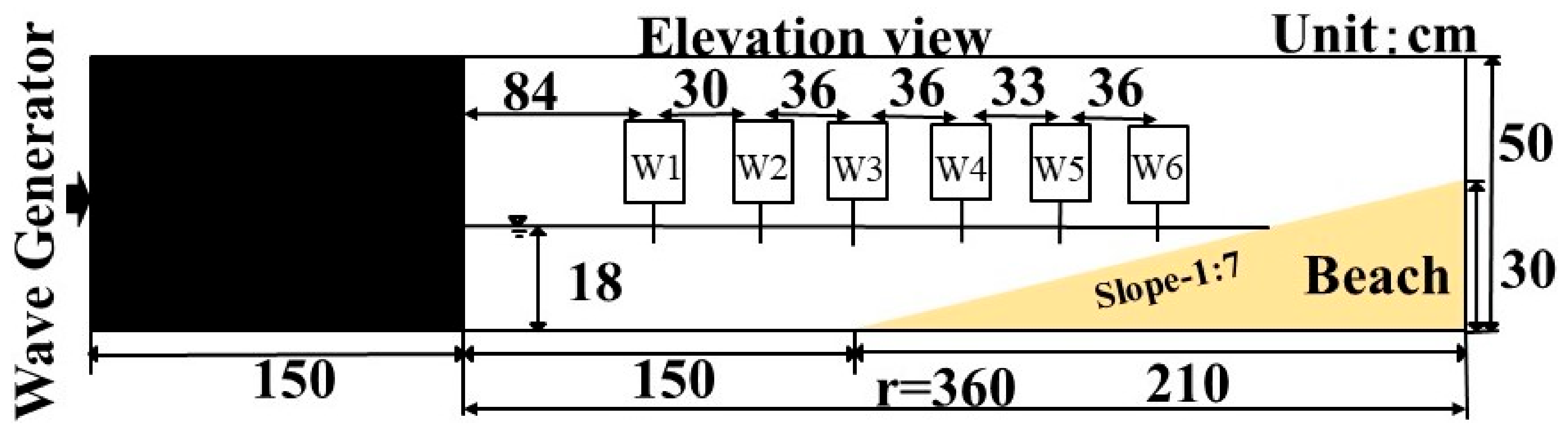
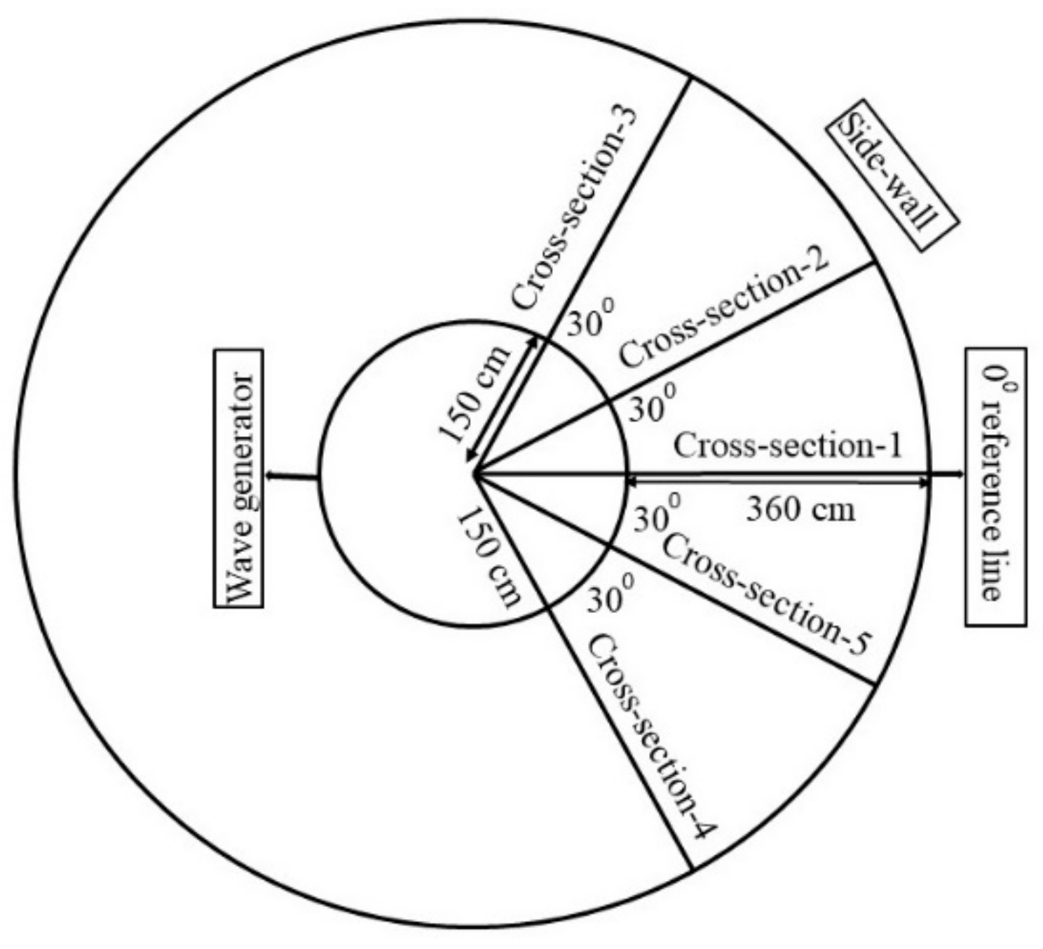
4. Parameters and Experimental Conditions of the Wave Tank Model

4.1. Numerical Calculations

In this study, we subdivided the computational domain of the circular wave tank into $M=5$ blocks following the method proposed by Suh and Yeo [45], which we implemented in the zonal embedded grids method. According to the method, the numbers of grids in each block in the radial, azimuthal, and vertical directions were defined by $I_M=I_0$ ($M=1)$, $I_M=2^{M-1}{I}_0$, $J_M=2^{M-1}{J}_0$, and $K_M=K_0$ for $\left(M\ge 2\right)$, respectively, where $I_0$, $J_0$, and $K_0$ represent the number of grids in the first block. The grid number in each block of the computation domain was different and fixed, where the grid spacing in the radial direction was fixed similar to a regular orthogonal grid system ($\Delta r=0.03 \mathrm{m}$). We reorganized the spacings by halving the previous block in the azimuth direction in the zonal embedded grid system. The vertical grid spacings could be reorganized in any way within the fixed grid number, which we considered as 0.75 cm (1–56) and 1.5 cm (57–88) in the computation. Moreover, we used the high-resolution scheme to accurately track the free surface in the vertical direction. In this numerical model, we fixed the diameter of the numerical wave tank by 10.2 m, corresponding to the radius of the wave generator of 150 cm positioned at the center of the wave tank, which was considered at the sidewall boundary in a previous study [27]. The computational time needed for running a single test case was approximately 5–6 days using a high configuration computer (Processor: Intel Core-i9-9900k CPU @3.6 GHz, RAM: 32 gb (Santa Clara, CA, USA)). The calculation conditions of the grid spacing in the radial, azimuthal, and vertical directions are shown in

Table 1. Grid arrangement in zonal grids in the computational domain.

Zone	M	5
Number of grids in radial direction	1	5
	2–4	5, 10, 20
	5	80
Number of grids in azimuthal direction	1–5	60, 120, 240, 480, 960
Number of grids in vertical direction	1–5	88

.

To observe the spiral wave generation on sloping beach topography, we considered a sloping beach with a ratio of 1:7 in this study. A sectional view of the terrain is shown in Figure 2. We measured the water surface elevations and velocity profiles during the computations with several wave and velocity gauges that were set up in different cross-sections (Figure 3) in different wave conditions on the present sloping numerical circular wave tank. The wave and velocity gauges positions are shown in Figure 2, and the computation conditions are presented in

Table 2. Numerical computation conditions for wave generation.

Cell size	Δr	0.03 m	Total calculation Time		60 s
	Δz	0.75 cm, 1.5 cm	Time step	dt	Max. 0.005 s
Water depth	h	0.18 m	Measured cross-section		5
Wave period	T	1.80 s, 2.0 s, 2.25 s, 2.50 s	Median particle size of the beach	$d_{50}$	0.4 mm
Wave height	H	1.5 m	Nonlinear drag coefficient	$C_{D1}$	0.45
Water density	${\rho }_w$	1000 kg/m3	Linear drag coefficient	$C_{D2}$	25.0
Air density	${\rho }_a$	1.2 kg/m3	Kinematic viscosity of air	${\mu }_a$	1.8 × 10−5 Pa.s
Added mass coefficient	CA	−0.04	Kinematic viscosity of water	${\mu }_w$	1.01 × 10−3 Pa.s

.

4.2. Hydraulic Model Experiment

To clarify the spiral wave generation in the proposed numerical circular wave tank model and compare the numerical and experimental results, we conducted hydraulic experiments on a circular wave tank with a diameter of 10.2 m and height of 0.5 m, the same as the numerical wave tank, which we set-up in the hydraulic experiment laboratory at Nagoya University (Islam et al. [40]), as shown in Figure 4. A non-rotating spiral wave-making device with 16 piston-type wave paddles was positioned at the center of the wave tank, and the wave paddles were connected with a crankshaft, by which the paddles were shifted forward and back to generate oblique waves on a circularly sloping topography without the influence of sidewall edges. We controlled the movement of the paddles with a motor (Model-G3F32N20-MD15TNNTN, Nissei Corporation, Aichi, Japan) connected to the crankshaft paired with an inverter (Yaskawa-J1000, Yaskawa Electric Corporation, Fukuoka, Japan) for controlling the rotational speed of the motor. The outer sidewall was composed of 64 vertical and horizontal vinyl chloride boards. We set up a sloping beach topography with a 1:7 ratio and silica sands with a particle size of approximately 0.4 mm ($d_{50}$) along the outer circumference of the basin.

The wave characteristics, flow velocities, and water surface elevations were measured with an electro-magnetic velocimeter (KENEK: VMT2-200-04PL, Kenek Corporation, Tokyo, Japan) positioned at one point and a capacitance-type wave gauge (KENEK: CHT6-30, Kenek Corporation, Tokyo, Japan) positioned at four points on the measured cross-section in the physical experiment. The experimental conditions are presented in

Table 3. Experimental conditions.

Case	1	2	3	4
Period	1.82 s	2.0 s	2.22 s	2.50 s
Water depth	18 cm
Initial Terrain	1:7 Uniform Slope

. The sand on the beach profile eroded and accreted due to the wave propagation and breaking on the sloping topography during the experiment, which finally changed the topography. Note that we did not consider sand displacement procedures on the sloping topography in this numerical circular wave tank model; however, the velocity profiles and water surface elevations were easily measured at different positions on different cross-sections with this numerical wave tank model, which was comparatively difficult due to the lack of experimental facilities for the physical experiments. The details of the experimental procedures and mechanisms of the wave generation in the physical experiment can be found in Islam et al. [40].

5. Results and Discussion

We implemented the two-phase incompressible flow model described in this paper to simulate spiral wave generation in a numerical circular wave tank. To describe the wave generation procedure and performance of the numerical wave tank model, we performed computations under different wave conditions to demonstrate the generated wave characteristics in several computation cases. The numerical results were compared with the physical experiment results to validate the proposed numerical model.

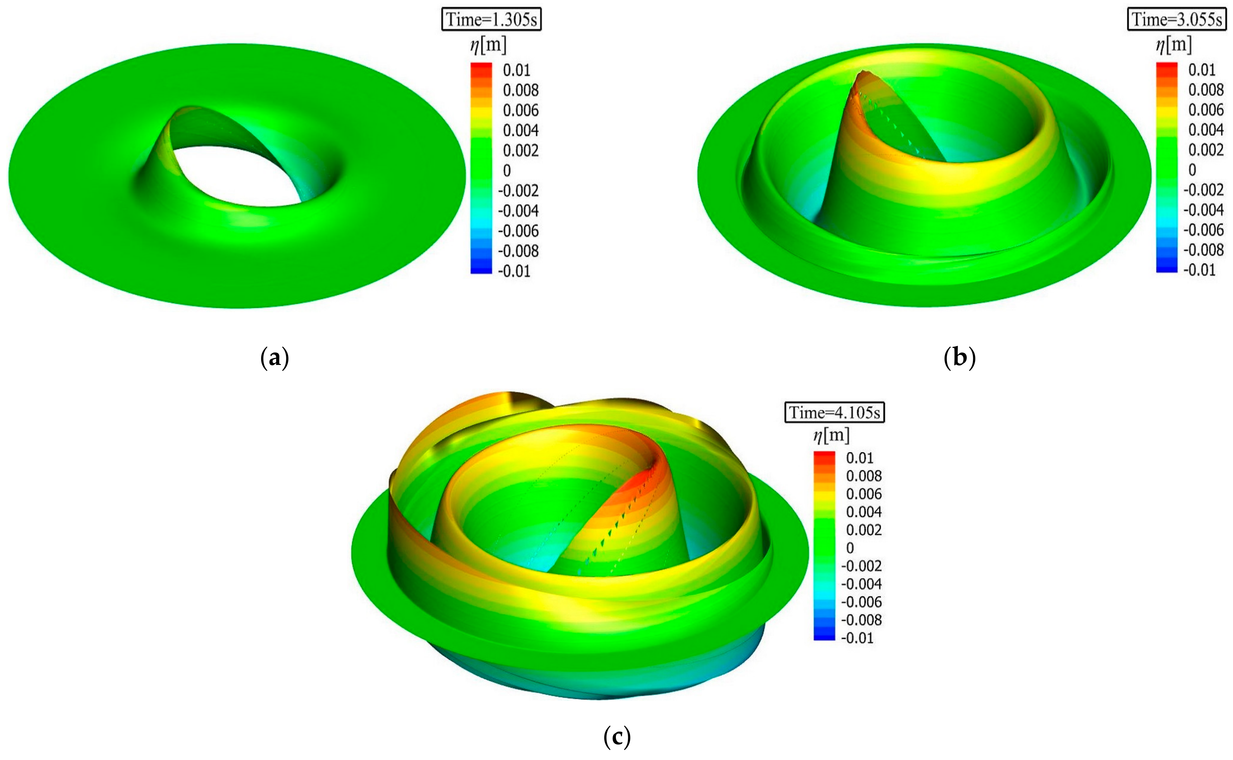
5.1. Spiral Wave Generation

In this study, we added a mass source term to generate spiral waves in the wave tank model. To demonstrate this, we substituted the wave potential by the Airy wave potential into the Equation (2); thus, the discretized mass source term could be written as

$$Q\left(r_s,{\theta }_s,z,t\right)=\frac{2u_r\left(r_s,\theta ,z,t\right)}{\Delta r}\frac{{{\displaystyle \int }}_{-h}^{\eta }{u}_r\left(r_s,\theta ,z,t\right)dz}{{{\displaystyle \sum }}_1^{k_{max}}{u}_r\left(r_s,\theta ,z,t\right)\Delta z}$$

(19)

$$u_r\left(r_s,\theta ,z,t\right)=k\frac{gH}{2\omega }\frac{\cos \mathrm{h} \mathrm{k}\left(h+z\right)}{\cosh kh}\cos (k{r}_s-\omega t-\theta )$$

(20)

where $k_{max}$ is the highest nodal point in the vertical direction of the wave source zone; H is wave height; k is the wave number; $\omega$ is the angular wave frequency; $u_r\left(r_s,\theta ,z,t\right)$ is the velocity of the wave-making source in spiral waves; and $\Delta r$ and $\Delta z$ are the mesh lengths at wave-making point $r_s$ in the r and z direction respectively. In this study, we placed the wave-making source in the central position with a circumferential shape ($\theta =0-2\pi$, incident wave direction) of radius $r_s=150 \mathrm{cm}$. The calculation conditions are shown in Table 2.

To continue wave generation using the above-mentioned wave source function, gradually increase the strength of the wave-making source, and improve the stability, we modified the wave source term (Iwata et al. [54]) in the computation as

$$Q\left(r_s,{\theta }_s,z,t\right)=\left\{\begin{array}{c} 1-\exp \left(-0.5t/T\right)\}.Q\left(r_s,{\theta }_s,z,t\right) ;t/T\le 3\hfill \\ Q\left(r_s,{\theta }_s,z,t\right) ; t/T>3\hfill \end{array}\right.$$

(21)

The values of the resistance coefficients inside the porous media and the added mass coefficient used in this numerical model were $C_{D1}=0.45$, $C_{D2}=25.0$, and $C_A=-0.04$, similar to those used by Mizutani et al. [41].

From the outcomes in each case, we found that the mean water level increased over time; however, the total volume of water in the computational domain should be conserved. To address this situation and follow the conservation law of the equation of continuity, we modified the horizontal flow velocity Equation (20) of the wave source using the Stokes drift adopted by Fujiwara [55] as

$$u_r\left(r_s,\theta ,z,t\right)=k\frac{gH}{2\omega }\frac{\cos \mathrm{h} k\left(h+z\right)}{\cosh kh}\cos (k{r}_s-\omega t-\theta )-C\overline{U}$$

(22)

where $\overline{U}=\frac{1}{2} \frac{k\pi H^2}{2T}\frac{\cosh 2k\left(h+z\right)}{{\sinh }^2\left(kh\right)}$, which is the velocity of the stokes wave; and C is the correction factor, which we calculated by using the Ursell number $U_r=H{L}^2/h^3$ as $C=0.62U_r^{0.08}$. The coefficient of the Ursell number was fixed at 0.62 by Fujiwara [55]; however, it can be calibrated depending on the wave conditions. The Ursell number varied between 0.76, 0.73, and 0.67 in different wave conditions in this study.

We conducted the computations for 60 s in each case. Figure 5 shows the snapshots of the wave generation procedures at different time intervals in this model in the case of T-2.0 s, where contour colors define the differences in water surface levels at the specific time point. The figure shows that the waves were spirally generated (Figure 5a) and moved along the circumference of the wave tank. Additionally, the water surface elevations are shown in Figure 5b,c. Considering the snapshots, we inferred that the spiral waves were generated by using the considered wave source function in the presented numerical circular wave tank model.

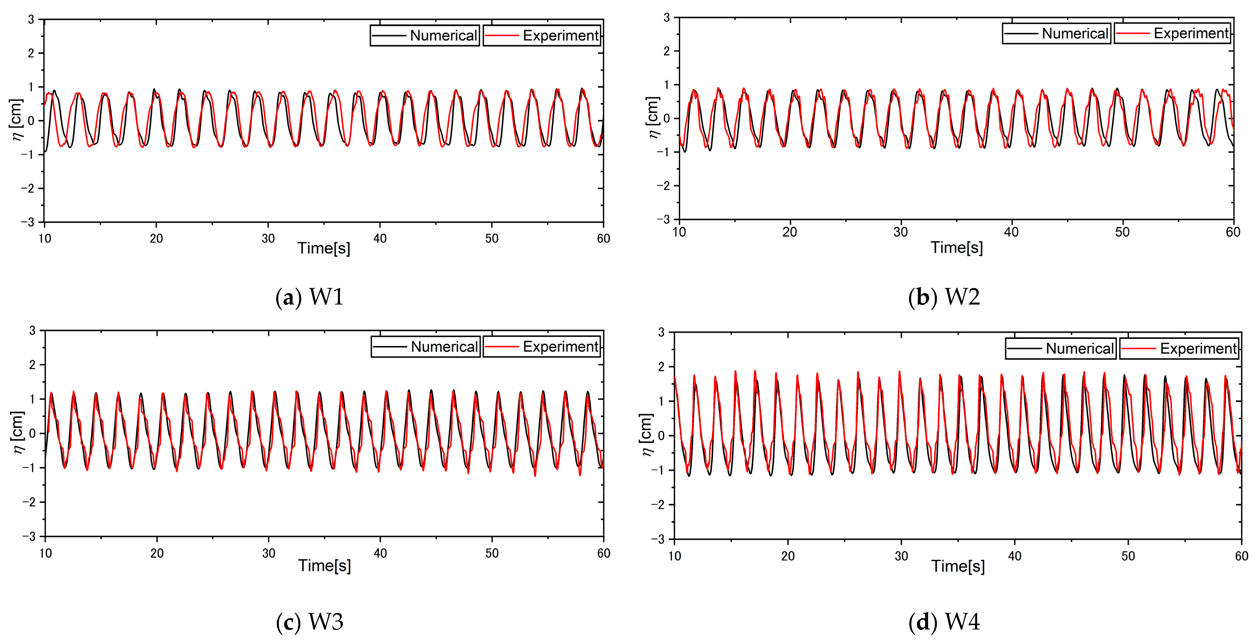
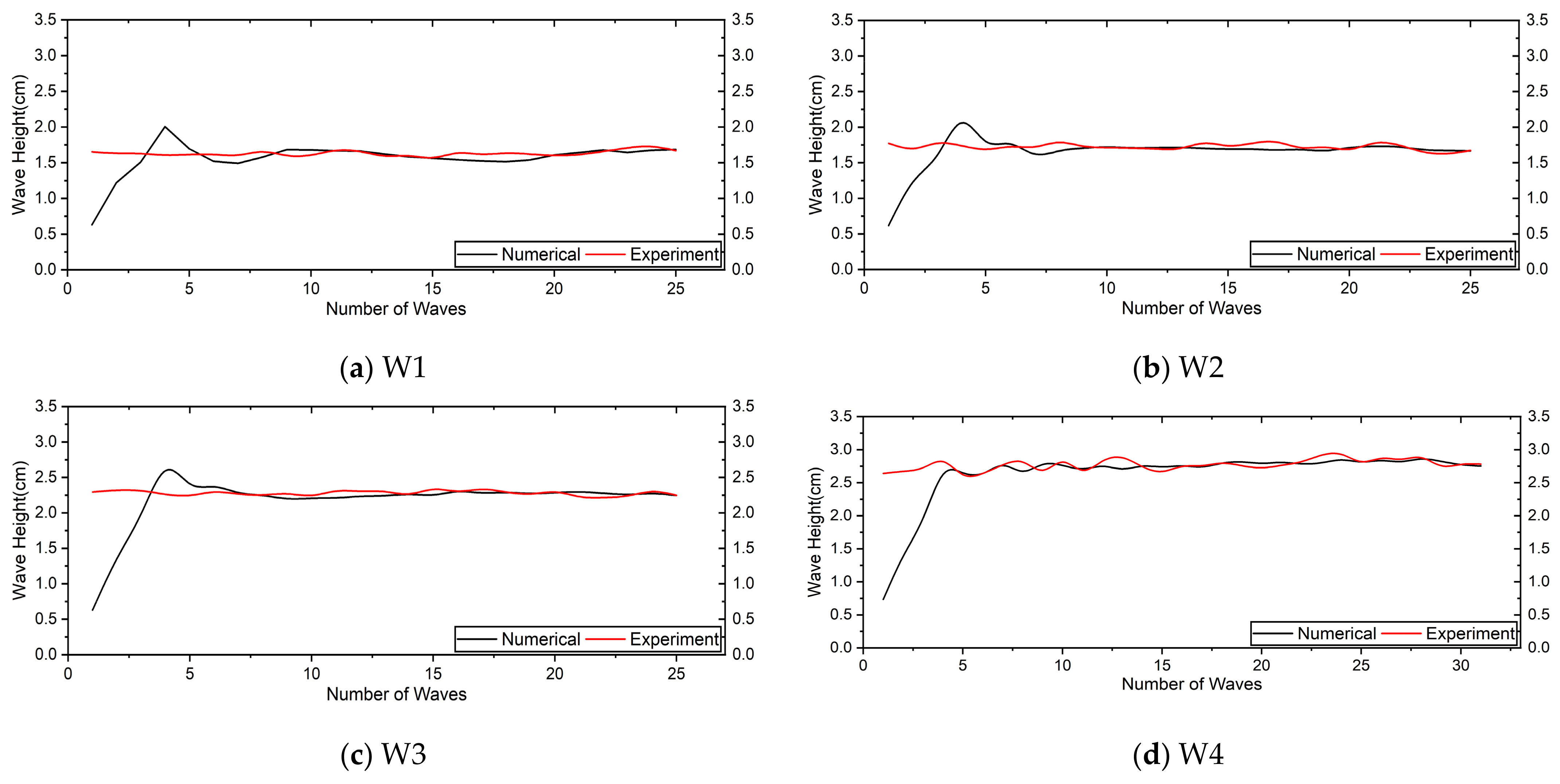
5.2. Model Validation

To demonstrate the performance of the proposed numerical model, we performed numerical calculations using conditions similar to those in the experiment (Islam et al. [40]); the numerical and experimental results were compared. We conducted the physical experiments for 60 min in each case, whereas the computations continued for 60 s. Within the calculated results, the water surface elevation profiles in different wave conditions were considered in both the numerical and experimental cases, as shown in Figure 6. The wave periods of the computed surface elevation profiles at W1, W2, W3, and W4 in Figure 6 are not the same, which means the wave periods of the compared profiles at W3 (T-2.0 s) and W4 (T-1.82 s) measured positions were different from those at W1 and W2 (T-2.22 s). We obtained the results at the corresponding measurement positions in the cross-sections of the wave gauges in the numerical and experimental models.

From the comparison, we observed that the surface elevation profiles were almost the same in the crest and trough positions, showing little difference. Comparing the results at individual positions, the results were markedly different at the crest and trough positions, with magnitudes at W3 and W4. Additionally, the measurement profiles of the experiment at W3 and W4 were not as linear as in the numerical model, which could have occurred due to the influence of returning flows on the deformed topography during the experiment. The comparison of the measured wave heights at different positions in the numerical calculations with experimental results is shown in Figure 7. We found that the wave height at each wave gauge position was almost the same in a line, with small differences at some points. The experimental wave heights in Figure 7 were obtained at different time intervals and compared with the considered experimental results in Figure 6 (i.e., the experimental time intervals considered at W1 in Figure 6 and Figure 7 were not the same) to represent the performance. Since sand was displaced during the physical experiment and the topography changed during the experiment in all experimental cases, sediment transport was not considered in the numerical wave tank model. The discrepancies could have occurred due to the topography changes in the physical experiment, but not in the numerical cases. The influences of sand displacement are shown in Figure 6c,d and Figure 7c,d. The wave generation procedures and the generated wave profiles followed the same pattern in both the experiment and the numerical wave tank models, which we visually observed during the experiment, as shown in Figure 5.

As the water surface elevation profiles and wave heights under different wave conditions and time intervals mostly followed the same pattern as the profiles in both the experiment and numerical wave tank models, we inferred that the proposed model was capable of generating the same spiral waves on a sloping beach topography as in the physical experiment. Additionally, the model can be used for further investigation into obliquely generated wave characteristics and other factors in a sloping circular wave tank model.

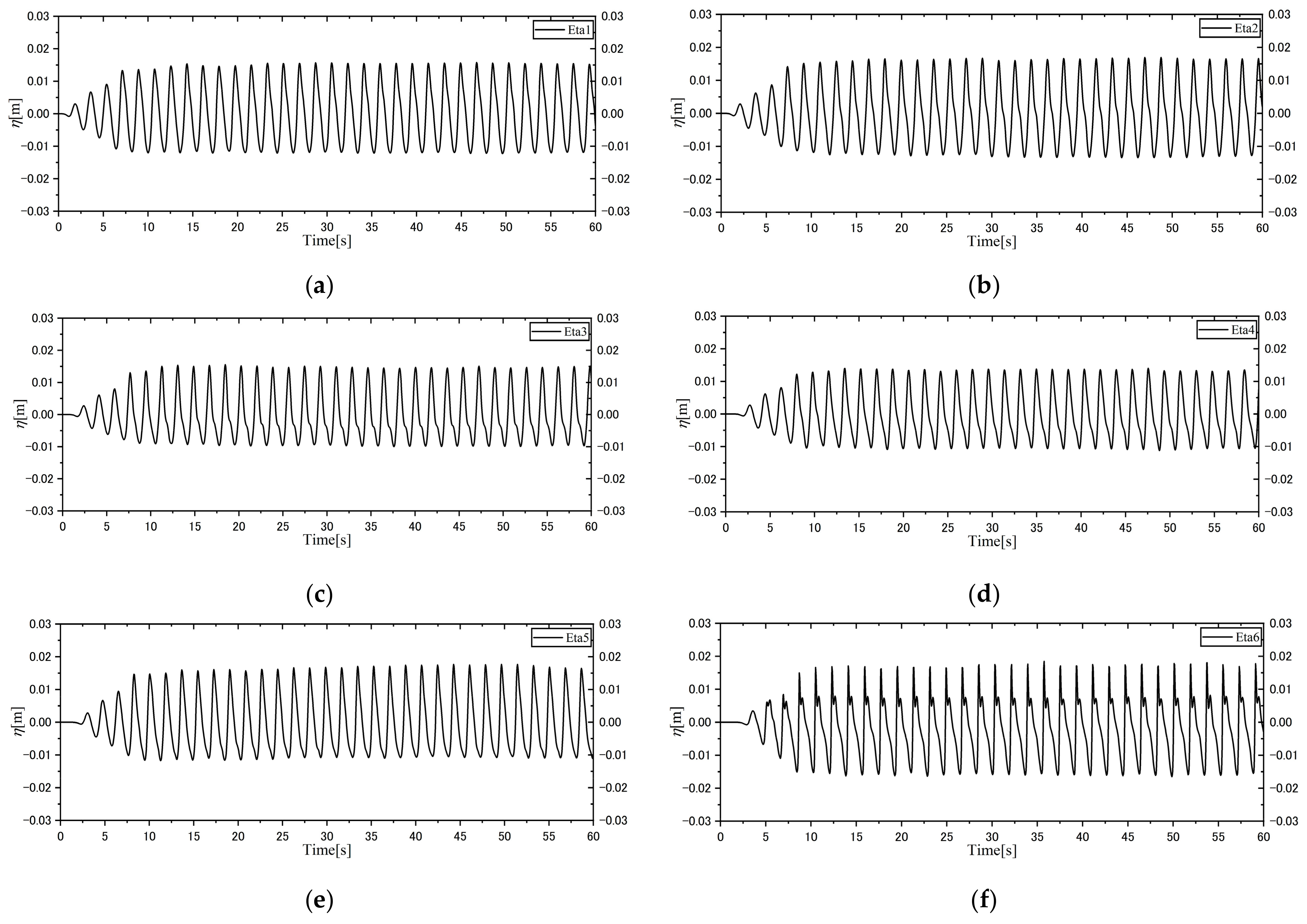
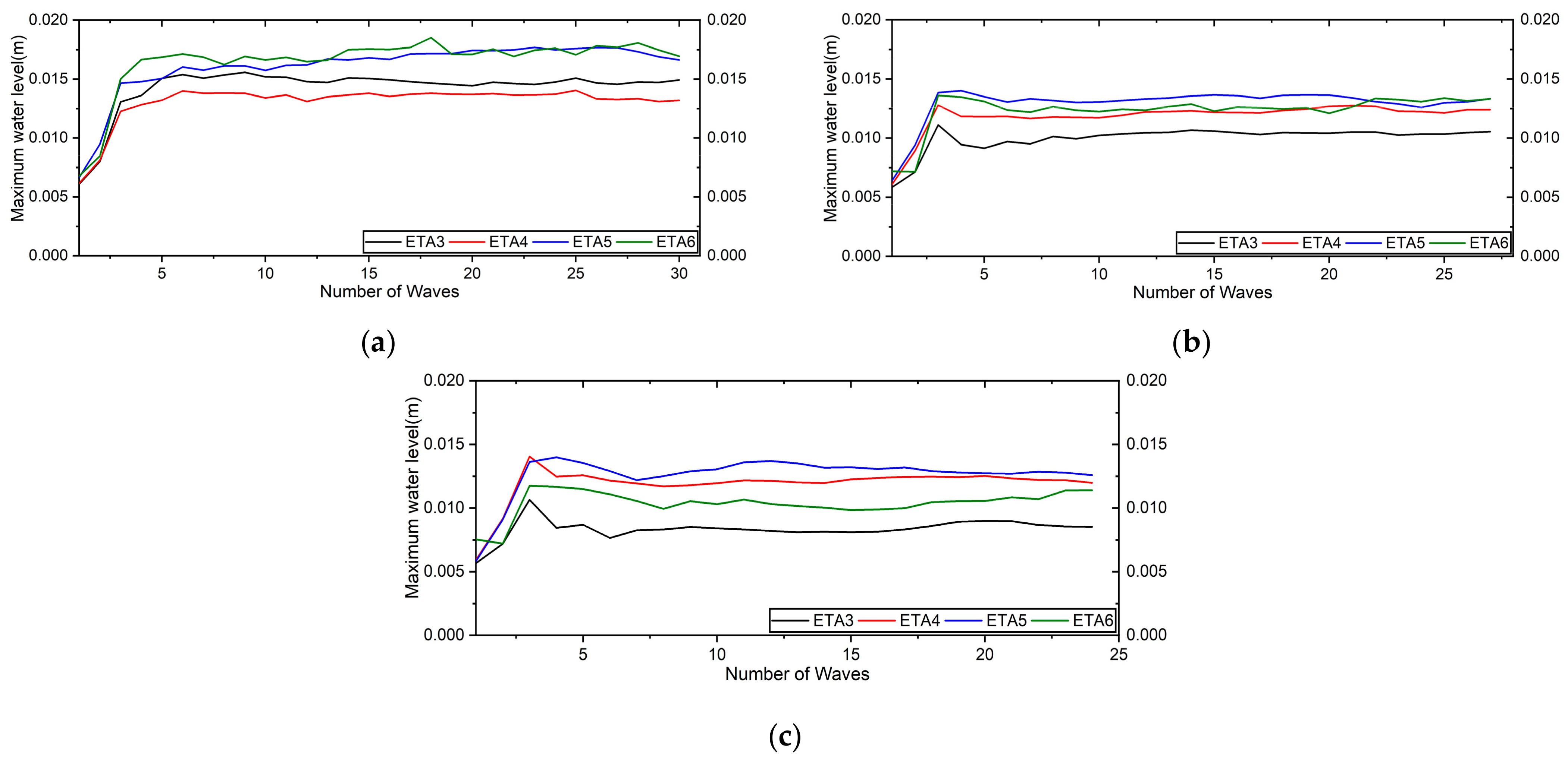
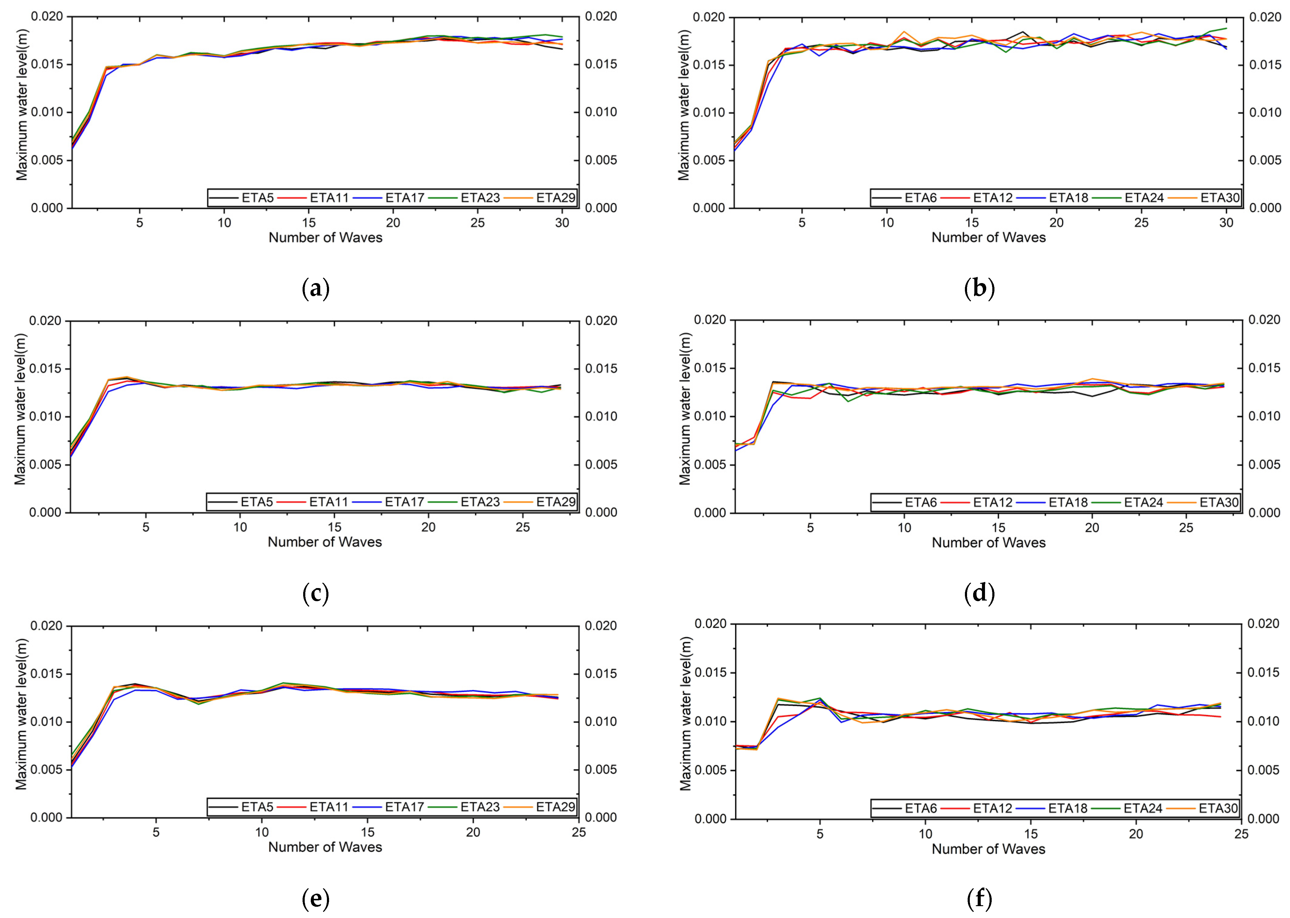
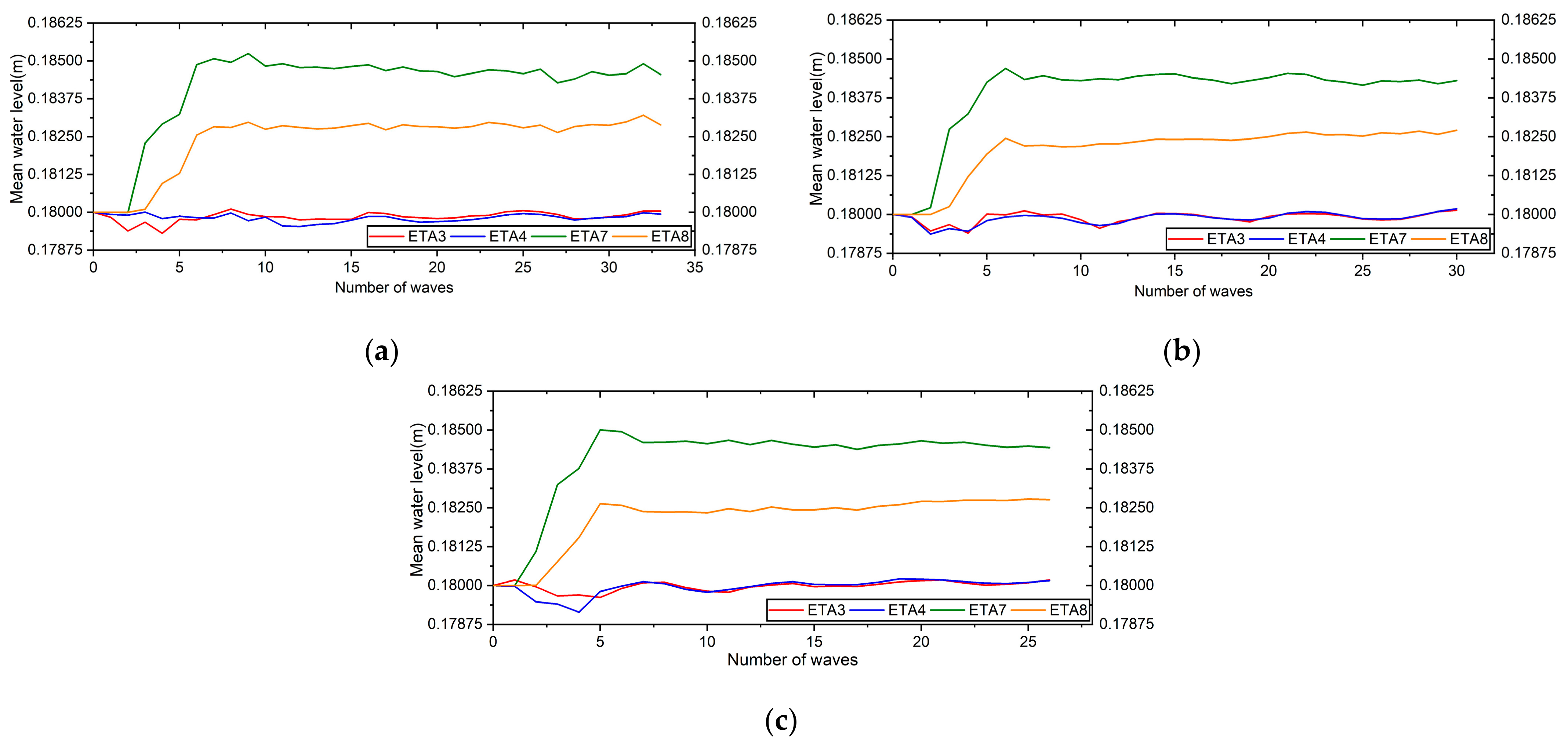
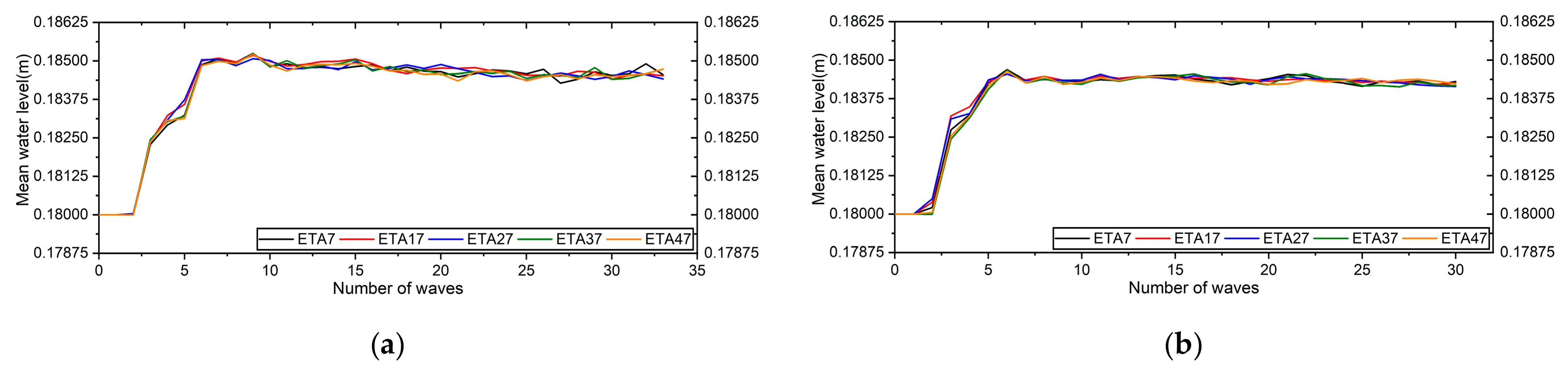
5.3. Wave Characteristics

In this study, we performed the computations under different wave conditions, where a uniform gradient of 1:7 was considered the initial terrain. We investigated the obliquely generated wave characteristics under the four different wave conditions described in Table 2. We measured the water surface fluctuations at different positions in a cross-section; the wave gauges were set up at particular distances from the wave generator in each cross-section. We conducted the computations for 60 s in each case.

Figure 8 shows the water surface fluctuations in cross-section 1 at the W1, W2, W3, W4, W5, and W6 wave gauge positions in case 1, where the still water level was 0 cm and the measured water surface fluctuations were denoted by Eta 1 to Eta 6, respectively. From the outcomes in each case, we observed that the magnitudes of the water surface fluctuations tended to increase over time. This tendency was particularly observed at wave gauge positions that were closer to the wave maker, and the magnitudes gradually decreased at other measured wave gauges compared with the closest measured positions. Moreover, the magnitudes increased again at the wave gauges that were placed at a more shoreside location due to the wave deformation in the shallow water depth in each case. The differences in water surface fluctuations are shown in Figure 8. From this figure, we found that the magnitudes were higher at Eta 1 and Eta 2 than to Eta 3 and Eta 4, as Eta 1 and Eta 2 were closer to the wave maker, and then increased again at Eta 5 and Eta 6, which were positioned nearest the shoreside in case 1 (T-1.80 s). Similar increasing and decreasing trends were also found in other cases (T-2.0 s, 2.25 s, and 2.50 s). In addition, the magnitudes of the measured surface fluctuation profiles in different wave period cases were different, and the values of magnitudes were high in the T-1.80 s case compared with the others. The wave period correlated with the movement of the wave generator, and the movement of the wave generator was faster per second in this case (T-1.80 s), which could be one of the reasons for the higher surface fluctuation magnitudes at the measured positions in the same angular cross-sections compared to under other wave conditions.

The maximum water levels per wave (crest position) at the measured wave gauge positions were also different at W4, W5, and W6 positions in all cases. Individual values were high from W4 to W6 or sometimes fluctuated between the two of them under different wave conditions in the same sloping case, which indicated that the waves were breaking at the positions where the crest position was higher in a single case during the computation. In addition, the mean water level was lower at the positions where the waves broke in the studied cases. This finding is similar to those of theoretical studies of wave breaking on a sloping beach profile. Comparing the measured maximum water level profiles in case 1, we found that the maximum water level per wave was higher between W5 and W6 in this case. However, the value was mostly higher at W6 than at W5 for most of the waves, which can be observed in Figure 9a. Additionally, the mean water level was lower at W6 than at W5 per wave during the whole computation. These findings indicated that the waves were breaking in the vicinity of W6 in this case. A similar finding was obtained at other measured cross-sections in this case.

The maximum water levels per wave were higher mostly at W5 and a little higher at W6 for some waves in case 2. The levels were substantially higher at W5 in case 3 and fluctuated between W4 and W5 in case 4. The comparisons of cases 2 to 3 are shown in Figure 9b,c, and the profiles indicate that the waves approximately broke in the vicinity of W5 in case 3, between W5 and W6 in case 2, and between W4 and W5 in case 4. The variations in the maximum water levels per wave in single cases in the same measured cross-section 1 indicated that the wave-breaking positions differed under the different wave conditions in a fixed-slope topography.

5.4. Comparisons for Different Conditions

To observe the differences in water surface elevation profiles and wave-break positions in different cross-sections in each case, we recorded measurements from five different cross-sections with 30° differences (0°, 30°, 60°, 300°, and 330°) from each other in each case. The cross-section positions are shown in Figure 3. From the computational results, we observed that the wave heights, maximum water levels, and mean water levels differed and followed the same trends as in the above-discussed cross-section 1 in each case. These three components differed at the same radial distances in different cross-sections under the same wave condition. Furthermore, the maximum water levels per wave at the same radial distances in the above-mentioned different cross-sections were not the same as in individual cases. The variations in cases 1, 2, and 3 at wave gauges W5 and W6 are shown in Figure 10. The measured water levels at the radial distance of 369 cm in different cross-sections (1–5) were defined as Eta 5, Eta 11, Eta 17, Eta 23, and Eta 29, respectively, and at the distance of 405 cm by Eta 6, Eta 12, Eta 18, Eta 24, and Eta 30, respectively.

The profile differences of the maximum water levels in each case (Figure 10) indicated that the wave-breaking positions were not the same at the same radial distances from the wave maker in a single wave condition. The gradient of the water level differences was one of the reasons for the discrepancies during the computation. We also found that the changes in the ratios of the maximum water level profiles were comparatively higher in case 1, as shown in Figure 10. The variations could have occurred because the number of rotations during the whole computation and the magnitudes of the water surface elevations in all measured positions were higher in this case than in the others. This finding indicated that the wave-breaking position differences at the same radial distances in different cross-sections correlated with the wave periods on the same sloping topography. Similar wave-breaking position differences were observed in the physical experiment, and the breaking positions were identified by the bars generated throughout the sand accretion and erosion on the beach topography during the experiment. We also visually observed that the generated bar positions and wave-breaking positions were almost the same, and the bar profiles were curved in shape at different radial distances in the topography; however, the approximate breaking positions were not calculated due to the lack of wave gauges during the experiment (Islam et al. [40]).

We considered the mean water levels at the measured positions of cross-section 1 in the four cases to determine the wave set-up in each case in this study. From the outcomes, we found that the mean water level per wave was higher at the wave gauges at 426 cm (Eta 7), which was a little lower at 432 cm (Eta 8) in all cases. The computed results are shown in Figure 11, from which we inferred that the calculated profile of Eta 7 was the wave setup values per wave in each case during the computation in this study. In addition, we computed the mean water level at the same distances in different five cross-sections (Figure 3); the outcomes from cases 1 and 2 were presented in Figure 12. Eta 7, Eta 17, Eta 27, Eta 37, and Eta 47 indicate the measurement data at $r=426 \mathrm{cm}$ at cross-sections 1–5, respectively. The wave set-up values per wave differed on the different cross-sections in both cases; the differences could have occurred due to the wave-breaking positions in each considered cross-section in a single case. Similar outcomes were found in cases 3 and 4, indicating that the wave-breaking positions differed at the same radial distances in a single case during the computation on the sloping topography.

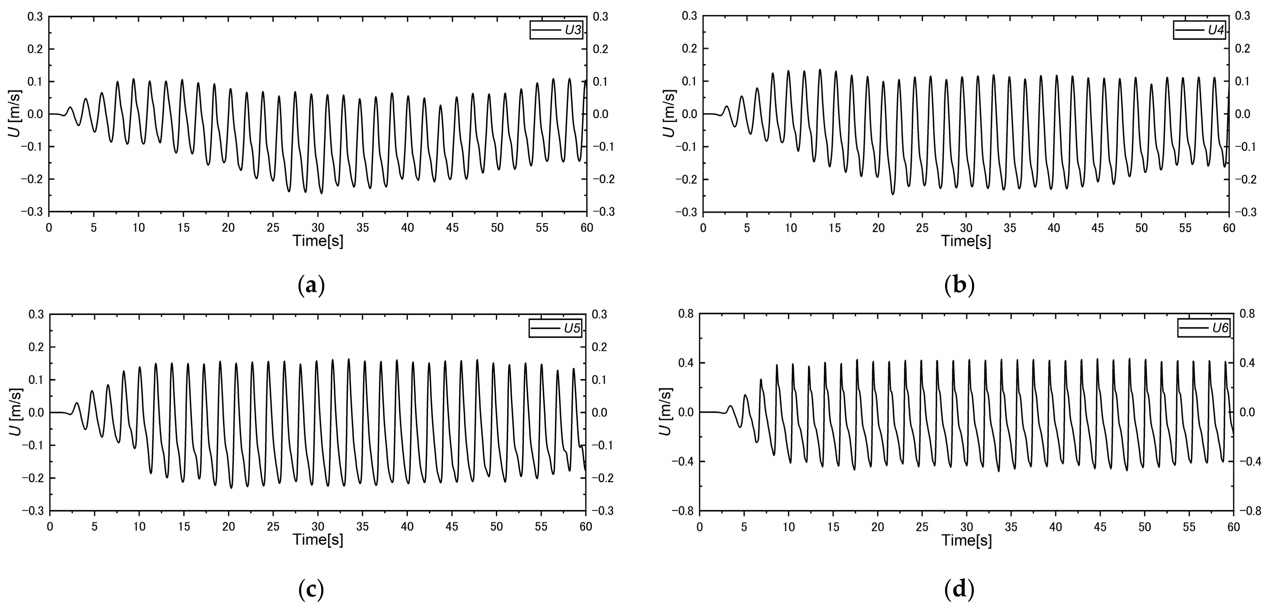
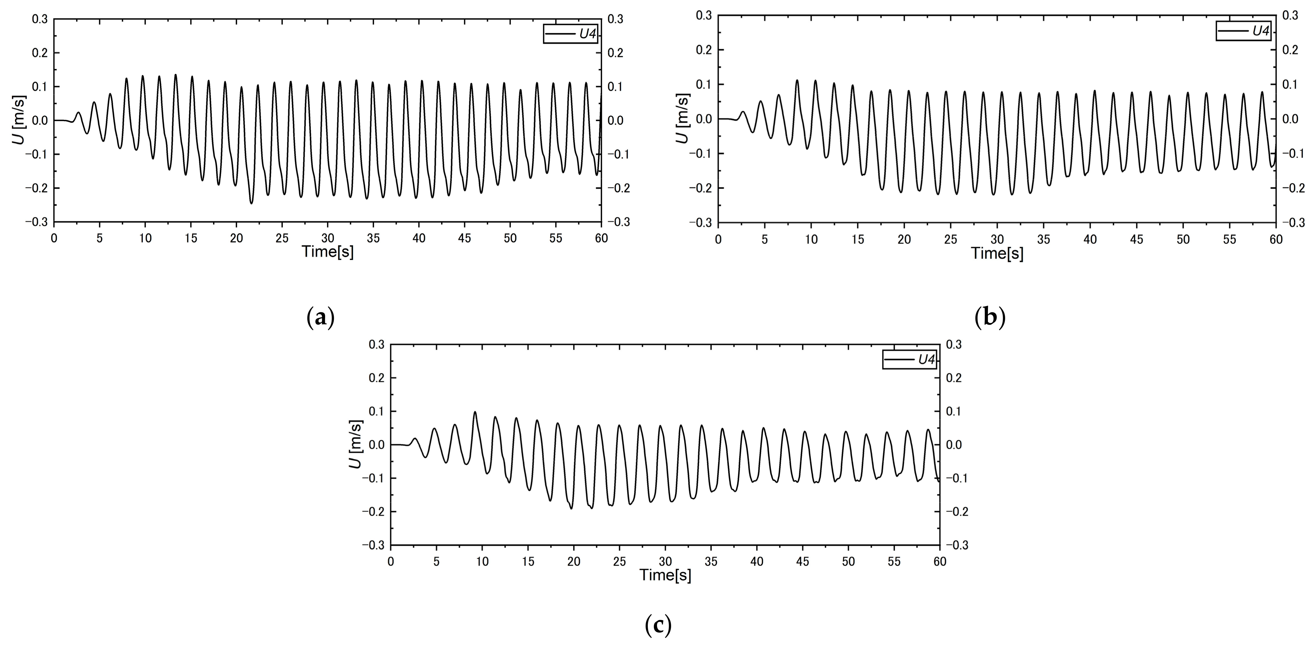
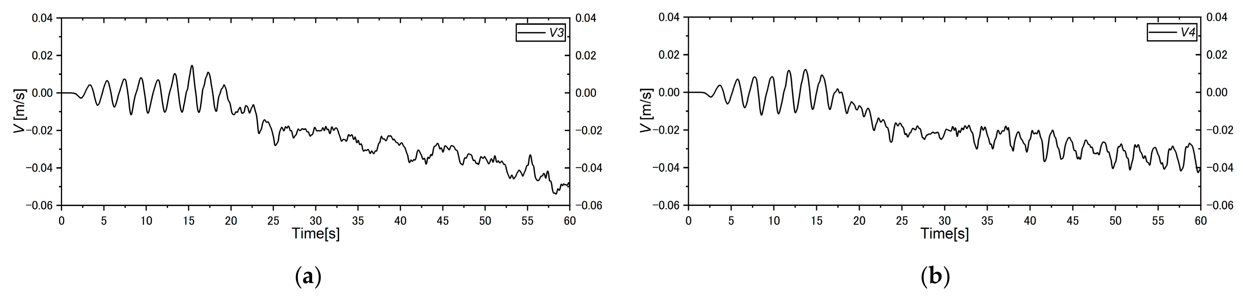
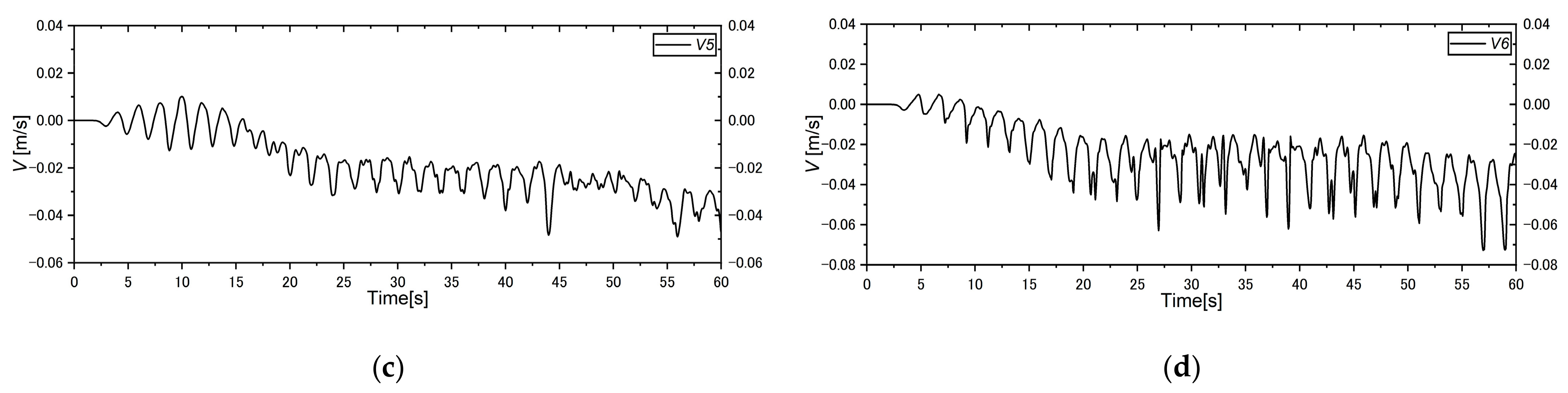
5.5. Cross-Shore and Longshore Velocity Distribution

In addition to the water surface fluctuations, we computed the velocity profiles using the data from the velocity gauges set at the same positions as the wave gauges in all the computation cases. Figure 13 shows the cross-shore velocity ($U$) profiles at U3, U4, U5, and U6 in case 1 (T-1.80 s), which were positioned at the same cross-sections (cross-section 1) as wave gauges W3, W4, W5, and W6, respectively, on the sloping topography. From the outcomes, we observed that the cross-shore flow velocity was consistently generated in all cases and that the velocity profiles were linearly formed from the start of the experiment in cross-section 1. The magnitudes of the flow velocity increased over time, and the magnitudes were remarkably increased in case 1 (T-1.80 s) compared with the others, as the rotational speed of the wave maker was higher in this case. In addition, the velocity profiles at the measured locations did not follow the same pattern as in the total computation; the profiles were varied due to their measurement positions. During the computation, the flow velocities at U3 (300 cm) and U4 (336 cm) decreased after a while under the influence of the obliquely generated breaking-wave direction and downstream flow, then stably moved again until the end of the computation in all cases. Flow velocity was mostly stable at U5 (369 cm) and U6 (405 cm) from the start of the experiment. Additionally, the influence of upstream flow was strong compared with that of downstream flow along the onshore and offshore directions, which were remarkably observed at U3 and U4 in all cases.

Considering the measured cross-shore flow velocities in individual cases, we found the velocity profile movement along the direction of rotation in an earlier stage at U3 in case 1 (T-1.80 s) than in the others. The movements started approximately after 15, 17, 18 and 20 s respectively in cases 1–4, respectively, at U3. The flow velocity steadily moved again, following the onshore direction, after 30–35 s in this measured position in individual cases. The influence of the direction of rotation on the flow velocity at U4 was not as strong as the one found at U3. The velocity steadily moved in the onshore direction earlier in case 1 than in the others, which can be confirmed by Figure 14. The velocity profiles along with the influence of the upstream and downstream flow were strong and stable at U5 and U6 in all cases; this phenomenon was remarkably observed in case 1. Additionally, the magnitudes were higher in case 1 than in the others. We found similar characteristics of the cross-shore flow velocity in other measured cross-sections in individual cases, indicating that uniform wave generation could have occurred during the computations in all cases of this numerical circular wave tank model.

The longshore flow velocity ($V$) waveform was almost symmetrical after the start of computation, and the velocity in the following and opposite direction of rotation was also found in all cases. Figure 15 shows the longshore velocity measurement at V3, V4, V5, and V6 in case 2, where the velocity gauges were positioned at the same cross-section and positions as wave gauges W3, W4, W5, and W6, respectively. The flow velocity components along the direction of rotation (negative component) were remarkable in case 1, where the rotation speed of the wave generator was higher compared to that in the other cases. The mentioned characteristics found earlier at V4, V5, and V6 compared with those of others in Figure 15. Longshore flow velocity was dominant after 15, 17, 18, and 20 s at V4 and after 14, 15, 16, and 19 s at V5 in cases 1–4, respectively. We observed that the velocity component in the alongshore direction at the considered positions (V3 to V6) followed the breaking-wave directions and the influence of downstream flow in the computational cases. The differences could be understood from the measured velocity profiles at V4 and V5 in case 2, as shown in Figure 15.

From this figure, we found that the velocity considerably moved along the alongshore direction at V4 and V5, and mostly at V5 in case 2 compared with in case 1, which could have occurred due to the wave breaking approximately nearest to the V5 (369 cm) position, as discussed in the above sections. The downstream flow was dominant in the vicinity of the V3 and V4 positions in case 2. The waves were approximately broken in the vicinity of the V6 measurement position in case 1; the longshore velocity was remarkably dominant at V5 and V6, and the downstream flow was dominant in the vicinity of the V4 and V5 measurement positions in this case. Additionally, we found the velocity in the opposite direction of rotation at V3 and V4 in case 3, which indicated that the downstream flow moved in the negative direction in this case. The longshore flow velocity in the alongshore direction was not dominant in case 4, and the velocity profiles remarkably fluctuated at all velocity gauges in case 4.

From the above discussion, we concluded that the wave-breaking positions were not the same in each case and that a time lag occurred with wave-breaking on a sloping topography during the computation. The incident wave heights, wave periods, wave-breaking positions, and downstream flow strongly influenced the cross-shore and longshore velocity distributions. Longshore current could be generated and act as the wave-driving force during the computation in this numerical wave tank, which we considered to be responsible for the deformation of the beach profile during the experiments in a physical circular wave tank. Further investigation is needed to fully understand the mechanisms of the longshore current generation.

6. Conclusions

In this study, we introduced a circular wave basin model with a two-phase incompressible flow model in 3D cylindrical coordinates, where we discretized the governing equations by a finite volume method, and we tracked the free surface between the air and water with the volume of fluid method. To consider a large diameter computational domain and obtain a grid-independent solution in the computational area, we adopted a zonal embedded grid system in this model, and we added a mass source function to the continuity equation to reproduce oblique waves with a spiral wave generator positioned in the center of the wave tank. We used a high-resolution scheme (CICSAM), a projection method, and the AGMG method to solve the Navier–Stokes equation. We considered a permeable circumferential sloping beach (1:7) along the circumference of the wave basin to investigate wave propagation and other characteristics as on a natural sandy permeable beach profile. To verify the performance of the wave generation procedures, we compared the computed results with the experimental results [40], applying the same wave conditions. The results showed good agreement with the experiment in terms of randomly selected water surface elevation profiles and wave heights under the same wave and sloping conditions. We also observed that the proposed numerical wave generator can reproduce the spiral waves as reproduced by the physical wave maker in the experiment. The numerical results demonstrated that the wave-breaking positions differed under different wave conditions and for different measured cross-sections in a single case. In addition, the wave setup differed in different wave conditions for the same sloping topography; this variation indicated a relationship with wave periods and wave-breaking positions at the same radial distances within a single case. We found a discrepancy in the cross-shore and longshore velocity distribution in different wave periods due to the variation in incident wave heights, downstream flow, and wave-breaking positions on the same sloping beach. This variation indicated that the longshore current could be generated in the present circular wave-making tank. Notably, we assumed that the flows were laminar for all the test cases in this model; a turbulent model can be incorporated into the model to observe the surface flow generation in the circular wave tank in the future. Furthermore, this model can be used for further investigations into the mechanisms of the wave-breaking and longshore current generation for different wave and sloping conditions. Additionally, the influence of beach slope on wave-breaking positions and longshore current generation on a sloping topography may be studied. Moreover, sand displacement terms can be included to investigate the processes of longshore sediment transport and beach deformation on a sandy natural beach and to propose further steps to combat beach erosion.

References

1. Sunamura, T.; Horikawa, K. Two Dimensional Beach Transformation Due to Waves. In Proceedings of the 14th International Conference on Coastal Engineering, Copenhagen, Denmark, 24–28 June 1974; American Society of Civil Engineers: Reston, VA, USA, 1974; pp. 920–938. [Google Scholar] [CrossRef]
2. Kobayashi, N. Analytical Solution for Dune Erosion by Storms. J. Waterw. Port Coast. Ocean Eng. 1987, 113, 401–418. [Google Scholar] [CrossRef]
3. Günaydin, K.; Kabdasli, M.S. Characteristics of coastal erosion geometry under regular and irregular waves. Ocean Eng. 2003, 30, 1579–1593. [Google Scholar] [CrossRef]
4. Kobayashi, N.; Lawrence, A.R. Cross-shore sediment transport under breaking solitary waves. J. Geophys. Res. Oceans 2004, 109, C03047. [Google Scholar] [CrossRef]
5. Eichentopf, S.; Cáceres, I.; Alsina, J.M. Breaker bar morpho dynamics under erosive and accretive wave conditions in large-scale experiments. Coast. Eng. 2018, 138, 36–48. [Google Scholar] [CrossRef]
6. Othman, I.K.; Baldock, T.E.; Callaghan, D.P. Measurement and modelling of the influence of grain size and pressure gradient on swash uprush sediment transport. Coast. Eng. 2014, 83, 1–14. [Google Scholar] [CrossRef]
7. Mizuguchi, M.; Horikawa, K. Experimental Study on Longshore Current Velocity Distribution. Bull. Fac. Sci. Eng. 1978, 21, 123–149. [Google Scholar]
8. Visser, P.J. Laboratory measurements of uniform longshore currents. Coast. Eng. 1991, 15, 563–593. [Google Scholar] [CrossRef]
9. Liangduo, S.; Qinqin, G.; Zhili, Z.; Lulu, H.; Wei, C.; Mingtao, J. Experimental study and numerical simulation of mean longshore current for mild slope. Wave Motion 2020, 99, 102651. [Google Scholar] [CrossRef]
10. Multer, R.H. Exact nonlinear model of wave generator. J. Hydraul. Divis. ASCE 1973, 1, 31–47. [Google Scholar] [CrossRef]
11. Nakayama, T. Boundary element analysis of nonlinear water wave problems. Int. J. Numer. Methods Eng. 1983, 19, 953–970. [Google Scholar] [CrossRef]
12. Lee, J.F.; Leonard, J.W. A time-dependent radiation condition for transient wave-structure interactions. Ocean Eng. 1987, 14, 469–488. [Google Scholar] [CrossRef]
13. Lee, J.F.; Kuo, J.R.; Lee, C.P. The Transient Wavemaker Theory. J. Hydraul. Res. 1989, 27, 651–663. [Google Scholar] [CrossRef]
14. Williams, A.N.; Crull, W.W. Simulation of directional waves in a numerical basin by a desingularized integral equation approach. Ocean Eng. 2000, 27, 603–624. [Google Scholar] [CrossRef]
15. Shih, R.S.; Chou, C.R.; Weng, W.K. Numerical modelling of 3D oblique waves by L-type multiple directional wave generator. In Proceedings of the 19th International Offshore and Polar Engineering Conference, Osaka, Japan, 21–26 July 2009; ISOPE: Mountain View, CA, USA, 2009; Volume 3, pp. 918–925. [Google Scholar]
16. Park, J.C.; Kim, M.H.; Miyata, H.; Chun, H.H. Fully nonlinear numerical wave tank (NWT) simulations and wave run-up prediction around 3-D structures. Ocean Eng. 2003, 30, 1969–1996. [Google Scholar] [CrossRef]
17. Park, J.C.; Uno, Y.; Sato, T.; Miyata, H.; Chun, H.H. Numerical reproduction of fully nonlinear multi-directional waves by a viscous 3D numerical tank. Ocean Eng. 2004, 31, 1549–1565. [Google Scholar] [CrossRef]
18. Li, S.; Shibayama, T. Calculation of wave-induced longshore current in surf zone by using Boussinesq equations. In Proceedings of the 27th International Conference on Coastal Engineering (ICCE), Sydney, Australia, 16–21 July 2000; American Society of Civil Engineers: Reston, VA, USA, 2001; pp. 334–345. [Google Scholar] [CrossRef]
19. Larsen, J.; Dancy, H. Open boundaries in short wave simulations a new approach. Coast. Eng. 1983, 7, 285–297. [Google Scholar] [CrossRef]
20. Israeli, M.; Orszag, S.A. Approximation of radiation boundary conditions. J. Comp. Phys. 1981, 41, 115–135. [Google Scholar] [CrossRef]
21. Lin, P.Z.; Liu, P.L.F. Internal wave-maker for Navier–Stokes equations models. J. Waterw. Port Coast. Ocean Eng. 1999, 125, 207–215. [Google Scholar] [CrossRef]
22. Choi, J.; Sung, B.Y. Numerical simulations using momentum source wave-maker applied to RANS equation model. Coast. Eng. 2009, 56, 1043–1060. [Google Scholar] [CrossRef]
23. Brorsen, M.; Larsen, J. Source generation of nonlinear gravity waves with the boundary integral equation method. Coast. Eng. 1987, 11, 93–113. [Google Scholar] [CrossRef]
24. Ohyama, T.; Nadaoka, K. Development of a numerical wave tank for analysis of nonlinear and irregular wavefield. Fluid Dyn. Res. 1991, 8, 231–251. [Google Scholar] [CrossRef]
25. Tanaka, M.; Ohyama, T.; Kiyokawa, T.; Nadaoka, K. Non-reflective multidirectional wave generation by source method. In Proceedings of the 24th International Conference on Coastal Engineering, Kobe, Japan, 23–28 October 1994; American Society of Civil Engineers: Reston, VA, USA, 1994; pp. 650–664. [Google Scholar] [CrossRef]
26. Naito, S. Wave generation and absorption theory and application. In Proceedings of the 16th International Offshore and Polar Engineering Conference, San Francisco, CA, USA, 28 May–2 June 2006; ISOPE: Mountain View, CA, USA, 2006; Volume 2, pp. 81–89. [Google Scholar]
27. Ren, X.; Mizutani, N.; Nakamura, T. Development of a numerical circular wave basin based on the two-phase incompressible flow model. Ocean Eng. 2015, 101, 93–100. [Google Scholar] [CrossRef]
28. Ren, X.; Gao, Y.; Mizutani, N. Application of the numerical circular wave tank on the simulations of the oblique and multi-directional waves. J. Mar. Sci. Technol. 2015, 20, 711–721. [Google Scholar] [CrossRef]
29. Hirt, C.W.; Nichols, B.D. Volume of fluid (VOF) method for the dynamics of free boundaries. J. Comput. Phys. 1981, 39, 201–225. [Google Scholar] [CrossRef]
30. Harlow, F.; Welch, J.E. Numerical calculation of time-dependent viscous incompressible flow of fluid with free surface. Phys. Fluid 1965, 8, 2182–2189. [Google Scholar] [CrossRef]
31. Osher, S.; Sethian, J.A. Fronts propagating with curvature-dependent speed: Algorithms based on Hamilton-Jacobi formulation. J. Comput. Phys. 1988, 79, 12–49. [Google Scholar] [CrossRef]
32. Austin, D.I.; Schlueter, R.S. A numerical model of wave breaking breakwater interactions. In Proceedings of the 18th International Conference on Coastal Engineering, Cape Town, South Africa, 14–19 November 1982; American Society of Civil Engineers: Reston, VA, USA, 1982; Volume 3, pp. 2079–2096. [Google Scholar] [CrossRef]
33. Nichols, B.D.; Hirt, C.W.; Hotchkiss, R.S. SOLA-VOF: A Solution Algorithm for Transient Fluid Flow with Multiple Free Boundaries; Report LA-8355; Los Alamos National Lab (LANL): Los Alamos, NM, USA, 1980. [CrossRef]
34. Iwata, K.; Kawasaki, K.; Kim, D.S. Breaking limit, breaking and post-breaking wave deformation due to submerged structures. In Proceedings of the 25th International Conference on Coastal Engineering, Orlando, FL, USA, 2–6 September 1996; American Society of Civil Engineers: Reston, VA, USA, 1997; Volume 3, pp. 2338–2351. [Google Scholar] [CrossRef]
35. Dalrymple, R.A.; Dean, R.G. The spiral wavemaker for littoral drift studies. In Proceedings of the 13th International Conference on Coastal Engineering, Vancouver, BC, Canada, 10–14 July 1972; American Society of Civil Engineers: Reston, VA, USA, 1972; pp. 689–705. [Google Scholar] [CrossRef]
36. Mei, C.C. Shoaling of spiral waves in a circular basin. J. Geophys. Res. 1973, 78, 977–980. [Google Scholar] [CrossRef]
37. Trowbridge, J.; Dalrymple, R.A.; Suh, K. A simplified second-order solution for a spiral wave maker. J. Geophys. Res. Oceans 1986, 91, 11783–11789. [Google Scholar] [CrossRef]
38. Williams, A.N.; McDougal, W.G. Hydrodynamic analysis of variable draft spiral wavemaker. Ocean Eng. 1989, 16, 401–410. [Google Scholar] [CrossRef]
39. Suh, K.; Dalrymple, R.A. Offshore Breakwaters in Laboratory and Field. J. Waterw. Port Coast. Ocean Eng. 1987, 113, 105–121. [Google Scholar] [CrossRef]
40. Islam, M.S.; Akita, N.; Nakamura, T.; Cho, Y.-H.; Mizutani, N. Experimental Investigation on the Mechanism of Longshore Sediment Transport Using a Circular Wave Basin. J. Mar. Sci. Eng. 2022, 10, 1189. [Google Scholar] [CrossRef]
41. Mizutani, N.; McDougal, W.; Mostafa, A. BEM-FEM combined analysis of nonlinear interaction between wave and submerged breakwater. In Proceedings of the 25th International Conference on Coastal Engineering, Orlando, FL, USA, 2–6 September 1996; American Society of Civil Engineers: Reston, VA, USA, 1996; Volume 1, pp. 2377–2390. [Google Scholar] [CrossRef]
42. Nakamura, T.; Mizutani, N. Numerical simulation of wind-induced drift behavior of shipping container floating on water surface using three-dimensional coupled fluid-structure-sediment interaction model. In Proceedings of the 26th Symposium on Computational Fluid Dynamics, Tokyo, Japan, 18–20 December 2012. 10p. [Google Scholar] [CrossRef]
43. Kawasaki, K. Numerical simulation of breaking and post-breaking wave deformation process around a submerged breakwater. Coast. Eng. J. 1999, 41, 201–223. [Google Scholar] [CrossRef]
44. Kravchenko, A.G.; Moin, P.; Moser, R. Zonal embedded grids for numerical simulations of wall-bounded turbulent flows. J. Comput. Phys. 1996, 127, 421–423. [Google Scholar] [CrossRef]
45. Suh, Y.K.; Yeo, C.H. Finite volume method with zonal-embedded grids for cylindrical coordinates. Int. J. Numer. Methods Fluids 2006, 52, 263–295. [Google Scholar] [CrossRef]
46. Xue, S.C.; Phan-Thien, N.; Tanner, R.I. Fully three-dimensional, time-dependent numerical simulations of Newtonian and viscoelastic swirling flows in a confined cylinder: Part Ι. Method and steady flows. J. Non-Newton. Fluid Mech. 1999, 87, 337–367. [Google Scholar] [CrossRef]
47. He, T.L.; Tao, W.Q.; Qu, Z.G.; Chen, Z.Q. Steady natural convection in a vertical cylindrical envelope with adiabatic lateral wall. Int. J. Heat Mass Transf. 2004, 47, 3131–3144. [Google Scholar] [CrossRef]
48. Chorin, A.J. Numerical solution of the Navier-Stokes equations. Math. Comput. 1968, 22, 745–762. [Google Scholar] [CrossRef]
49. Gaskell, P.H.; Lau, A.K.C. Curvature-compensated convective transport: SMART, a new boundedness-preserving transport algorithm. Int. J. Numer. Methods Fluids 1988, 8, 617–641. [Google Scholar] [CrossRef]
50. Popinet, S. Gerris: A tree-based adaptive solver for the incompressible Euler equations in complex geometries. J. Comput. Phys. 2003, 190, 572–600. [Google Scholar] [CrossRef]
51. Notay, Y. AGMG Software and Documentation. Available online: http://homepages.ulb.ac.be/~ynotay/AGMG (accessed on 8 June 2021).
52. Ubbink, O.; Issa, R. A method for capturing sharp fluid interfaces on arbitrary meshes. J. Comput. Phys. 1999, 153, 26–50. [Google Scholar] [CrossRef]
53. Heyns, J.A.; Malan, A.G.; Harms, T.M.; Oxtoby, O.F. Development of a compressive surface capturing formulation for modelling free-surface flow by using the volume of fluid approach. Int. J. Numer. Methods Fluids 2013, 71, 788–804. [Google Scholar] [CrossRef]
54. Iwata, K.; Kawasaki, K.; Kanedo, K. Numerical analysis of wave breaking by underwater structures. J. Coast. Eng. JSCE 1995, 42, 781–785. [Google Scholar] [CrossRef]
55. Fujiwara, R. A method for modifying a horizontal velocity of irregular waves wave generation by a linear theory. Proc. Civ. Eng. Ocean JSCE 2008, 24, 873–878. [Google Scholar] [CrossRef]
Figure 1. Grid arrangement in computational domain: (a) Regular grid system, (b) Zonal embedded grid system, (c) staggered grid arrangement at a normal cell, and (d) staggered grid arrangement at the interface of coarse and fine blocks cells.
Jmse 11 00388 g001
Figure 2. Initial sectional view of the terrain. W: wave gauge.
Jmse 11 00388 g002
Figure 3. Cross-sectional measurements at five locations.
Jmse 11 00388 g003
Figure 4. Circular wave-making water tank.
Jmse 11 00388 g004
Figure 5. Spiral wave generation snapshots at different times: (a) 1.305 s, (b) 3.055 s, and (c) 4.105 s (wave period 2.0 s).
Jmse 11 00388 g005
Figure 6. Water surface elevation profiles at corresponding wave gauges positions under different wave conditions: (a) T-2.22 s ( r = 264   cm ), (b) T-2.22 s ( r = 300   cm ), (c) T-2.0 s ( r = 336   cm ), and (d) T-1.82 s ( r = 369   cm ).
Jmse 11 00388 g006
Figure 7. Wave heights at corresponding wave conditions at different measured positions: (a) T-2.22 s ( r = 264   cm ), (b) T-2.22 s ( r = 300   cm ), (c) T-2.22 s ( r = 336   cm ), and (d) T-1.82 s ( r = 369   cm ). Black line-numerical results and red line-experimental results.
Jmse 11 00388 g007
Figure 8. Water surface elevation profiles at the corresponding wave gauge positions in case 1 (T-1.80 s): (a) W1 ( r = 234   cm ), (b) W2 ( r = 264   cm ), (c) W3 ( r = 300   cm ), (d) W4 ( r = 336   cm ), (e) W5 ( r = 369   cm )   , and (f) W6 ( r = 405   cm ).
Jmse 11 00388 g008
Figure 9. Variation in maximum water levels at W3 ( r = 300   c m ), W4 ( r = 336   cm ), W5 ( r = 369   cm ), and W6 ( r = 405   cm ) for cross-section 1 of (a) case 1 (T-1.80 s), (b) case 2 (T-2.0 s), and (c) case 3 (T-2.25 s).
Jmse 11 00388 g009
Figure 10. Variation in maximum water levels for same radial distances ( r = 369   cm and r = 405   cm ) at five different cross-sections in (a,b) case 1 (T-1.80 s), (c,d) case 2 (T-2.0 s), and (e,f) case 3 (T-2.25 s).
Jmse 11 00388 g010
Figure 11. Variation in mean water levels per wave for cross-section 1 at radial distances of 300 cm (Eta 3), 336 cm (Eta 4), 426 cm (Eta 7), and 432 cm (Eta 8) in (a) case 1 (T-1.80 s), (b) case 2 (T-2.0 s), and (c) case 3 (T-2.25 s).
Jmse 11 00388 g011
Figure 12. Variation in mean water levels per wave for cross-sections 1–5 at radial distances of 426 cm in (a) case 1 (T-1.80 s), and (b) case 2 (T-2.0 s).
Jmse 11 00388 g012
Figure 13. Variation in cross-shore velocity profiles for cross-section 1 at (a) U3 ( r = 300   cm ), (b) U4 ( r = 336   cm ), (c) U5 ( r = 369   cm ), and (d) U6 ( r = 405   cm ) in case 1 (T-1.80 s).
Jmse 11 00388 g013
Figure 14. Cross-shore flow velocity at U4 ( r = 336   cm ) in (a) case 1 (T-1.80 s), (b) case 2 (T-2.0 s), and (c) case 3 (T-2.25 s).
Jmse 11 00388 g014
Figure 15. Longshore-shore velocity profiles in cross-section 1 at (a) V3 ( r = 300   cm ), (b) V4 ( r = 336   cm ), (c) V5 ( r = 369   cm ), and (d) V6 ( r = 405   cm ) in case 2 (T-2.0 s).
Jmse 11 00388 g015aJmse 11 00388 g015b