

Diffusion and Superposition of Ship Exhaust Gas in Port Area Based on Gaussian Puff Model: A Case Study on Shenzhen Port

Abstract
:1. Introduction
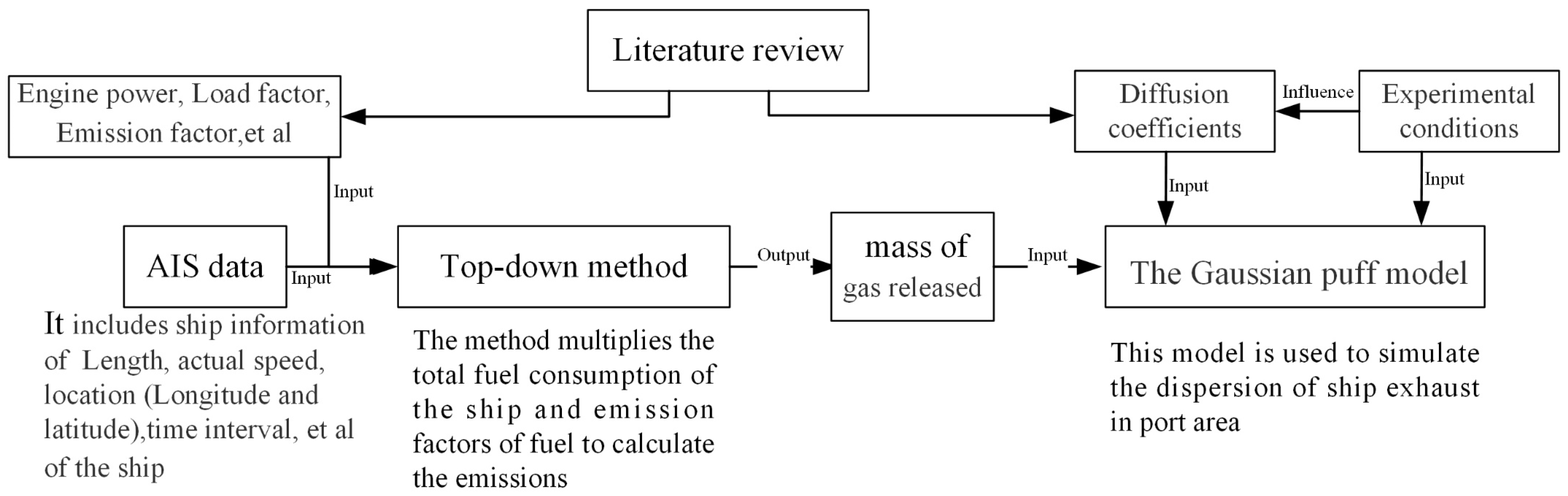
2. Methodology
2.1. Mathematical Model
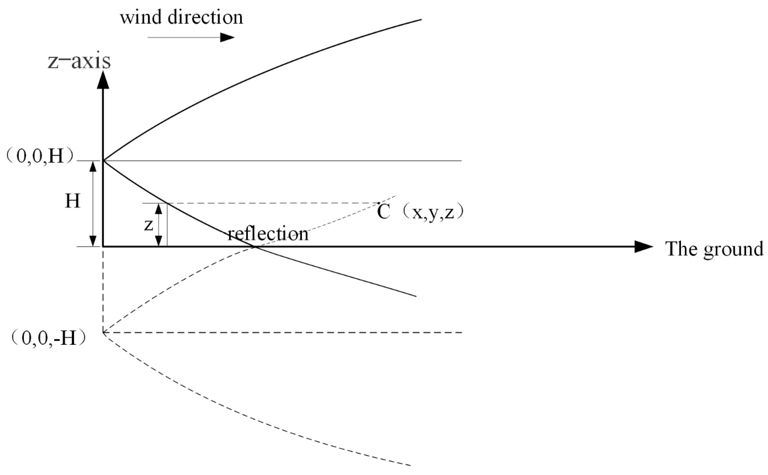
2.1.1. Diffusion Model
2.1.2. Calculation Model of Exhaust Gas
2.2. Model Parameters
2.2.1. Parameters of Diffusion Model
2.2.2. Parameters of Emission Calculation
- (1)
- Engine powerThe engine power of a ship is important datum for calculating ship emissions. However, accurate ship power data are often not disclosed, making it difficult to obtain them. When calculating ship emissions, this study refers to ship information published by the China Classification Society (CCS) and relevant research, divides the ships in port waters into inland ships, coastal ships, and ocean ships, and determines the calculation method of engine power as described in the following sections.
- 1)
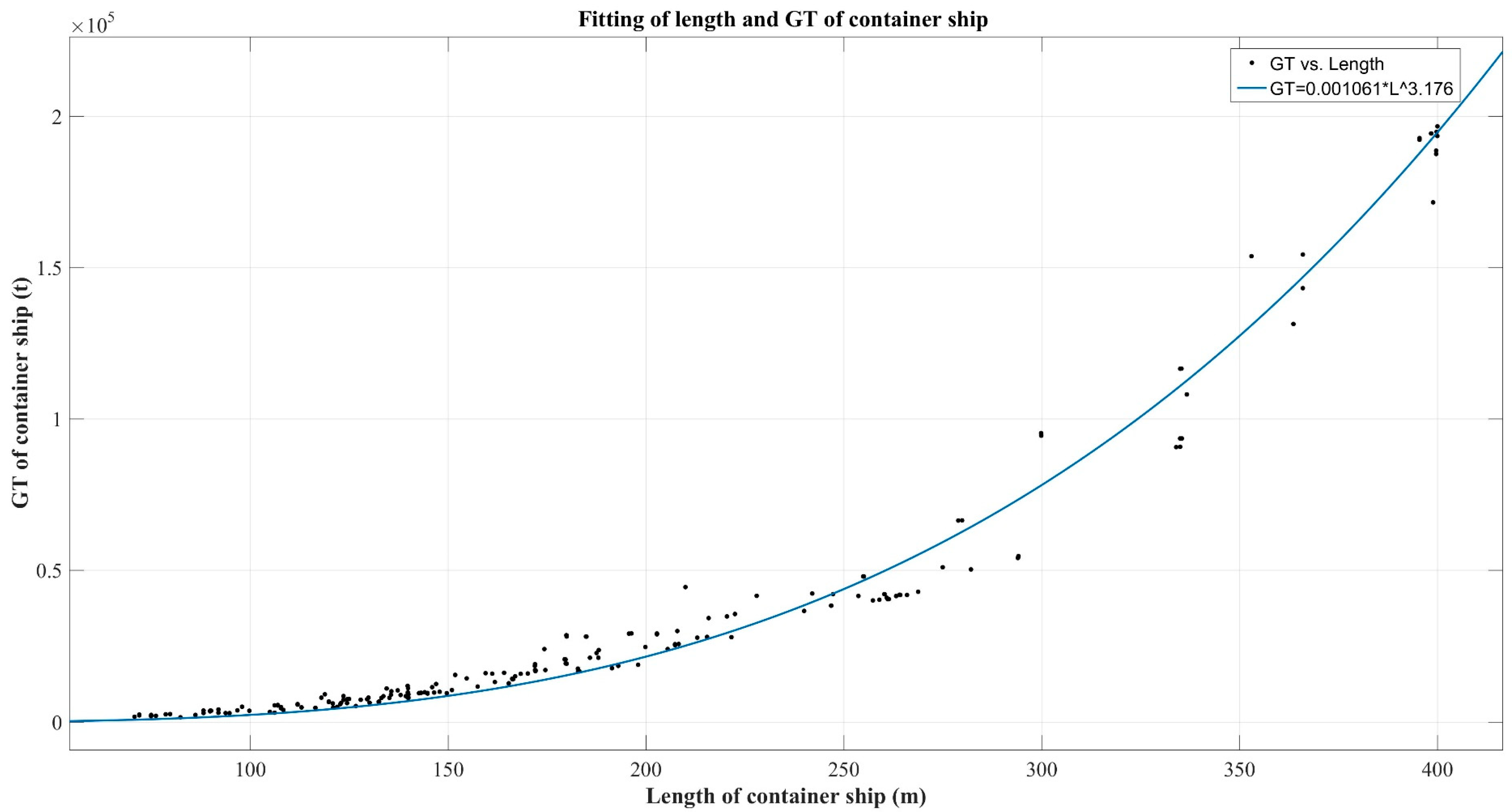
- Main engine powerThis paper selects a fitting formula based on the gross tonnage and main engine power to estimate the ship power of the main engine. The gross tonnage (GT) is estimated by the ship’s length. The method [32] is presented in Table 4 and Table 5.To estimate the power of container ships, this study assumes that hull structures of container ships are highly similar (container ships are loaded with standard containers). Therefore, this study determines the power of container ships using fitting data published by the CCS.A total of more than 600 container ships were selected for this study; we fit the relationship between the length and the GT of the ship, calculating the quantity relationship as follows:where x is the length of ship and y is GT. Figure 3 shows the fitting results.Based on the relationship between the length and GT, the fitted formula in the study [33] is selected to measure the relationship between GT and main engine power of the container ship:The engine power of the fishing ship is calculated using the Statistical Yearbook of Guangdong Province. In 2020, there were 2115 fishing ships in Shenzhen, with a total power of 110,728 kW. It is difficult to complete a detailed division of the types and operation modes; as such, this study uses the average value of 110,728/2115 =52.4 kW as the main engine power of an average fishing ship in Shenzhen Port.
- 2)
- Auxiliary engine power
Due to the shortage of information about the rated power of the auxiliary engine, the AE-rated power of a specific ship type is estimated by using the power ratio of AE to ME according to past experience with emission inventories. Based on [33], the power ratios used in this study are presented in Table 6.
- (2)
- Running state of the ship’s main engine
- (3)
- Load factor
- (4)
- Emission factor
3. Case Study
3.1. Simulation Experiment Design
3.1.1. Assumptions
- (1)
- The atmospheric stability, wind speed, wind direction, and other meteorological conditions are stable during the study period;
- (2)
- The theoretical premise of the Gaussian diffusion model is valid;
- (3)
- Assume that the sea level and land are at the same level;
- (4)
- The ship track is segmented based on the reported interval in AIS, and the emission generated in each segment is considered to be a puff;
- (5)
- AIS data are normal data and errors are not considered.
3.1.2. Representative Pollutant and Damage
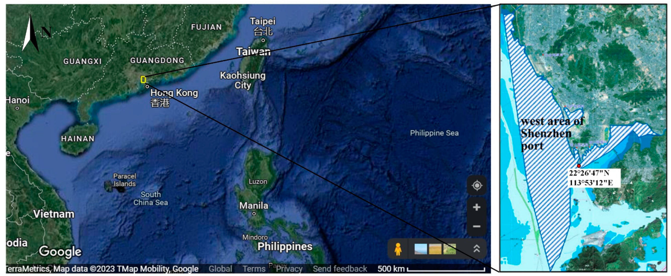
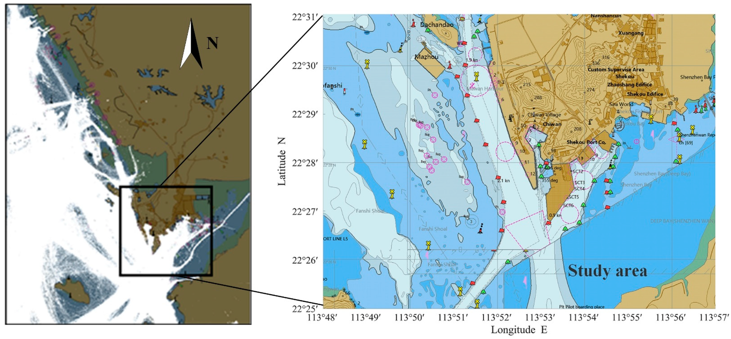
3.1.3. Experimental Area
3.1.4. Effective Source Height
3.1.5. Meteorological Conditions
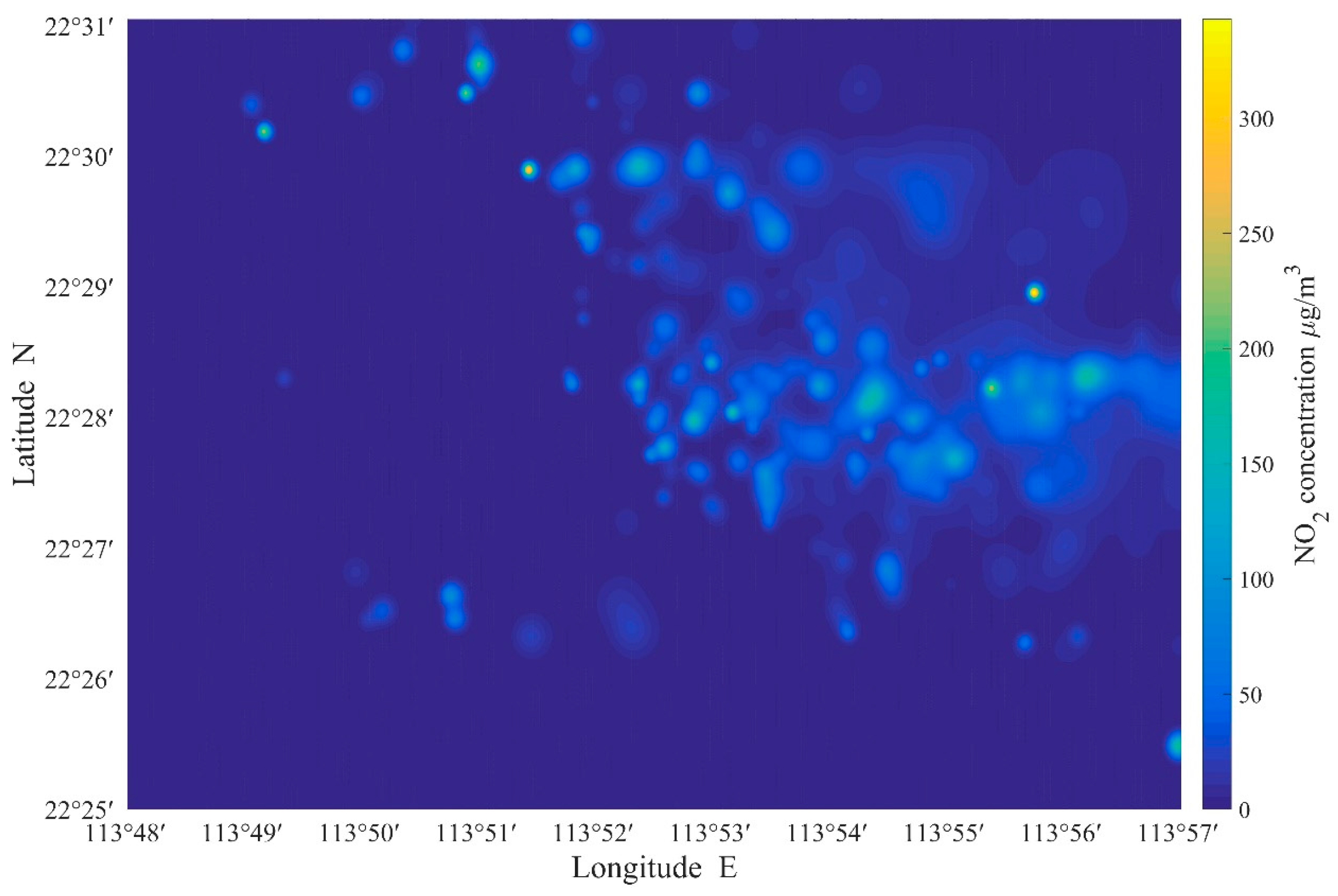
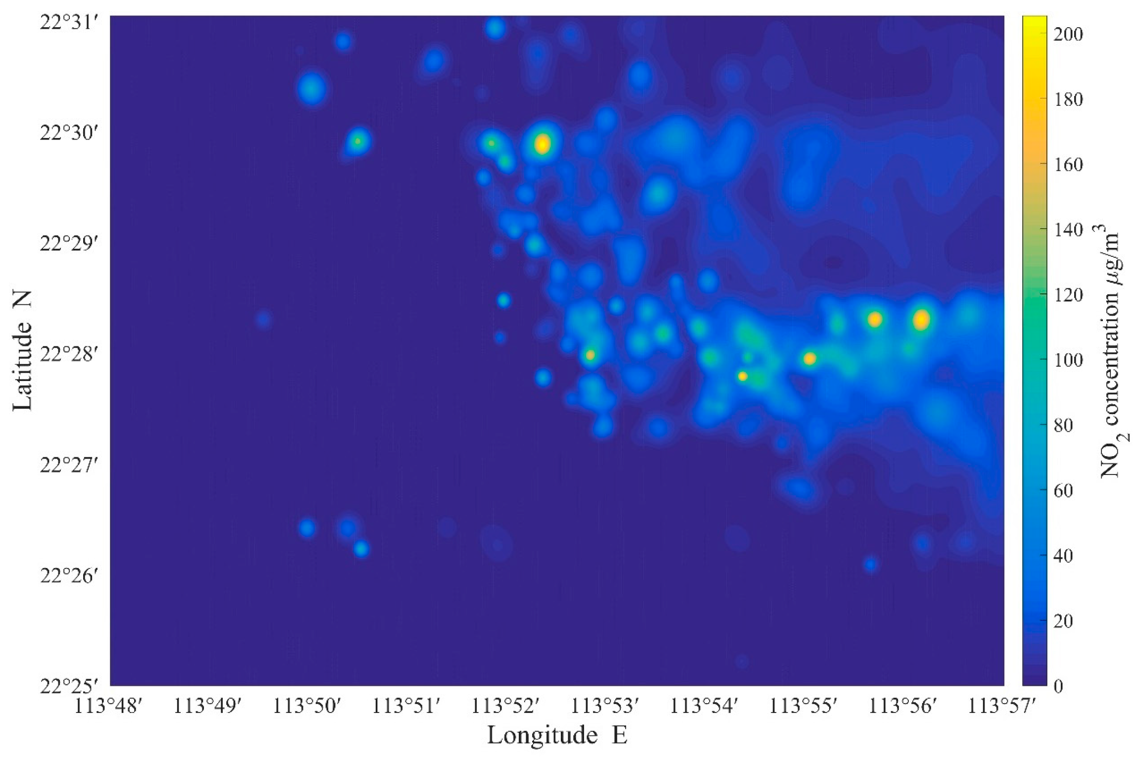
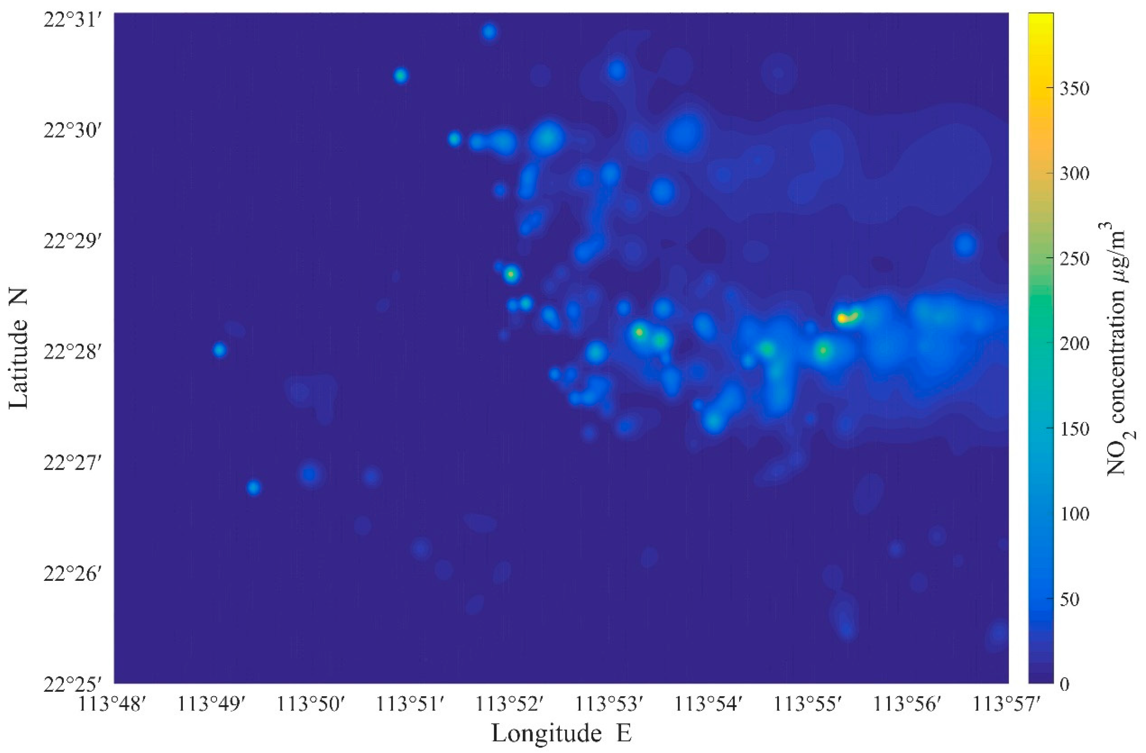
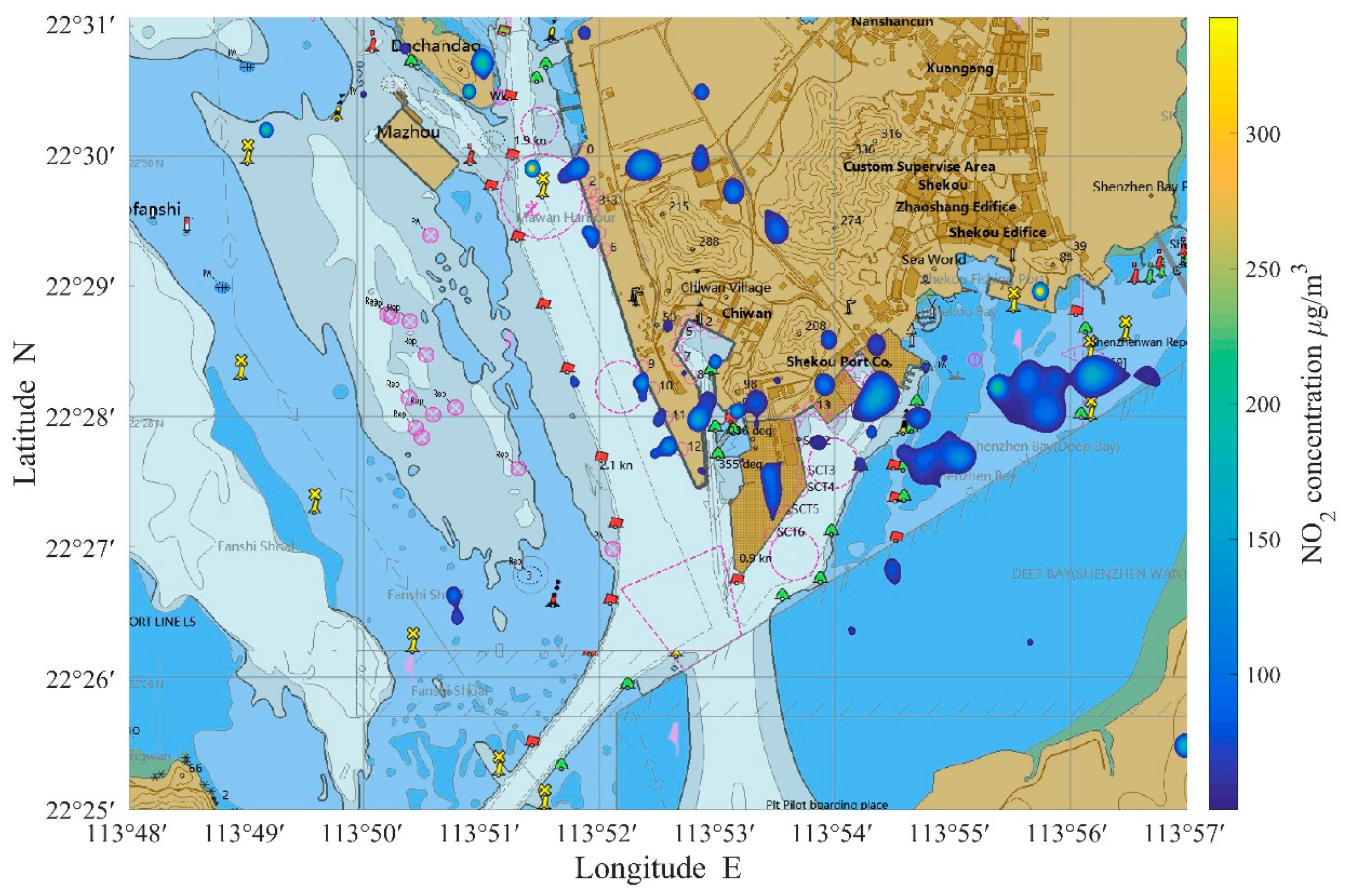
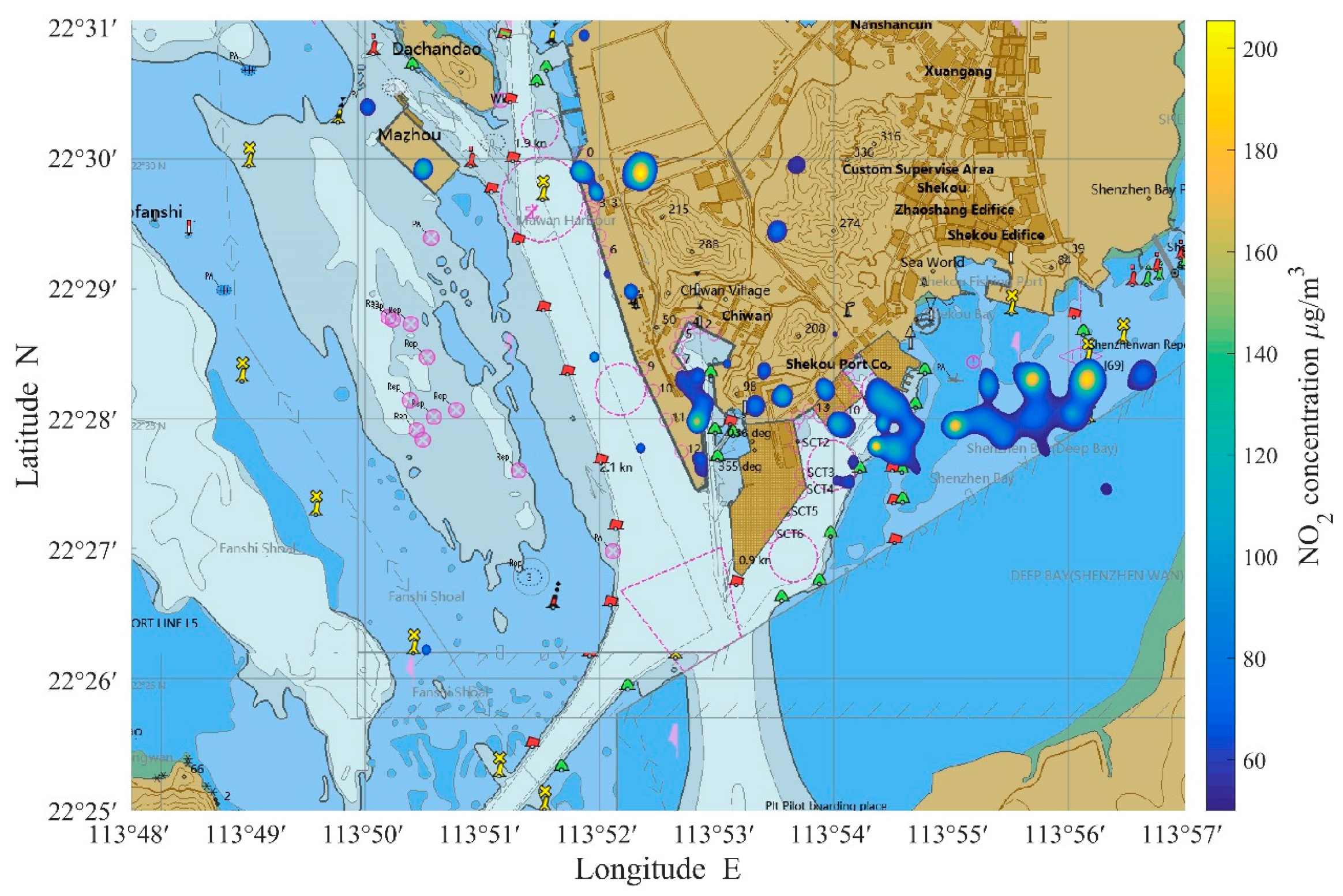
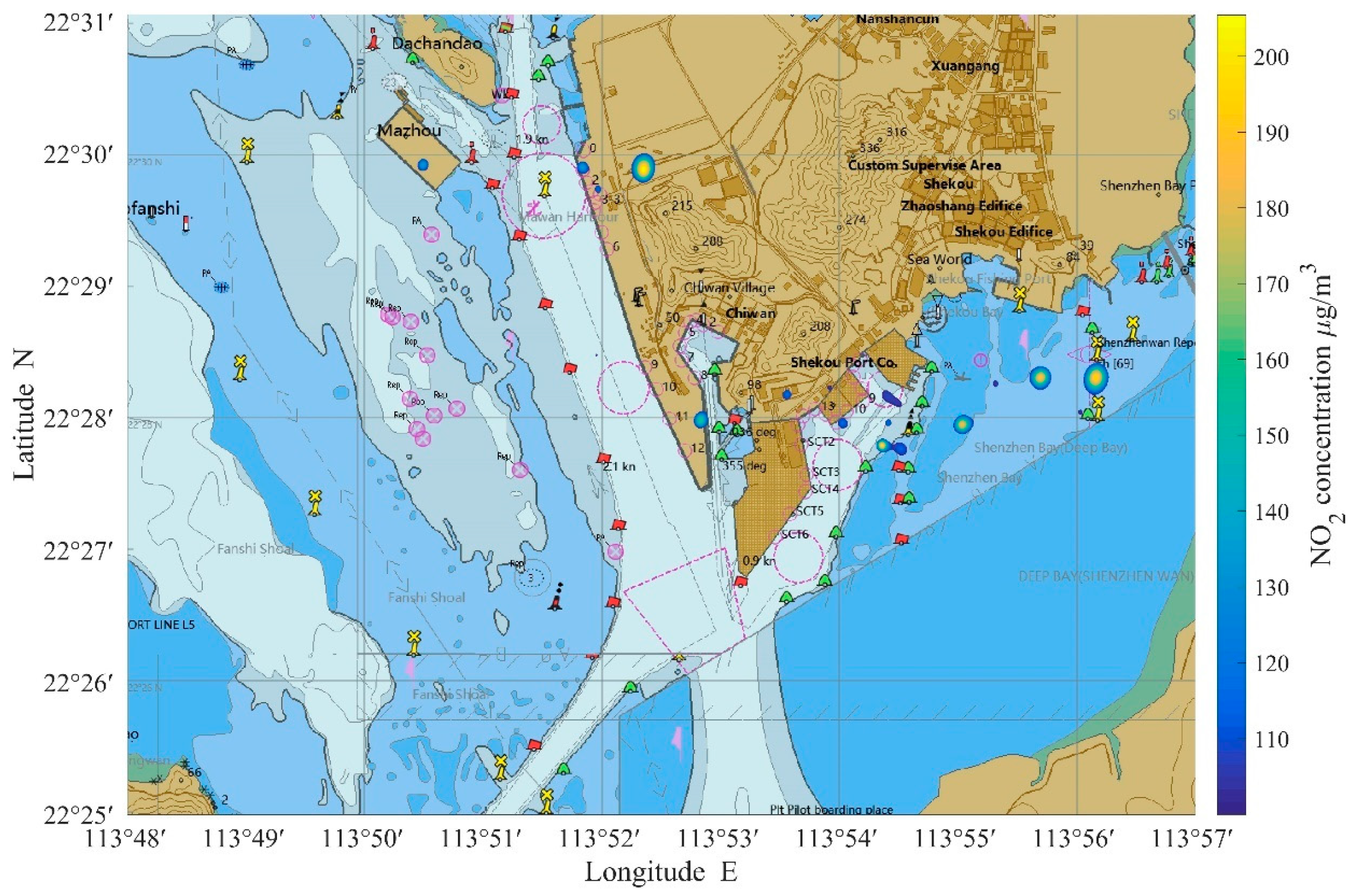
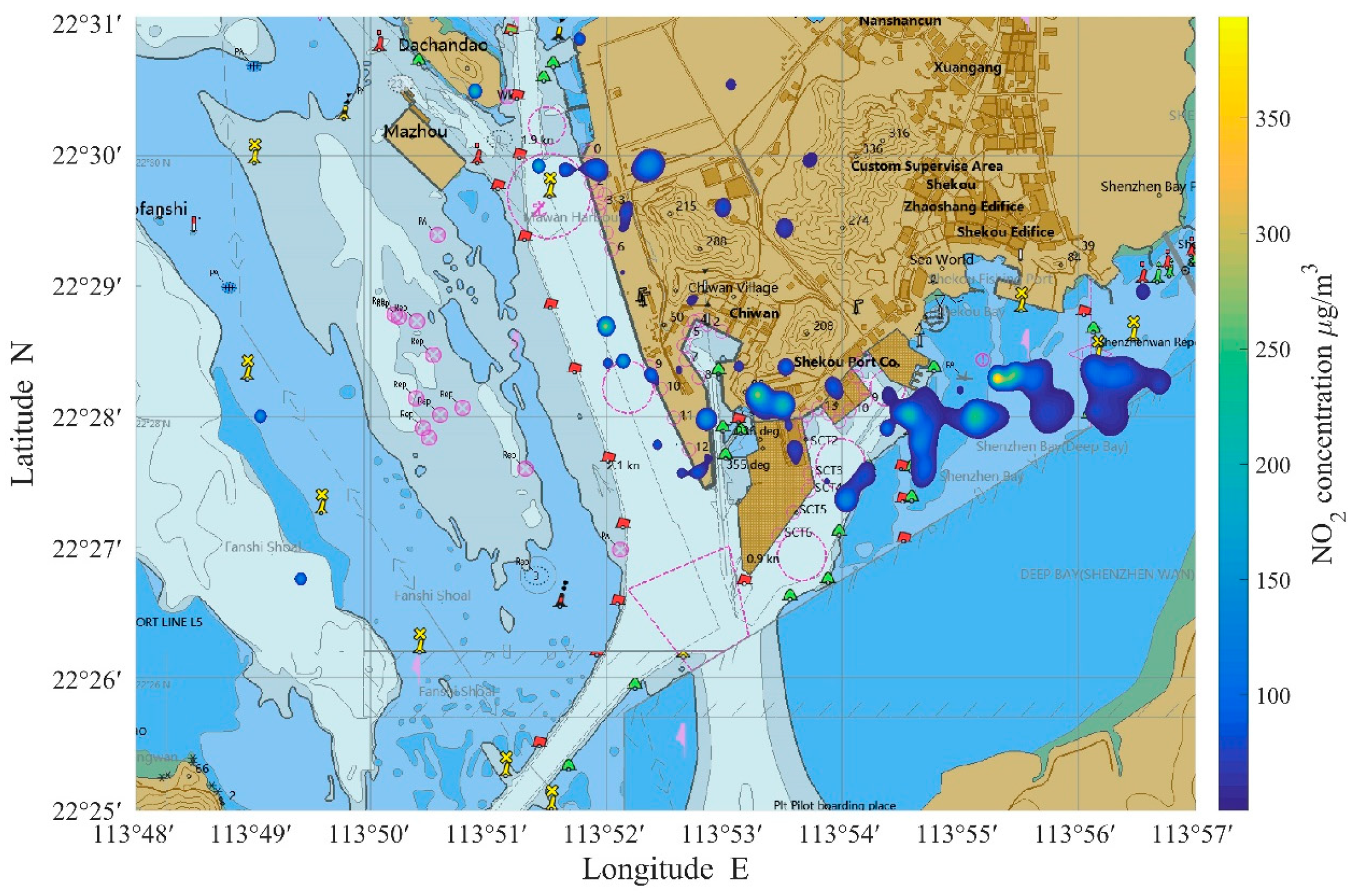
3.2. Results
4. Discussion
5. Conclusions
Author Contributions
Funding
Institutional Review Board Statement
Informed Consent Statement
Data Availability Statement
Conflicts of Interest
Appendix A

| Load | SO2 | NOx | PM | HC | CO |
|---|---|---|---|---|---|
| 1.00% | 1 | 11.47 | 19.17 | 59.28 | 19.32 |
| 2.00% | 1 | 4.63 | 7.29 | 21.18 | 9.68 |
| 3.00% | 1 | 2.92 | 4.33 | 11.68 | 6.46 |
| 4.00% | 1 | 2.21 | 3.09 | 7.71 | 4.86 |
| 5.00% | 1 | 1.83 | 2.44 | 5.61 | 3.89 |
| 6.00% | 1 | 1.6 | 2.04 | 4.35 | 3.25 |
| 7.00% | 1 | 1.45 | 1.79 | 3.52 | 2.79 |
| 8.00% | 1 | 1.35 | 1.61 | 2.95 | 2.45 |
| 9.00% | 1 | 1.27 | 1.48 | 2.52 | 2.18 |
| 10.00% | 1 | 1.22 | 1.38 | 2.18 | 1.96 |
| 11.00% | 1 | 1.17 | 1.3 | 1.96 | 1.79 |
| 12.00% | 1 | 1.14 | 1.24 | 1.76 | 1.64 |
| 13.00% | 1 | 1.11 | 1.19 | 1.6 | 1.52 |
| 14.00% | 1 | 1.08 | 1.15 | 1.47 | 1.41 |
| 15.00% | 1 | 1.06 | 1.11 | 1.36 | 1.32 |
| 16.00% | 1 | 1.05 | 1.08 | 1.26 | 1.24 |
| 17.00% | 1 | 1.03 | 1.06 | 1.18 | 1.17 |
| 18.00% | 1 | 1.02 | 1.04 | 1.11 | 1.11 |
| 19.00% | 1 | 1.01 | 1.02 | 1.05 | 1.05 |
| 20.00% | 1 | 1 | 1 | 1 | 1 |
| Engine Type | Fuel Type | Sulfur Content | Pollutant | ||||||
|---|---|---|---|---|---|---|---|---|---|
| SO2 | NOx | PM10 | PM2.5 1) | HC 2) | CO | ||||
| Ocean ship/Coastal ship | Medium speed (ME) | HFO | 2.70% | 10.29 | 18.10 | 1.42 | 1.31 | 0.60 | 1.40 |
| MDO | 1.00% | 3.62 | 17.00 | 0.45 | 0.42 | 0.60 | 1.40 | ||
| MGO | 0.50% | 1.81 | 17.00 | 0.31 | 0.28 | 0.60 | 1.40 | ||
| Low speed (ME) | HFO | 2.70% | 11.24 | 14.00 | 1.43 | 1.32 | 0.50 | 1.10 | |
| MDO | 1.00% | 3.97 | 13.20 | 0.47 | 0.43 | 0.50 | 1.10 | ||
| MGO | 0.50% | 1.98 | 13.20 | 0.31 | 0.29 | 0.50 | 1.10 | ||
| AE | HFO | 2.70% | 11.98 | 14.70 | 1.44 | 1.32 | 0.40 | 1.10 | |
| MDO | 1.00% | 4.24 | 13.90 | 0.49 | 0.45 | 0.40 | 1.10 | ||
| MGO | 0.50% | 2.12 | 13.90 | 0.32 | 0.29 | 0.40 | 1.10 | ||
| Inland ship | ME 3) | MGO | 0.50% | 2.08 | 10.00 | 0.30 | 0.29 | 0.27 | 1.50 |
| ME 4) | MGO | 0.50% | 2.08 | 13.20 | 0.72 | 0.70 | 0.50 | 1.10 | |
| ME 5) | MGO | 0.50% | 2.08 | 13.20 | 0.31 | 0.29 | 0.47 | 1.10 | |
| AE 6) | MGO | 0.50% | 2.08 | 10.00 | 0.40 | 0.39 | 0.27 | 1.70 | |
| AE 5) | MGO | 0.50% | 2.12 | 10.00 | 0.31 | 0.29 | 0.26 | 1.50 | |
| Type | SO2 | NOx | CO | PM10 1) | HC 2) |
|---|---|---|---|---|---|
| Inland ship | 30.0 | 46.3 | 8.8 | 2.4 | 4.6 |
| Coastal ship | 30.0 | 60.1 | 7.0 | 2.4 | 3.2 |
| Average | 30.0 | 53.2 | 7.9 | 2.4 | 3.9 |
References
- UNCTAD. Review of Maritime Transport 2017. 2017. Available online: https://unctad.org/system/files/official-document/rmt2017_en.pdf (accessed on 10 December 2022).
- Song, S. Ship emissions inventory, social cost and eco-efficiency in Shanghai Yangshan port. Atmos. Environ. 2014, 82, 288–297. [Google Scholar] [CrossRef]
- Sampson, H.; Bloor, M.; Baker, S.; Dahlgren, K. Greener shipping? A consideration of the issues associated with the introduction of emission control areas. Marit. Policy Manag. 2016, 43, 295–308. [Google Scholar] [CrossRef]
- Ma, W.; Lu, T.; Ma, D.; Wang, D.; Qu, F. Ship route and speed multi-objective optimization considering weather conditions and emission control area regulations. Marit. Policy Manag. 2021, 48, 1053–1068. [Google Scholar] [CrossRef]
- Ma, W.; Hao, S.; Ma, D.; Wang, D.; Jin, S.; Qu, F. Scheduling decision model of liner shipping considering emission control areas regulations. Appl. Ocean. Res. 2021, 106, 102416. [Google Scholar] [CrossRef]
- Ma, D.; Ma, W.; Jin, S.; Ma, X. Method for simultaneously optimizing ship route and speed with emission control areas. Ocean. Eng. 2020, 202, 107170. [Google Scholar] [CrossRef]
- Collins, B.; Sanderson, M.G.; Johnson, C.E. Impact of increasing ship emissions on air quality and deposition over Europe by 2030. Meteorol. Z. 2009, 18, 25. [Google Scholar] [CrossRef] [PubMed]
- Liu, H.; Fu, M.; Jin, X.; Shang, Y.; Shindell, D.; Faluvegi, G.; Shindell, K.; He, K. Health and climate impacts of ocean-going vessels in East Asia. Nat. Clim. Change 2016, 6, 1037–1041. [Google Scholar] [CrossRef]
- Song, S.K.; Shon, Z.H. Current and future emission estimates of exhaust gases and particles from shipping at the largest port in Korea. Environ. Sci. Pollut. Res. 2014, 21, 6612–6622. [Google Scholar] [CrossRef]
- Corbett, J.J.; Fischbeck, P.S.; Pandis, S.N. Global nitrogen and sulfur inventories for oceangoing ships. J. Geophys. Res. Atmos. 1999, 104, 3457–3470. [Google Scholar] [CrossRef]
- Endresen, Ø.; Sørgård, E.; Behrens, H.L.; Brett, P.O.; Isaksen, I.S. A historical reconstruction of ships’ fuel consumption and emissions. J. Geophys. Res. Atmos. 2007, 112. [Google Scholar] [CrossRef] [Green Version]
- Jalkanen, J.P.; Johansson, L.; Kukkonen, J.; Brink, A.; Kalli, J.; Stipa, T. Extension of an assessment model of ship traffic exhaust emissions for particulate matter and carbon monoxide. Atmos. Chem. Phys. 2012, 12, 2641–2659. [Google Scholar] [CrossRef]
- Ng, S.K.; Loh, C.; Lin, C.; Booth, V.; Chan, J.W.; Yip, A.C.; Li, Y.; Lau, A.K. Policy change driven by an AIS-assisted marine emission inventory in Hong Kong and the Pearl River Delta. Atmos. Environ. 2013, 76, 102–112. [Google Scholar] [CrossRef]
- Jalkanen, J.P.; Johansson, L.; Kukkonen, J. A comprehensive inventory of the ship traffic exhaust emissions in the Baltic Sea from 2006 to 2009. Ambio 2014, 43, 311–324. [Google Scholar] [CrossRef] [PubMed]
- Xing, H.; Duan, S.L.; Liang, B.N.; Liu, Q.A. Methods to estimate exhaust emissions from sea-going ships according to operational data. Navig. China 2016, 39, 93–98. [Google Scholar]
- Jalkanen, J.P.; Brink, A.; Kalli, J.; Pettersson, H.; Kukkonen, J.; Stipa, T. A modelling system for the exhaust emissions of marine traffic and its application in the Baltic Sea area. Atmos. Chem. Phys. 2009, 9, 9209–9223. [Google Scholar] [CrossRef]
- Fan, Q.; Zhang, Y.; Ma, W.; Ma, H.; Feng, J.; Yu, Q.; Yang, X.; Chen, L. Spatial and seasonal dynamics of ship emissions over the Yangtze River Delta and East China Sea and their potential environmental influence. Environ. Sci. Technol. 2016, 50, 1322–1329. [Google Scholar] [CrossRef]
- Wan, Z.; Ji, S.; Liu, Y.; Zhang, Q.; Chen, J.; Wang, Q. Shipping emission inventories in China’s Bohai Bay, Yangtze River Delta, and Pearl River Delta in 2018. Mar. Pollut. Bull. 2020, 151, 110882. [Google Scholar] [CrossRef]
- He, S.; Wu, X.; Wang, J.; Guo, J. A ship emission diffusion model based on translation calculation and its application on Huangpu River in Shanghai. Comput. Ind. Eng. 2022, 172, 108569. [Google Scholar] [CrossRef]
- Nagendra, S.; Khare, M.; Gulia, S.; Vijay, P.; Chithra, V.S.; Bell, M.; Namdeo, A. Application of ADMS and AERMOD models to study the dispersion of vehicular pollutants in urban areas of India and the United Kingdom. WIT Trans. Ecol. Environ. 2012, 157, 3–12. [Google Scholar]
- Byun, D.; Schere, K.L. Review of the governing equations, computational algorithms, and other components of the Models-3 Community Multiscale Air Quality (CMAQ) modeling system. Appl. Mech. Rev. 2006, 59, 51–77. [Google Scholar] [CrossRef]
- Ariana, M.; Pitana, T.; Artana, K.B.; Dinariyana, B.; Masroeri, A.A. Gaussian plume and puff model to estimate ship emission dispersion by combining automatic identification system (AIS) and geographic information system (GIS). J. Marit. Res. 2013, 3, 1–13. [Google Scholar]
- Bai, S.; Wen, Y.; He, L.; Liu, Y.; Zhang, Y.; Yu, Q.; Ma, W. Single-vessel plume dispersion simulation: Method and a case study using CALPUFF in the Yantian port area, Shenzhen (China). Int. J. Environ. Res. Public Health 2020, 17, 7831. [Google Scholar] [CrossRef] [PubMed]
- Murena, F.; Mocerino, L.; Quaranta, F.; Toscano, D. Impact on air quality of cruise ship emissions in Naples, Italy. Atmos. Environ. 2018, 187, 70–83. [Google Scholar] [CrossRef]
- Peng, X.; Wen, Y.; Xiao, C.; Huang, L.; Zhou, C.; Zhang, F.; Zhang, Y. Improved calculation model for ship exhaust emission dispersion. J. Saf. Environ. 2020, 20, 255–264. Available online: https://zhikuyun.xinhua.org/Liems/web/result/detail.htm?index=cgk_journal&type=achievement&id=CJFDAUTO_AQHJ202001034 (accessed on 10 December 2022).
- Sausen, R. Transport impacts on atmosphere and climate: The ATTICA assessment report. Atmos. Environ. 2010, 44, 4645–4816. [Google Scholar] [CrossRef]
- Matthias, V.; Bewersdorff, I.; Aulinger, A.; Quante, M. The contribution of ship emissions to air pollution in the North Sea regions. Environ. Pollut. 2010, 158, 2241–2250. [Google Scholar] [CrossRef]
- Sharan, M.; Yadav, A.K.; Singh, M.P. Plume dispersion simulation in low-wind conditions using coupled plume segment and Gaussian puff approaches. J. Appl. Meteorol. Climatol. 1996, 35, 1625–1631. [Google Scholar] [CrossRef]
- Li, K.; Liang, M.; Su, G. Data assimilation method for atmospheric dispersion based on a Gaussian puff model. J. Tsinghua Univ. (Sci. Technol.) 2018, 58, 992–999. [Google Scholar]
- Liu, Y.; Lu, W.; Wang, H.; Huang, Q.; Gao, X. Odor impact assessment of trace sulfur compounds from working faces of landfills in Beijing, China. J. Environ. Manag. 2018, 220, 136–141. [Google Scholar] [CrossRef]
- Herrería-Alonso, S.; Suárez-González, A.; Rodríguez-Pérez, M.; Rodríguez-Rubio, R.F.; López-García, C. A solar altitude angle model for efficient solar energy predictions. Sensors 2020, 20, 1391. [Google Scholar] [CrossRef]
- Zhu, Q.; Liao, C.; Wang, L.; Han, H.; Liu, J.; Zhang, Y.; Zeng, W. Application of fine vessel emission inventory compilation method based on AIS data. China Environ. Sci. 2017, 37, 4493–4500. [Google Scholar]
- Chen, D.; Wang, X.; Li, Y.; Lang, J.; Zhou, Y.; Guo, X.; Zhao, Y. High-spatiotemporal-resolution ship emission inventory of China based on AIS data in 2014. Sci. Total Environ. 2017, 609, 776–787. [Google Scholar] [CrossRef] [PubMed]
- Ng SK, W.; Lin, C.; Chan, J.W.M. Study on marine vessels emission inventory, final report. Hong Kong China Hong Kong Environ. Prot. Dep. 2012, 2012, 9–103. [Google Scholar]
- Yang, J.; Yin, P.L.; Si-Qi, Y.; Wang, S.S.; Zheng, J.Y.; Ou, J.M. Marine emission inventory and its temporal and spatial characteristics in the city of Shenzhen. Environ. Sci. 2015, 36, 1217–1226. [Google Scholar]
- Guo, H.; Gu, X.; Ma, G.; Shi, S.; Wang, W.; Zuo, X.; Zhang, X. Spatial and temporal variations of air quality and six air pollutants in China during 2015–2017. Sci. Rep. 2019, 9, 15201. [Google Scholar] [CrossRef]
- Gan, L.; Che, W.; Zhou, M.; Zhou, C.; Zheng, Y.; Zhang, L.; Rangel-Buitrago, N.; Song, L. Ship exhaust emission estimation and analysis using Automatic Identification System data: The west area of Shenzhen port, China, as a case study. Ocean. Coast. Manag. 2022, 226, 106245. [Google Scholar] [CrossRef]
- Sun, W.Y.; Ding, S.L.; Zeng, S.S.; Su, S.J.; Jiang, W.J. Simultaneous absorption of NOx and SO2 from flue gas with pyrolusite slurry combined with gas-phase oxidation of NO using ozone. J. Hazard. Mater. 2011, 192, 124–130. [Google Scholar] [CrossRef]
- Mocerino, L.; Murena, F.; Quaranta, F.; Toscano, D. A methodology for the design of an effective air quality monitoring network in port areas. Sci. Rep. 2020, 10, 1–10. [Google Scholar] [CrossRef] [PubMed] [Green Version]
- Chen, Q.; Lau, Y.Y.; Ge, Y.E.; Dulebenets, M.A.; Kawasaki, T.; Ng, A.K. Interactions between Arctic passenger ship activities and emissions. Transp. Res. Part D Transp. Environ. 2021, 97, 102925. [Google Scholar] [CrossRef]
- Shu, Y.; Wang, X.; Huang, Z.; Song, L.; Fei, Z.; Gan, L.; Xu, Y.; Yin, J. Estimating spatiotemporal distribution of wastewater generated by ships in coastal areas. Ocean. Coast. Manag. 2022, 222, 106133. [Google Scholar] [CrossRef]
- Kesgin, U.; Vardar, N. A study on exhaust gas emissions from ships in Turkish Straits. Atmos. Environ. 2001, 35, 1863–1870. [Google Scholar] [CrossRef]


| Atmospheric Stability | ||
|---|---|---|
| A | 0.2d | |
| B | 0.12d | |
| C | ||
| D | ||
| E | ||
| F |
| Ground Wind Speed m/s | Intensity of Solar Radiation | |||||
|---|---|---|---|---|---|---|
| +3 | +2 | +1 | 0 | −1 | −2 | |
| ≤1.9 | A | A–B | B | D | E | F |
| 2–2.9 | A–B | B | C | D | E | F |
| 3–4.9 | B | B–C | C | D | D | E |
| 5–5.9 | C | C–D | D | D | D | D |
| 6 | D | D | D | D | D | D |
| Total Cloud Cover/Low Cloud Cover | At Night | Solar Altitude h | |||
| 4/4 | −2 | −1 | +1 | +2 | +3 |
| 5–7/4 | −1 | 0 | +1 | +2 | +3 |
| 8/4 | −1 | 0 | 0 | +1 | +1 |
| 7/5–7 | 0 | 0 | 0 | 0 | +1 |
| 8/8 | 0 | 0 | 0 | 0 | 0 |
| Ship Type | Relationship | |
|---|---|---|
| Ocean ship | Cargo ship | |
| Tanker | ||
| Tug | ||
| Other | ||
| Coastal ship | Cargo ship | |
| Tanker | ||
| Tug | ||
| Other | ||
| Inland ship | Cargo ship | |
| Tanker | ||
| Tug | ||
| Other | ||
| Passenger ship |
| Ship Type | Relation | |
|---|---|---|
| Ocean ship | Cargo ship | |
| Tanker | ||
| Tug | ||
| Other | ||
| Coastal ship | Cargo ship | |
| Tanker | ||
| Tug | ||
| Other | ||
| Inland ship | Cargo ship | |
| Tanker | ||
| Tug | ||
| Other | ||
| Passenger ship | 200 kw (GT ≤ 200 t) 250 kw (GT ≤ 400 t) 510 kw (GT > 400 t) |
| Ship Type | Auxiliary Engine/Main Engine |
|---|---|
| Tanker | 0.211 |
| Cargo ship | 0.220 |
| Container ship | 0.220 |
| Tug | 0.221 |
| Passenger ship | 0.278 |
| Fishing ship | 0.222 |
| Other | 0.222 |
| Scheme | Normal Cruising | Slow-Steaming | Accessing Berth/Anchorage | Anchoring or Berthing |
|---|---|---|---|---|
| Speed limit | v > 11 kn | 11 kn ≥ v ≥ 6 kn | 1 kn < v ≤ 6 kn | v ≤ 1 kn |
| Ship Type | Maximum Speed (kn) | |
|---|---|---|
| Ocean ship | Container ship | 21 |
| Tanker | 16 1) | |
| Cargo ship | 16 | |
| Passenger ship | 22 | |
| Other | 14.2 | |
| Coastal ship | Container ship | 15 |
| Tanker | 13 | |
| Cargo ship | 14 | |
| High-speed passenger ship | 42 | |
| Other | 11.5 | |
| Inland ship | Container ship | 11 |
| Tanker | 11 | |
| Cargo ship | 12 | |
| Passenger ship | 8.2 | |
| Other | 9.3 |
| Air Quality Index | Air Quality Level | Health Impact on Residents |
|---|---|---|
| 0–50 | Excellent | Essentially no air pollution |
| 51–100 | Good | Some pollutants may have a weak impact on the health of a few highly sensitive people |
| 101–150 | Slight pollution | Symptoms of susceptible people are slightly aggravated, healthy people experience discomfort |
| 151–200 | Moderate pollution | May further aggravate the symptoms of susceptible people, may affect the heart and respiratory system of healthy people |
| 201–300 | Heavy pollution | Symptoms of patients with heart disease and lung disease are significantly aggravated, exercise tolerance is reduced, symptoms are common among healthy people |
| >300 | Serious pollution | Healthy people have strong symptoms, and some diseases appear earlier than normal |
| Individual Air Quality Index | Concentration Limit of Pollutant | |||||||
|---|---|---|---|---|---|---|---|---|
| SO2 24 h Average/ (μg/m3) | SO2 1 h Average/ (μg/m3) | NO2 24 h Average/ (μg/m3) | NO2 1 h Average/ (μg/m3) | PM10 24 h Average/ (μg/m3) | CO 24 h Average/ (μg/m3) | CO 1 h Average/ (μg/m3) | PM2.5 24 h Average/ (μg/m3) | |
| 0 | 0 | 0 | 0 | 0 | 0 | 0 | 0 | 0 |
| 50 | 50 | 150 | 40 | 100 | 50 | 2 | 5 | 35 |
| 100 | 150 | 500 | 80 | 200 | 150 | 4 | 10 | 75 |
| 150 | 475 | 650 | 180 | 700 | 250 | 14 | 35 | 115 |
| 200 | 800 | 800 | 280 | 1200 | 350 | 24 | 60 | 150 |
| 300 | 1600 | 1) | 565 | 2340 | 420 | 36 | 90 | 250 |
| Length (m) | 100< | 100–200 | 200–300 | >300 |
|---|---|---|---|---|
| Estimated value of chimney height 1) | 12 | 28 | 43 | 50 |
| Atmospheric Stability | A | B | C | D | E | F |
|---|---|---|---|---|---|---|
| Longest distance (m) | About 474 | About 698 | About 1052 | About 1460 | About 2272 | About 3854 |
Disclaimer/Publisher’s Note: The statements, opinions and data contained in all publications are solely those of the individual author(s) and contributor(s) and not of MDPI and/or the editor(s). MDPI and/or the editor(s) disclaim responsibility for any injury to people or property resulting from any ideas, methods, instructions or products referred to in the content. |
© 2023 by the authors. Licensee MDPI, Basel, Switzerland. This article is an open access article distributed under the terms and conditions of the Creative Commons Attribution (CC BY) license (https://creativecommons.org/licenses/by/4.0/).
Share and Cite
Gan, L.; Lu, T.; Shu, Y. Diffusion and Superposition of Ship Exhaust Gas in Port Area Based on Gaussian Puff Model: A Case Study on Shenzhen Port. J. Mar. Sci. Eng. 2023, 11, 330. https://doi.org/10.3390/jmse11020330
Gan L, Lu T, Shu Y. Diffusion and Superposition of Ship Exhaust Gas in Port Area Based on Gaussian Puff Model: A Case Study on Shenzhen Port. Journal of Marine Science and Engineering. 2023; 11(2):330. https://doi.org/10.3390/jmse11020330
Chicago/Turabian StyleGan, Langxiong, Tianfu Lu, and Yaqing Shu. 2023. "Diffusion and Superposition of Ship Exhaust Gas in Port Area Based on Gaussian Puff Model: A Case Study on Shenzhen Port" Journal of Marine Science and Engineering 11, no. 2: 330. https://doi.org/10.3390/jmse11020330