Autonomous Machinery Management for Supervisory Risk Control Using Particle Swarm Optimization

Abstract

Safe navigation for maritime autonomous surface ships (MASS) is a challenging task, and generally highly dependent on effective collaboration between multiple sub-systems in environments with various levels of uncertainty. This paper presents a novel methodology combining risk-based optimal control and path following with autonomous machinery management (AMM) for MASS navigation and supervisory risk control. Specifically, a risk-aware particle swarm optimization (PSO) scheme utilizes “time-to-grounding” predictions based on weather data and electronic navigational charts (ENC) to simultaneously control both the ship’s motion as well as the machinery system operation (MSO) mode during transit. The proposed autonomous navigation system (ANS) is comprised of an online receding horizon control that uses a PSO approach from previous works, which produces a dynamic risk-aware path with respect to grounding obstacles from a pre-planned MASS path, subsequently given as the input to a line-of-sight guidance controller for path following. Moreover, the MSO mode of the AMM system is simultaneously selected and assigned to explicit segments along the risk-aware path throughout the receding horizon, which effectively introduces into the optimization scheme an additional safety layer as well as another dimension for risk or resource minimization. The performance of the resulting ANS is demonstrated and verified through simulations of a challenging scenario and human assessment of the generated paths. The results show that the optimized paths are more efficient and in line with how human navigators would maneuver a ship close to nearby grounding obstacles, compared to the optimized paths of selected previous works.

1. Introduction

An important prerequisite for the realization of autonomous ships is that safe and reliable performance of guidance and navigation tasks is ensured. One possible way of achieving this is to develop risk-based guidance and navigation control systems that uses risk models as part of their decision-making process. Collision avoidance and obstacle avoidance for autonomous guidance and navigation is a topic that recently has received much attention, see for example [1,2,3,4,5,6,7,8,9,10,11,12]. However, reliable obstacle and collision avoidance is not the only concern that should be addressed. Another important aspect of the guidance and navigation task is the grounding risk. Grounding accidents are commonly classified into powered grounding and drifting grounding. Groundings where the ship drifts aground as a consequence of machinery failures are classified as drifting groundings, while groundings that occur due to navigational errors, are referred to as powered groundings [13]. The powered groundings can be seen as part of the obstacle avoidance problem, where the seabed or shore is considered as an obstacle, [14,15,16,17,18,19], while the drifting groundings are not covered by the literature with respect to obstacle avoidance.

Drifting grounding is a problem that, in principle, could be addressed by navigating in such a way as to avoid sailing close to the shore when there is onshore wind. This increases the probability that grounding (following a mechanical or electrical failure) can be prevented by means of dropping anchor or restoring sufficient propulsion and steering capability. There is, however, limited work on autonomous ships where the guidance and navigation problem is studied in terms of drifting grounding avoidance or risk reduction. One study, Blindheim et al. presents a decision-making algorithm to plan suitable trajectories (minimized grounding risk) in situations where the ship unexpectedly experiences reduced maneuverability due to e.g., thruster faults [20]. Moreover, Rokseth and Utne propose a control system for automatically selecting the most appropriate operating mode for a hybrid machinery system in order to minimize the drifting grounding risk and fuel consumption [21].

In this paper, a supervisory control algorithm is proposed, which integrates the machinery system mode selection problem with the guidance and navigation problem, based on data of electronic navigational charts (ENC) from [22]. The main reason why it is of interest to integrate these two control problems is that the controlled states (the ship trajectory and machinery system mode) are important influencing factors for the drifting grounding risk. In general, benefits may be achieved by considering several distinct control problems that share the common feature that they somehow affect the risk associated to the same loss scenario, as this potentially results in an extended or improved set of possible actions for reducing the risk. Thus, the proposed hypothesis is that the potential for reducing the grounding risk at a reasonable operational cost will improve if the two control problems are merged into a single optimization problem weighting both aspects simultaneously, compared to only optimizing for purely spatial and distance-based grounding risks in previous works [23] (see Section 3.5). It is argued that this structure may increase the number of ways in which the control algorithm can make safe decisions, and thus a reasonably safe decision may be computed at a lower operational cost, such as fuel consumption and expected costs based on grounding probabilities.

While the proposed control algorithm in [21] successfully identifies the optimal operating modes, the choice of machinery system operating mode (MSO mode) has a limited impact on both the grounding risk and the fuel consumption. Here, it is instead proposed to model the grounding risk and explicitly address the trade-off between fuel consumption and grounding risk in an optimization framework. A more reliable operational mode is generally more costly in terms of fuel consumption. When the ship is sailing in such a way that the loss of the propulsion power may cause the ship to drift aground in a short amount of time (i.e., close to land while the environmental forces acting on the ship is directed toward the shore), a reliable mode of operation is considerably safer. In this context, a grounding event occurs if the time it takes to drift aground is shorter than the time it takes to recover propulsion capabilities. An alternative way of achieving equal levels of safety is to change the route e.g., such that the ship is sailing further away from grounding obstacles (i.e., the shore or shallow waters) or in such a way that the environmental forces acting on the ship is not directed toward grounding obstacles, or there is more time to recover from a machinery fault.

2. Materials and Methods

2.1. Problem Definition and Approach

In the proposed framework, autonomous ships are following routes defined by a sequence of waypoints (WP). Each waypoint is described with longitude and latitude coordinates. As illustrated in Figure 1, it is assumed that a separate global planning process has prepared a pre-planned route for the entire voyage. This global planning is normally performed onshore when the voyage is planned. Next, a tentative pre-planned route is generated and optimized or adapted online. Thus, the ship re-evaluates the part of the tentative route that falls within a given prediction horizon, while sailing.

The re-planning process consists of two tasks: The first one, referred to as “Level 1 route planning” in Figure 1, is carried out to generate a number of proposed feasible routes. This is achieved by first using the most recent sensor data and map data to check if the part of the tentative route that falls within the prediction horizon passes over objects or too shallow waters that were not identified as obstacles in the planning stage, e.g., if a fish farm has appeared that was not present on the map during voyage planning or the water depth is different due to tides. If not, the tentative route is considered a feasible route. If, on the other hand, there is an obstacle in the way, two alternative routes (one on each side of the obstacle) will be generated (see Appendix A). In principle, $2^N$ options exists if there are N obstacles being considered. It may be noted that this level of re-planning or online avoidance maneuvers may also be applied directly to avoid areas with opposite or dense maritime traffic, nearby vessels or other dynamic obstacles in future works. This could build on preliminary results that combines anti-grounding and anti-collision while considering the traffic rules at sea (COLREGs), albeit without considering MSO and failure modes, as presented in [24].

The second task of the tentative route re-evaluation is to optimize the proposed route alternatives (see “Level 2 route planning” in Figure 1). This is achieved by first generating a new set of intermediate waypoints, essentially increasing the resolution and smoothness of the original tentative route alternative. Next, the new waypoints are adjusted with respect to resource consumption and grounding risk, in which the latitude, longitude and MSO mode for all waypoints of each proposed feasible route are the decision variables available for optimization (Figure 1). Specifically, each adjustment is considered in terms of the total resulting cost, which is a function of the fuel consumption, the grounding risk (using a risk model), and the deviation from the estimated arrival time (ETA) through calculations of the measured states of the sailing process.

The cost related to each proposed control output (adjustment) is estimated through the simulated states from a ship simulator and the probability of grounding from a risk model, and the selected control output of the Level 2 route planner is applied to a sailing process controller—which in turn yields the next measured and/or initial ship states for the subsequent simulation (see the respective modules in Figure 1). Thus, the optimization loop of the Level-2 route planning process is to utilize current measured states from the sailing process as inputs, predict future states using a ship simulator, use these predicted states to estimate grounding risks using a risk model, and weigh these risks against other economic or environmental factors using a cost function to produce an optimized series of waypoints. In this work, an optimization algorithm based on particle swarm optimization (PSO) is used to search for the set of control outputs that results in the lowest overall cost across the receding horizon. PSO was proven to be effective for solving a simplified version of this problem in [23], and was also chosen for solving similar problems related to unmanned aircraft [25,26]. Note that in this proof of concept it is not claimed that PSO is the best method to solve the optimization problem, and it is recommended to study alternative methods such as genetic algorithms in future work.

Figure 2 illustrates the relationship between various factors affecting the cost, as well as the terms that the cost function is composed of. First, the fundamental factors such as ship speed (and available top speed), environmental forces and infrastructure along the shore affects the ETA, grounding risk and fuel consumption as shown in the figure. The position (longitude and latitude) of each waypoint affects the target ETA, i.e., if a WP is moved such that the distance the ship has to sail to reach the target is changed, the ETA and the fuel consumption may change accordingly. Moreover, the grounding risk may change if a waypoint is moved such that the distance between the ship and obstacles is changed, or the duration of exposure to disturbances with respect to e.g., a downwind obstacle changes. Interestingly, the top speed of the ship additionally indirectly affects the ETA. An example may be that longer exposure to increased risks near obstacles of a narrow strait due to a lower available top speed compared to a different ship, can alter the resulting optimal waypoint distribution along a route alternative. The MSO mode (Machinery system config in Figure 2) directly affects the fuel consumption, possible top speed, and additionally the grounding risk because the MSO modes are different in terms of robustness against drifting grounding. Ultimately, the ETA, the grounding risk, and the fuel consumption affect the cost to be minimized.

2.1.1. Level 1 Route Planning

The level 1 planning algorithm from previous works [22] is summarized in Appendix A. It is used to generate pair-wise alternative routes on each side of static grounding obstacles, if any such obstacle crosses the global pre-planned voyage path. Note, however, that the computed paths are only concerned with purely spatial avoidance of any obstacle boundary in the horizontal plane, and is subsequently evaluated, adjusted and optimized with respect to resource consumption and risks by the level 2 route planner.

2.1.2. Level 2 Route Planning

Due to the uncontrolled factors shown in Figure 2, an estimate of expected costs has to be formulated and computed during sailing, based on probabilities and available online (and offline) data. The cost estimate is from Figure 2 given by an ETA, a fuel consumption estimation, and an estimated grounding risk $r_G$, and ultimately serves as the optimization variable for the level 2 route planner. The computation processes for these estimated terms are presented in the following sections.

2.2. Modeling

2.2.1. The Ship Simulator

A three-DOF (degrees of freedom) ship model is proposed, for the purpose of state predictions within the optimization algorithm: The ship’s position ${\mathit{p}}_{b/n}^n$ is described by N (north) and E (east) coordinates, and $\psi$ is the ship’s heading. As seen in (1), its time derivative is a rotation transformation of the ship’s forward (surge) velocity, sideways (sway) velocity and yaw rate are given as u, v and r, respectively. Based on [27], the ship dynamics can be modeled by the notation as presented in

Table 1. An overview of the system variables used in this work.

f	propulsion & steering forces	C	Coriolis matrix	$\delta$	rudder angle
k	proportional coefficient	D	damping matrix	$\mathsf{\eta }$	ship pose
$\mathit{m}$	steering moments	E	easting	$\mathsf{\nu }$	ship velocity
$\mathit{p}$	ship position	F	propulsion force	$\mathsf{\omega }$	rotational velocity
r	yaw rate	$\mathit{J}$	Jacobian matrix	$\psi$	ship heading
u	surge velocity	$\mathit{M}$	mass matrix	$\mathsf{\tau }$	forces & moments
v	sway velocity	N	northing	$\mathsf{\Theta }$	ship orientation
		P	power	$\zeta$	tuning variable
		$\mathit{R}$	rotational matrix

, and the following relationship definitions and equations:

$$\begin{array}{cccccc}\hfill & {\mathit{p}}_{b/n}^n=\left[\begin{array}{c}N\\ E\end{array}\right]\hfill & \hfill & {\mathit{v}}_{b/n}^b=\left[\begin{array}{c}u\\ v\end{array}\right]\hfill & \hfill & {\mathit{R}}_b^n\left({\mathsf{\Theta }}_{nb}\right)=\left[\begin{array}{cc}cos\left(\psi \right)& -sin\left(\psi \right)\\ sin\left(\psi \right)& \phantom{-}cos\left(\psi \right)\end{array}\right]\hfill \\ \hfill & {\mathsf{\Theta }}_{nb}=\left[\begin{array}{c}\psi \end{array}\right]\hfill & \hfill & {\mathsf{\omega }}_{b/n}^b=\left[\begin{array}{c}r\end{array}\right]\hfill \\ \hfill & \mathsf{\eta }=\left[\begin{array}{c}{\mathit{p}}_{b/n}^n\\ {\mathsf{\Theta }}_{nb}\end{array}\right]\hfill & \hfill & \mathsf{\nu }=\left[\begin{array}{c}{\mathit{v}}_{b/n}^b\\ {\mathsf{\omega }}_{b/n}^b\end{array}\right]\hfill & \hfill & {\mathit{J}}_{\mathsf{\Theta }}\left(\mathsf{\eta }\right)=\left[\begin{array}{cc}{\mathit{R}}_b^n\left({\mathsf{\Theta }}_{nb}\right)& \mathbf{0}\\ \mathbf{0}& 1\end{array}\right]\hfill \end{array}$$

$$\begin{array}{cccccc}\hfill & {\dot{\mathit{p}}}_{b/n}^n={\mathit{R}}_b^n\left({\mathsf{\Theta }}_{nb}\right){\mathit{v}}_{b/n}^b\hfill & \hfill & {\dot{\mathsf{\Theta }}}_{nb}={\mathsf{\omega }}_{b/n}^b\hfill & \hfill & \dot{\mathsf{\eta }}={\mathit{J}}_{\mathsf{\Theta }}\left(\mathsf{\eta }\right)\mathsf{\nu }\hfill \end{array}$$

(1)

$$\begin{array}{cccccc}\hfill & {\mathit{f}}_b^b=\left[\begin{array}{c}F\\ -k_{sway}\delta u\end{array}\right]\hfill & \hfill & {\mathit{m}}_b^b=\left[\begin{array}{c}-k_{yaw}\delta u\end{array}\right]\hfill & \hfill & \mathsf{\tau }=\left[\begin{array}{c}{\mathit{f}}_b^b\\ {\mathit{m}}_b^b\end{array}\right]\hfill \end{array}$$

$$\begin{array}{c}\hfill \dot{F}=-\frac{k}{\zeta }F+\frac{1}{\zeta }Pk=\frac{P_{\max }}{F_{\max }}\end{array}$$

(2)

where (2) represents the propulsion force dynamics. Here $\zeta$ is a tuning parameter, F and $F_{\max }$ are the input and maximum propulsion forces, and P and $P_{\max }$ are the input and maximum power available for propulsion, respectively. This model may be found online at GitHub [28].

Equation (3) relates the inertial force given the 3 by 3 mass matrix $\mathit{M}$ (including hydrodynamic added mass) times the acceleration in surge, sway and yaw, with the other forces acting on the vessel. The Coriolis and centripetal forces ${\mathit{C}}_{RB}\left(\mathsf{\nu }\right)\mathsf{\nu }$ and ${\mathit{C}}_A\left({\mathsf{\nu }}_R\right){\mathsf{\nu }}_R$ as described in [29] are included, where ${\nu }_R$ is the ship’s velocity vector relative to a water particle floating with the current, and linear and nonlinear damping terms are described by ${\mathit{D}}_L{\mathsf{\nu }}_R$, and ${\mathit{D}}_{N}L\left({\mathsf{\nu }}_R\right){\mathsf{\nu }}_R$. This gives

$$\mathit{M}\dot{\mathsf{\nu }}=-{\mathit{C}}_{RB}\left(\mathsf{\nu }\right)\mathsf{\nu }-{\mathit{C}}_A\left({\mathsf{\nu }}_R\right){\mathsf{\nu }}_R-{\mathit{D}}_L{\mathsf{\nu }}_R-{\mathit{D}}_{NL}\left({\mathsf{\nu }}_R\right){\mathsf{\nu }}_R+{\mathsf{\tau }}_{wind}+\mathsf{\tau }$$

(3)

where ${\tau }_{wind}$ and $\tau$ represents the wind forces and control forces acting on the ship.

In the presented algorithm, environmental forces are considered as input, and it is not within the scope of this paper to provide algorithms for weather or current forecasting given the terrain and bathymetry. In general, the optimization should include margins when defining the cost function and constraints in order to account for the uncertainty in these forecasts, given the mentioned challenges. In this way, the control system will make robust decisions by taking into account such uncertainty bounds. The example in this work utilizes simple models of the environmental forces which do not include considerations of being close to obstacles or varying depths, for simplicity and clarity when demonstrating the effects of the novel contribution as a proof of concept. The extension to use more complex and accuracy models (if available) is straightforward since the proposed framework is flexible with respect to the format of the provided information (i.e., no requirements have been made for deterministic operations, smoothness or continuity).

2.2.2. The Risk Model

The purpose of the risk model is to estimate the grounding risk $R_G^k$ given in (4) for each simulated future scenario k. In this work, the drifting grounding risk model presented in [21] is defined as follows:

$$R_G^k=P\left(G_k\right)·C_G$$

(4)

It is used as a measure of the grounding risk, where $P\left(G_k\right)$ denotes the probability of experiencing a grounding event $G_k$ during a future prediction horizon in scenario k (if the scenario k were to be executed), and $C_G$ is the cost per grounding.

This model uses ENC data and the position, heading, velocity and yaw rate of a ship as well as nearby grounding obstacles at some time instance t to calculate the probability that a grounding scenario may occur, and can be used as an online real-time risk model for a ship. Note that the grounding obstacles (hazards) are constructed according to [22], in which the desired minimum depth may be selected by the operator. Thus, one may include considerations such as ship size and the water depth in the area around the ship by selecting a minimum depth with an added safety margin.

In this work, the ship’s instantaneous states and relevant map data are fed into the risk model at regular intervals (e.g., every 30 s) to produce an estimate of the probability of grounding in the next time interval, applied repeatedly across a receding horizon of e.g., 1 h to predict future probabilities into an imagined scenario. Thus, the model will be used to evaluate the probability of grounding during a potential future scenario k corresponding to a set of proposed control outputs. In this case, predicted ship states and map data corresponding to scenario k are produced by the ship simulator.

The grounding risk model is illustrated in Figure 3 and deals specifically with the case where the loss of propulsion power may cause the ship to drift aground if propulsion power is not restored in time to prevent it. It is structured as a bow-tie diagram, with unexpected component failures as the triggering events, loss of propulsion power (LOPP) as the hazardous event, and grounding as the considered consequence. This diagram thus conforms with the scope of this paper, i.e., online navigation before a potential loss of propulsion event is considered with respect to grounding risks. Moreover, the MSO modes affect both the engine recovery time during LOPP as well as the potential for unexpected component failures, and may act as proactive barrier if selected appropriately. Lastly, environmental forces (disturbances) and the waypoint positions distributed along the navigated trajectory or path affect the time it would take to ground the ship if a hazardous event occurs.

Figure 4 shows the implementation and structure of the risk model. The hazardous event of Figure 3 serves as the key element in the risk model, in which the probability of a LOPP event occurring is combined with a “time-to-grounding” (TTG) prediction to calculate the accumulating grounding probability distribution across the prediction horizon, based on the future predicted ship states as inputs. This probability is ultimately multiplied with the cost of grounding to produce the total grounding risk $R_G^k$.

2.2.3. The Probability of Grounding

There may be significant transients in $R_G^k$ over the duration of a prediction horizon. To capture the effect of these transients, the prediction horizon is subdivided into n time intervals. $P\left(G_k\right)$ can be formulated as

$$P\left(G_k\right)=\sum _{i=1}^{n}P\left(G_{i,k}\right)$$

(5)

where $G_{i,k}$ denotes the event of grounding during time interval i in scenario k. It is only possible to ground once during the prediction horizon. Therefore, the probability of grounding during a specific interval i in the prediction horizon must account for the possibility that a grounding already occurred earlier in the prediction horizon.

The notation $P\left(G_{i,k}\right|{\overline{G}}_{1,k},{\overline{G}}_{2,k},\dots ,{\overline{G}}_{i-1,k}):=P\left(G_{i,k}\right|{\overline{G}}_{i^{-},k})$ used in (6) is defined as the conditional probability of grounding during the interval i in scenario k, given that it did not occur prior to the i^th interval in scenario k, and ${\overline{G}}_{j,k}$ is the complementary event of $G_{j,k}$. Thus, the probability of grounding during the time interval i in the prediction horizon k can be formulated as

$$\begin{array}{cc}\hfill P\left(G_{i,k}\right)=& \left\{\begin{array}{cc}{\displaystyle P\left(G_{i,k}\right|{\overline{G}}_{i^{-},k})\prod _{j=1}^{i-1}\left(1-P\left(G_{j,k}\right)\right),}\hfill & \mathrm{if}i>1\hfill \\ P\left(G_{1,k}\right),\hfill & \mathrm{if}i=1\hfill \end{array}\right.\hfill \end{array}$$

(6)

Next, each time interval in the prediction horizon k is considered. To simplify the notation, the indices i and k are not included in the following derivation: A potential grounding scenario can be subdivided into a scenario that leads to loss of propulsion power (a LOPP scenario), and a recovery scenario. If a LOPP scenario occurs, a grounding follows if a recovery scenario cannot be successfully executed within the time it takes the ship to drift aground. A LOPP scenario can be described by a set of triggering events, while a recovery scenario is described by a set of startup events. In the model, a set of potential LOPP scenarios is associated to each MSO mode. Moreover, a set of potential recovery scenarios are associated to each LOPP scenario in each MSO mode. That is, the possible ways of recovering the system after LOPP depends on the scenario that caused the LOPP event and the state of the system (MSO mode) when the LOPP event occurred.

Consider the power and propulsion system illustrated in Figure 5 as an example. The system can be operated with two propellers, each with its independent power source. It is assumed that one power source and propeller is sufficient to prevent the ship from grounding. As shown in the fault tree in Figure 6, a potential LOPP scenario, in this case, is that both power sources are lost (i.e., the set containing the two events “ME1 stops” and “ME2 stops”). The event tree in Figure 6 illustrates the two corresponding potential recovery scenarios, namely either the recovery scenario in which ME1 is restarted, or the recovery scenario where ME2 is restarted. If the ship is operated with only one online power source, e.g., ME1, then a LOPP scenario is described by the event “Loss of ME1”, while the potential recovery scenarios becomes “Restart ME1” or “Start ME2”. In general, the event of starting a component and the event of restarting a component are distinguished from each other. Whether one is restarting a component (after unexpected loss) or starting a component may e.g., affect the probability of success.

The probability of experiencing the particular LOPP scenario S consisting of triggering events $e_t$ is denoted $P\left(S\right)$, see (7). If the triggering events can reasonably be modeled as independent events, and the ship is operated in a mode where S is a potential scenario, then

$$P\left(S\right)=\prod _{e_t\in S}P\left(e_t\right).$$

(7)

In this paper, the triggering events $e_t$ are modeled as exponentially distributed events with constant frequencies of occurrence ${\lambda }_t$, as defined in (8). Thus, the probability of experiencing the event $e_t$ during a time interval $\Delta t$ is

$$P\left(e_t\right)=F_{exp}(\Delta t;{\lambda }_t)=1-e^{-{\lambda }_t\Delta t}.$$

(8)

A set $E_r$ of possible recovery scenarios following a particular LOPP scenario in a given machinery system configuration is referred to in a recovery event tree, where each possible recovery scenario $r_i$ is a branch on the event tree (as exemplified in Figure 6). The probability of not succeeding in recovering the system, given the occurrence of LOPP, is equal to the probability that none of the possible recovery scenarios in $E_r$ succeed within the time it takes the ship to drift aground. The probability $P\left(G\right|L)=1-P\left(E_r\right|L)$ of not succeeding in recovering before grounding can be calculated directly from the event tree according to the standard event tree methodology, (e.g., in Figure 6, the probability of grounding given LOPP would be the product of the two probabilities of not restarting ME in time and not restarting M2 in time). To achieve this, it is necessary to find the probability $P\left(e_r\right)$ of each recovery event $e_r$ occurring before grounding (e.g., restarting ME1 in Figure 6). It is noted that the time $\Delta t_r$ it takes from LOPP occurs to event $e_r$ occurs (e.g., M1 is successfully restarted), is a random variable. Thus, the probability that the event occurs before a grounding occurs (i.e., before the time $\Delta t_G$ elapses), is given by the cumulative distribution of $\Delta t_G$, $P(\Delta t_r<\Delta t_G)=F_{e_r}(\Delta t_G)$ and a nominal probability of success $p_r$ associated with the event (e.g., the probability that it is possible to restart ME1 given infinite time),

$$P\left(e_r\right)=F_{e_r}(\Delta t_G)·P\left(r\right).$$

(9)

The time $\Delta t_G$ it would take to ground given the occurrence of LOPP, is found by simulating that the ship drifts without propulsion (and steering), subject to environmental forces. This is achieved by using the TTG simulator for predictions as illustrated in Figure 4. This prediction uses the same model as described in Section 2.2.1, but without propulsion and steering. Lastly, the TTG prediction is initialized by using the predicted ship state each time that LOPP is simulated to occur.

2.2.4. The Cost of Grounding

The cost of grounding is a function of the ship state vector $\mathit{x}$, as illustrated in Figure 4. In general, the cost of grounding can have a large range of contributions. In this research, it is proposed to divide the contributions into costs associated with:

• $C_{ship}:=$ damage to the ship. This depends on the system states $\mathit{x}$, such as impact speed and location of grounding (i.e., the type of surface the ship grounds into), as well as the sea state, $\mathcal{S}$ (i.e., large waves may cause a more violent impact) to be used in the cost function.
• $C_{recovery}:=$ rescue fee that must be paid to recover the ship. This may depend on the constant parameters of the ship such as the length of the ship, but also the system states $\mathit{x}$, and in particular the location of the ship (e.g., if it is far from civilization and the nationality of the rescue team).
• $C_{cargo}:=$ damage to or loss of cargo. This may be set as a fixed parameter according to the value of the cargo, as well as being dependent on the magnitude and nature of the impact.
• $C_{environment}:=$ environmental damages such as oil spill in the ocean. This may depend on fixed parameters such as the amount of oil carried by the ship, but also the system states $\mathit{x}$, and in particular the location of the ship (e.g., the sensitivity of the marine area) and weather conditions.
• $C_{infrastructure}:=$ damage to infrastructure on the shore such as fish farms, harbors, promenades, and so forth. This cost may depend on the system states $\mathit{x}$, (e.g., location of the impact and whether or not there are infrastructure there to be damaged).
• $C_{reputation}:=$ loss of reputation due to loss of or damage to cargo or major delays in delivery. This may be modeled as a fixed quantity.

The total cost of grounding may then be estimated as

$$\begin{array}{cc}\hfill C_G=& C_{ship}(\mathit{x},\mathcal{S})+C_{recovery}\left(\mathit{x}\right)+C_{cargo}\hfill \\ \hfill +& C_{environment}\left(\mathit{x}\right)+C_{infrastructure}\left(\mathit{x}\right)+C_{reputation}.\hfill \end{array}$$

(10)

This concludes the methodology of this work, and will in the following sections be implemented in a simulation study, serving as the foundation for the results and discussion in which the proposed approach presented in this paper is validated and assessed.

3. Results

In this section, a simulation study is presented. The objective is to test and demonstrate the proposed control algorithm for autonomous ship control. The control system is implemented on a simulation model of a coastal cargo ship with a length overall (LOA) of 81.5 m and a beam of 16 m and a displacement of 5335 tons.

3.1. The Machinery Management System

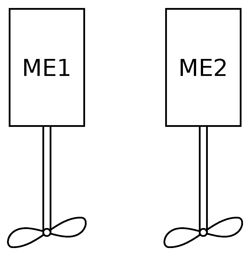
The ship is equipped with a hybrid-electric propulsion system. There is one propeller that is powered from a gearbox. The gearbox can be powered either from the main engine (ME), or from a hybrid shaft generator (HSG). The HSG converts electrical power from an electrical bus that can be powered from two identical diesel generators (DGs). There are several ways in which the propulsion system can be operated. In this case study, only the three predefined Machinery System Operational modes (MSO modes) Power Take Out (PTO), Mechanical (MEC) and Power Take In (PTI) are considered.

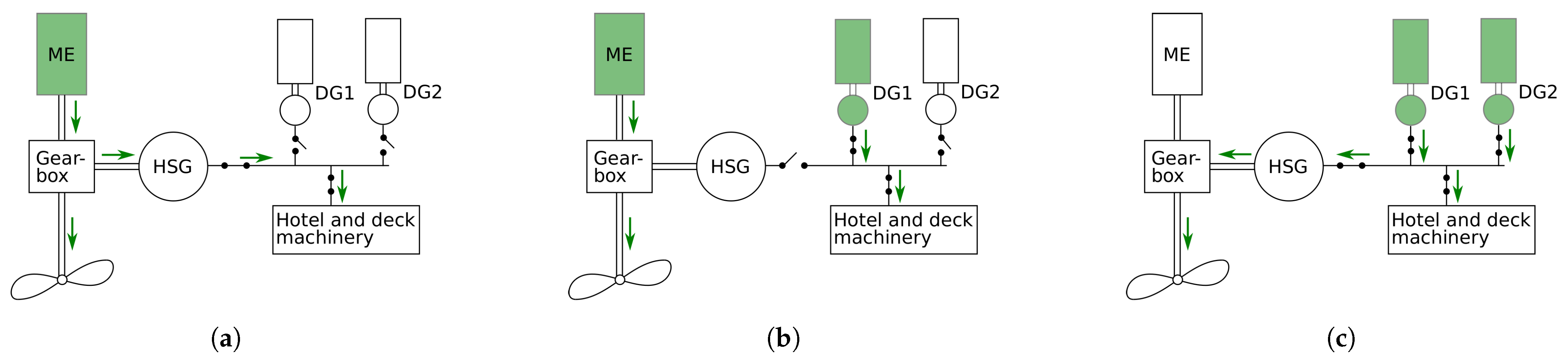
As illustrated in Figure 7a, PTO refers to a mode where the ME is responsible for the main propulsion, as well as auxiliary electrical loads. In this case, both DGs are offline and the HSG functions as a generator, transforming mechanical power from the gearbox to electrical power. In MEC mode, (see Figure 7b) the auxiliary electrical loads are served by one of the DGs instead of the HSG. Thus, the HSG is off, and all the power produced by the ME is used for propulsion. Finally, as seen in Figure 7c, PTI mode uses the DGs to provide power for propulsion. In this case, the HSG is acting as an electrical motor, transforming the electrical power from the DGs into mechanical power on the gearbox.

The main engine is a marine diesel engine with a maximum continuous rating (MCR) of 2160 kW, while the two diesel generators are rated at 590 kW each.

3.2. Risk Model Setup

Table 2. Description of the possible scenarios in each MSO mode.

MSO Mode	LOPP-Scenarios	Possible Restoration Scenarios
PTO	“ME stops”	“Restart ME”
		“Start DG1” AND “Start HSG”
		“Start DG2” AND “Start HSG”
MEC	“ME stops”	“Restart ME”
		“Start HSG”
PTI	“DG1 stops” AND “DG2 stops”	“Restart DG1”
		“Restart DG2”
		“Start ME”
	“HSG stops”	“Restart HSG”
		“Start ME”

presents the possible scenarios (consisting of a LOPP scenario and a set of possible restoration scenarios) that can occur in each MSO mode. The LOPP-scenarios and restoration scenarios are described in terms of triggering events and restoration events, respectively.

The expected rate of occurrence for each triggering event is presented in

Table 3. Overview of considered triggering events and rates of occurrence.

Triggering Event	ME Stops	DG1 Stops	DG2 Stops	HSG Stops
Failure rate	$3\times {10}^{-9}$	$6\times {10}^{-9}$	$6\times {10}^{-9}$	$2\times {10}^{-9}$

, and the restoration events and their parameters are given in

Table 4. Overview of restoration events and their statistical parameters.

Recovery	Start	Restart	Start	Restart	Start	Restart	Start	Restart
Events	ME	ME	DG1	DG1	DG2	DG2	HSG	HSG
Nominal prob.	1	0.4	1	0.5	1	0.5	1	0.8
Mean time	50	50	35	35	35	35	12	12
Std. deviation	1.4	1.4	1	1	1	1	1	1
Minimum time	20	20	14	14	14	14	3	3

. Here, the nominal probability refers to the probability of success of a recovery event given infinite amounts of time. The mean time, standard deviation and minimum time, are parameters in the restoration events success time, where mean time refers to the mean time given that it will start (i.e., assuming that the nominal probability is one). A lognormal distribution is assumed, where the minimum time parameter refers to a time interval. As an example, “Start ME” takes at least 20 s, according to the parameters in Table 4.

3.3. Environment Setup and Route Planning

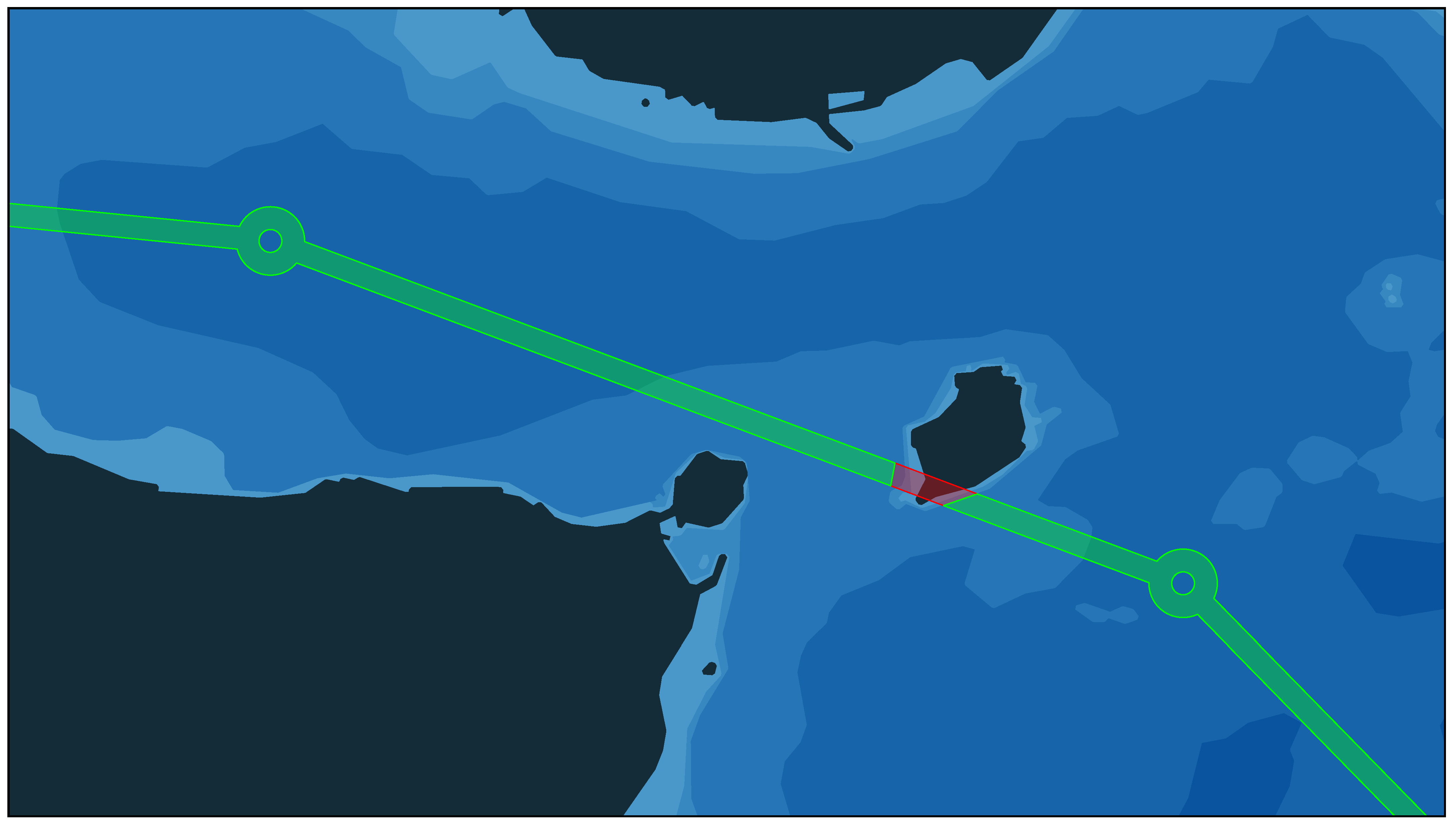
For proof of concept, a simple simulation environment is created using the ENC package SeaCharts [22] in Python 3.10. An area of approximately 14 square kilometers west-northwest of the Norwegian city of Ålesund is chosen for the simulation study, shown in Figure 8. This environment showcases an interesting scenario in which one may choose between two different paths on either side of an island, and is considered well suited for a proof of concept.

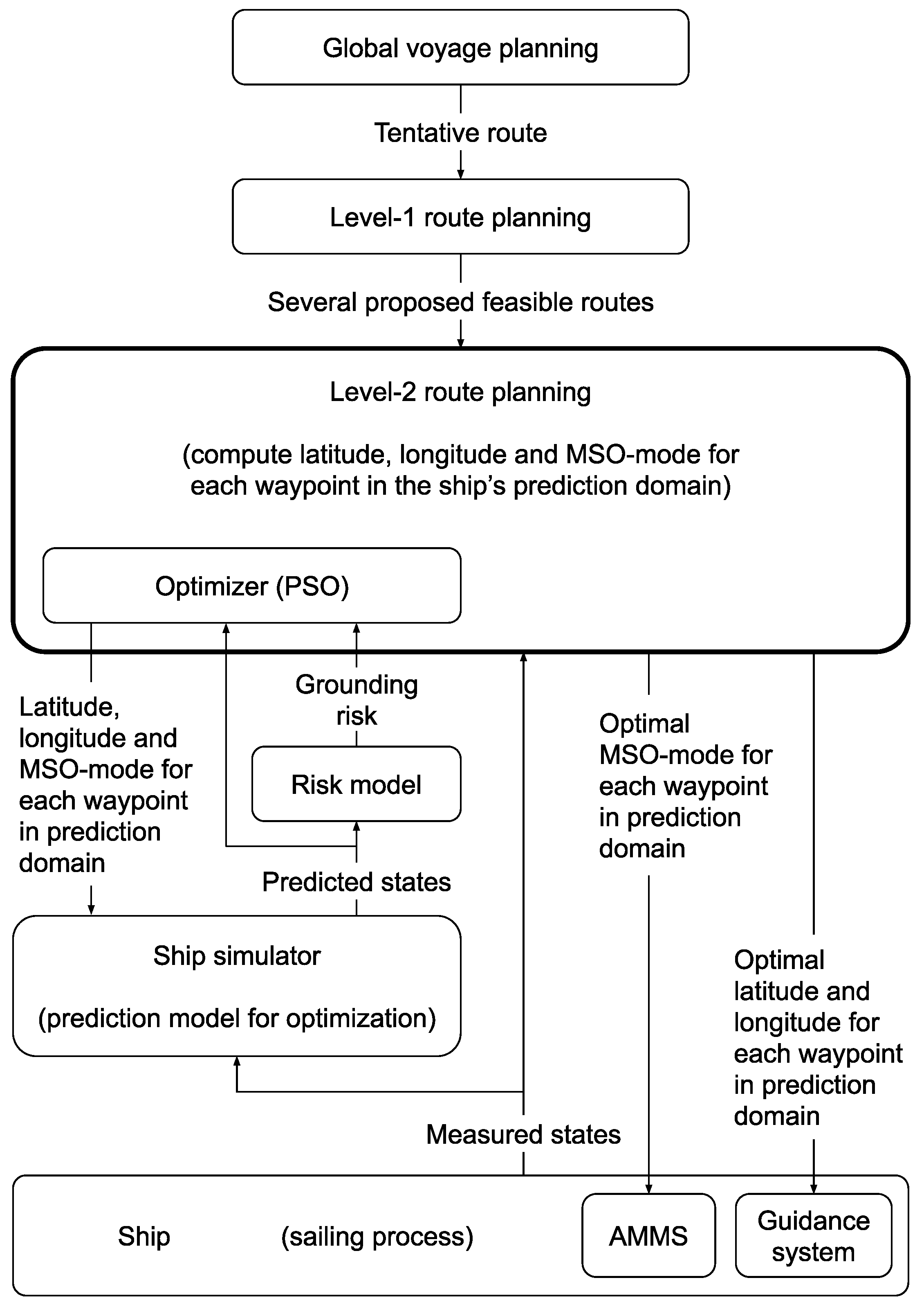
The tentative ship route or path to follow is shown in Figure 8 as green line segments connected by “links” at each given waypoint, as generated by the global voyage planner of Figure 1. Notice however how one of the green line segments are intersecting an island, highlighted by the red color where the island crosses the globally planned line segment. This setup is specifically chosen to demonstrate that if a planned tentative route is somehow inaccurate or incomplete such that grounding obstacles are present along the route, one may utilize e.g., the Level-1 route planner from [22] to generate alternative feasible routes on opposite sides of the obstacle in question. Moreover, one may analogously extend the anti-grounding algorithm to also encompass collision avoidance of dynamic obstacles, through e.g., the concept of (polygonal) adaptive safety domains [30] constructed around e.g., nearby vessels. Thus, it is argued that the approach shows significant flexibility and adaptability. Appendix A contains a summary of the planning algorithm, as well as a visual demonstration of each algorithm step.

Figure 9 shows the result of the Level-1 path planning performed on the ship route of Figure 8, as generated by Algorithm A1 from Appendix A. First, the green line segments are checked for intersections with any grounding obstacles in the environment, which in this case yields the red streak as shown in Figure 8. Second, the convex hull of the intersected grounding obstacle (island) is extracted, and an added buffer of a 50 $\mathrm{m}$ safety margin is applied in all directions from the obstacle exterior boundary, in addition to the already added 10 $\mathrm{m}$ buffer and vertex simplification process performed during the construction of the polygons of the SeaCharts ENC. This yields the two convex polygons highlighted around each of the islands south in the environment.

It is important to notice that one should be careful with this “hard” static safety margin. If this buffer around each grounding obstacle is too large, the subsequent path following or guidance controller may have trouble with navigation through extremely narrow straits, or one may even risk closing the strait in its entirety, losing the possibility of navigating through it as a route alternative. Thus, it is argued that the buffer should be somewhat conservative, and that the path following algorithm or controller is expected and required to be capable of operating in the interior of the feasible domain, as opposed to at the boundaries of hard constraints such as the grounding obstacle exteriors. Nonetheless, the Level-1 alternative route path planner is indeed a linear optimization algorithm operating on the vertices and line segments of each grounding obstacle polygons, essentially generating an approximate ship path to be used both during initialization and as part of the cost function of the Level-2 route planning optimizer of Figure 1.

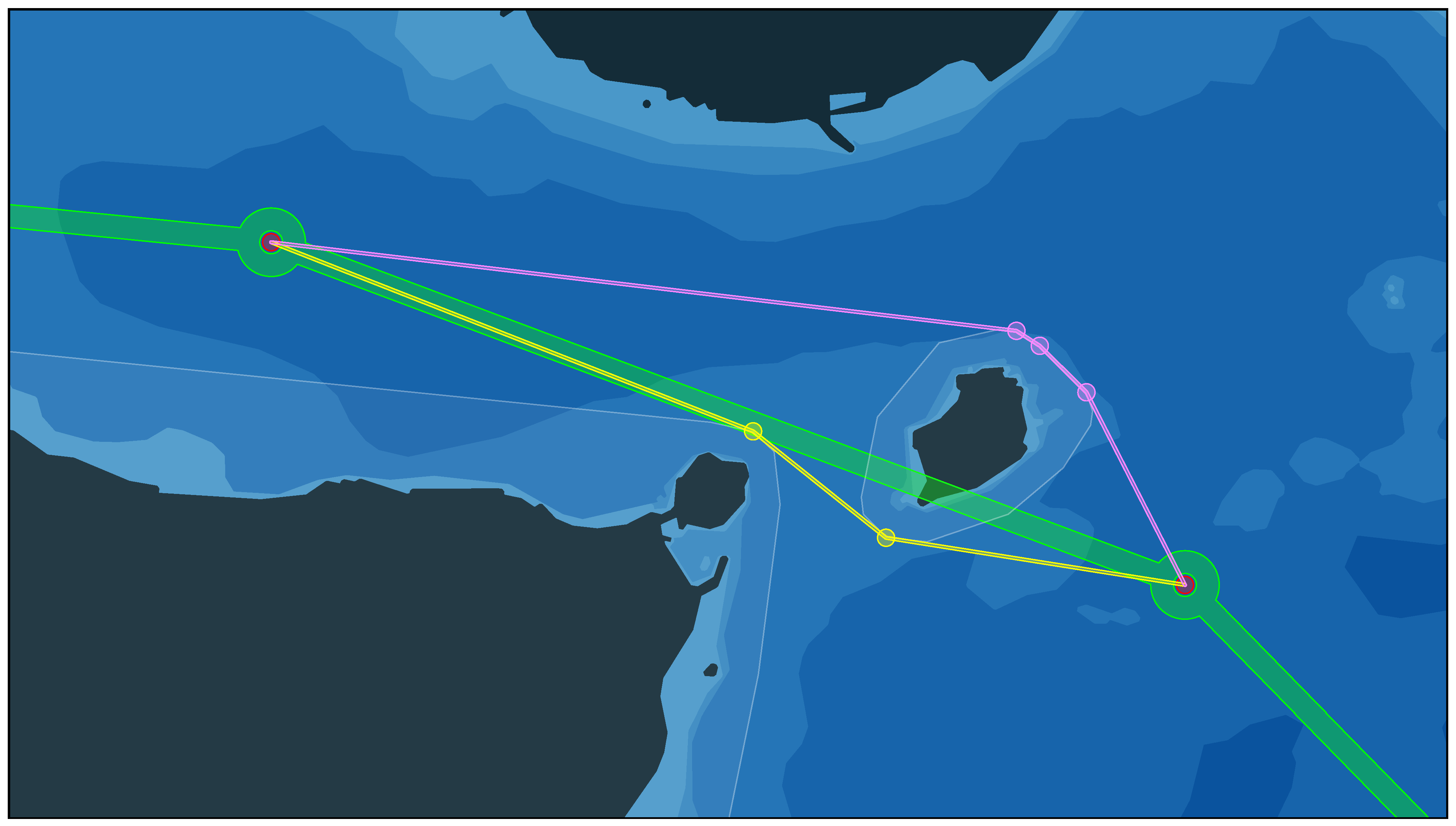
In Figure 9, the red disk within the path waypoint link to the east shows the start point of the simulation study. Conversely, the red disk to the west is the next target path waypoint. Algorithm A1 iterates through each of the grounding obstacle vertices, and checks if the point is visible (i.e., accessible along a straight uninterrupted line) from the reference point. The first reference point is thus the red east-most starting point, and the distances between each vertex visible from the reference location and the green line segment are measured. The visible vertex farthest away from the path is selected as the first alternate waypoint, and the process is repeated with each newly generated waypoint as the visibility reference location. This generates a new collection of line segments on each side of the grounding obstacle, and these alternative paths are in Figure 9 shown in yellow and pink. Notice how the generated yellow path originally intersected with the larger island to the south-west, which prompted another sub-run of the algorithm such that the new intersection is considered in the final path alternatives. See Appendix A for more details on this procedure.

3.4. Particle Swarm Optimization

The waypoint (route) optimizer used in this simulation study is a risk-aware Particle Swarm Optimization (PSO) waypoint planning algorithm which is extended, based on previous works [23]. Compared to other methods such as Model Predictive Control (MPC) [20], PSO is not subject to any special cost function construction or feasibility concerns in order to generate solutions (not guaranteed to be optimal). Thus, one may utilize highly discontinuous or discrete cost definitions, allowing for more complex general optimization.

The principle behind PSO is to randomly generate an initial swarm of N-dimensional solution particles, and repeatedly update the particle positions with respect to semi-random particle velocities based on their performance measured by the cost function. The technique is widely covered in the literature, and the reader is referred to previous works for more in depth background on PSO [23].

A simple demonstration case is shown in Figure 10, in which only the two-dimensional (2D) XY-coordinates of the path waypoints in the horizontal plane are optimized through purely distance-based and spatial costs from the ad hoc risk-aware implementation discussed in [23]. The same green line segments, start and target in red from Figure 9 are considered, as well as the newly generated route alternatives—here, shown in gray on each side of the smaller island.

The alternate paths are subsequently split into 20 sub-segments, corresponding to 19 waypoints shown in yellow and pink, respectively. The first line segment corresponds to the given start waypoint. These intermediate waypoints are used directly as the 2D particles to be optimized by the PSO, with respect to any nearby grounding obstacles. The cost function is a sum of simple path-related costs such as total path length and waypoint distances to the original path, as well as a simple risk-aware exponential function applied to the grounding obstacles [23]. The latter term weighs small distances between the ship position and nearby obstacles very highly compared to far-away locations, essentially adding a dynamic “soft constraint” which prevents the optimized path from crossing obstacles.

It is clear how the yellow and pink waypoints simulate increased risk-aware behavior with respect to the nearby islands, if followed by a navigation or guidance controller. Furthermore, one may also note how the lack of hard constraints keeps the problem well-behaved, even in the more narrow strait between the two islands shown in yellow. If, e.g., the safety margins discussed previously had been increased as a substitute for the distance-based “interior” cost inside the feasible region, one could end up with sharp and even infeasible paths between narrow straits such as the one shown. The magnitude of the obstacle avoidance costs are exaggerated for visibility in this proof of concept.

3.5. Risk Cost Formulation

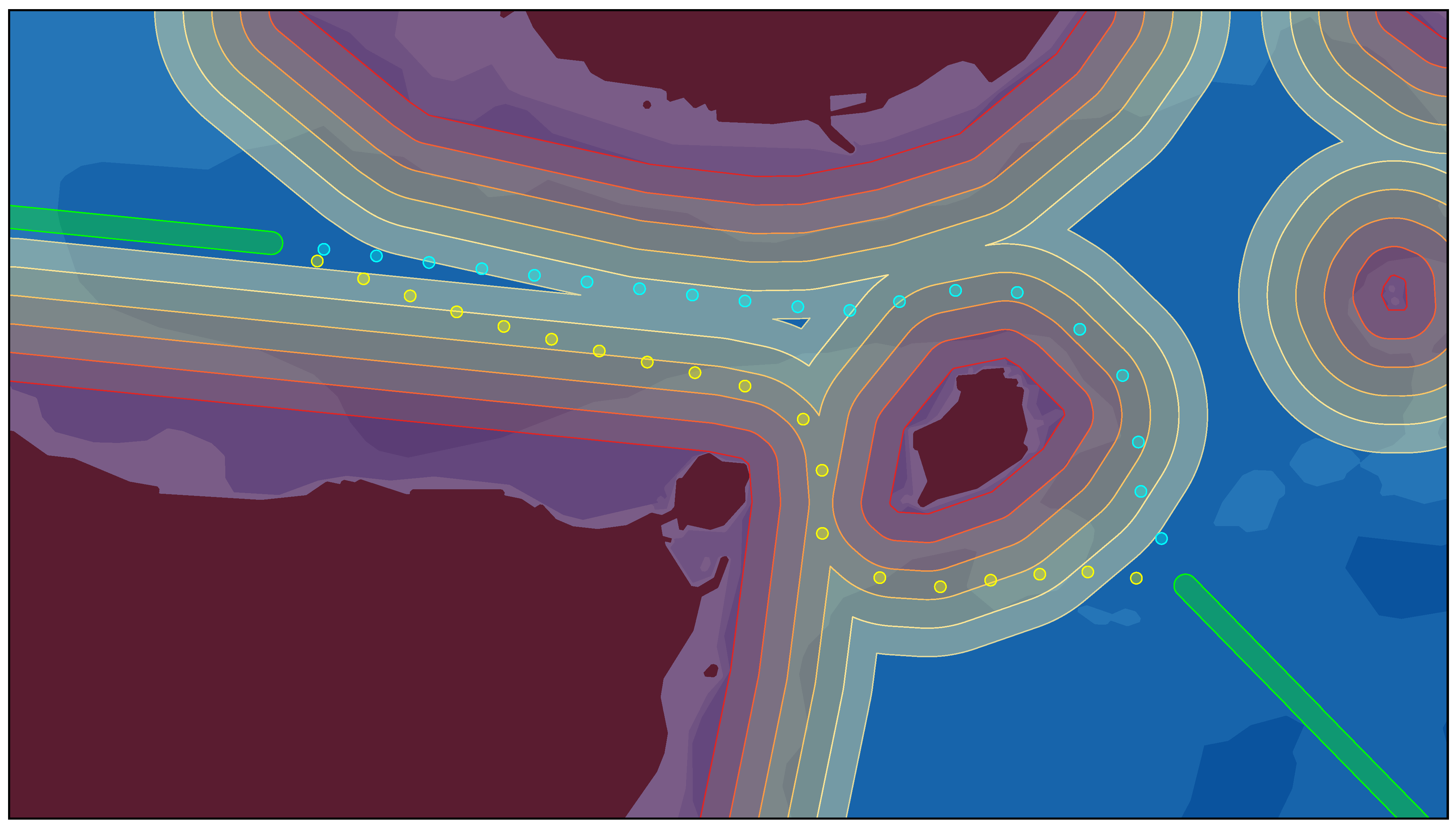
The formulation of the final risk-aware cost function is subject to many considerations. Figure 11 presents a visualization in which the same intermediate yellow and pink waypoints from the Figure 10 are shown in the colors yellow and cyan (replacing the pink for visibility), respectively. Here, the ends of the green line segments replace the initial route “links”, and denote the original red start and target locations. The increased risks simulated by the exponential term in the cost function is readily apparent from the overlapping contour polygons shown around each grounding obstacle, increasing in intensity and color from light yellow to dark red within the obstacle interiors. The optimized waypoints in yellow and cyan are seen traversing over or along the “hills and valleys” of the risk contours around the obstacles, and there is a strong correlation between the risk contour magnitudes and the resulting waypoints arrangement.

Obstacles previously hidden from sight also become apparent in this view, as every land area, shores and/or seabed depths more shallow than 10 m are included as (convex) red obstacle interiors. Thus, these obstacles also contribute to the spatial optimization, but are in this scenario negligible if sufficiently far away from the considered waypoints. This effect can be verified by comparing the colored intermediate waypoints with the previous alternate line path segments of Figure 10: There is no considerable discrepancy between the optimized waypoints and the Level-1 planned paths when no grounding obstacles are within some distance from the original path, as a direct consequence of the exponential nature of the risk cost term.

These distance-based risk awareness contours of Figure 11 resembles artificial potential (repulsion) fields, which is another popular approach used for path planning for e.g., unmanned autonomous vehicles. This method is however prone to becoming stuck in local minima and may show poor performance in narrow passages such as the isle strait considered here, and these issues must also be recognized and handled when using PSO. The sum of additional path-related costs are valuable in this regard, strongly related to the previous point with respect to the negligible divergence between the Level-1 routes and the optimized waypoints further away from obstacles: By enforcing large costs associated with straying away from the original path (as well as increasing the total path length), the (near-) optimal placements of each waypoint are semi-forced along the original path. This approach does however place more responsibility onto the Level-1 planner in order to achieve satisfactory solutions, which is considered appropriate following that the global planned path is already assumed to be near-optimal in this study.

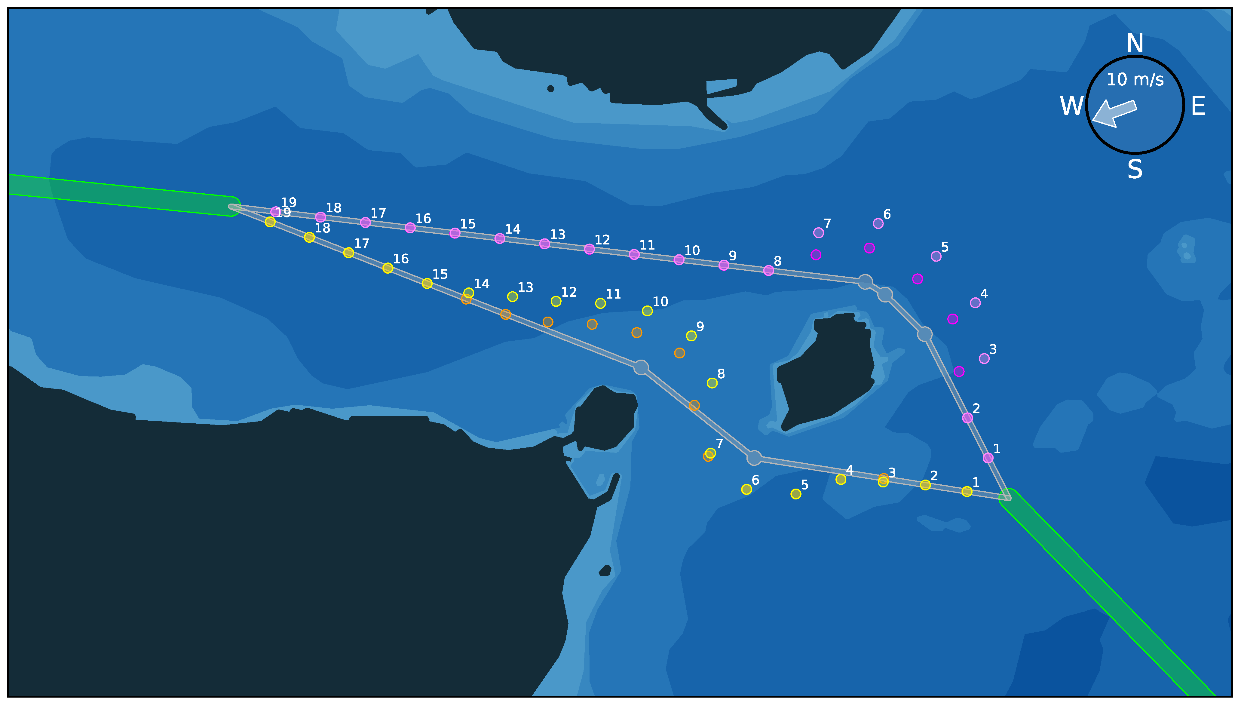
In previous works, a scalar cost with respect to environment (wind) disturbances was used in conjunction with the static distance-based grounding obstacle costs to account for the increased risks present when obstacles are located down-wind (or down-stream) of the ship [20,23]. Figure 12 shows a comparison view of the effect this extra cost term has on the waypoint distribution across each route alternative. The yellow and pink waypoint paths of Figure 10 are here denoted in orange and magenta, respectively, and the new resulting waypoints of each alternative including the added scalar product cost term are shown in yellow and pink.

For simplicity, only wind disturbances are included in the proof of concept demonstration. In the upper-right corner of Figure 12, the wind direction and wind velocity of the disturbance forces are shown as 250° and 10 $\mathrm{m}$/$\mathrm{s}$, respectively. It is clear how the scalar product of the wind direction and the direction to each grounding obstacle weighs more heavily onto the waypoint costs, effectively shifting them in approximately the opposite direction. Though the PSO algorithm is entirely sample-based and not gradient-based, the direction of the extra perturbations of the spatial waypoint locations are very similar, as expected. See the visualizations and discussions presented in the previous works for more details [20,23].

Some interesting effects are seen on a few waypoints. On the pink path, one can see how WP3 is more eastward, and WP7 is almost completely northward compared to their magenta counterparts, due to the scalar product of the closest point on the nearby grounding obstacle and the wind direction. Most notably, WP3 of the yellow path demonstrates a slightly unintended effect of using this risk cost formulation. Here, the wind direction (in this example) compared to the direction of the nearest potential point of grounding as seen from the ship, is such that the scaled extra cost of the exponential scalar product term is sufficient to noticeably move the waypoint southward unnecessarily. Though the risk cost scaling in these examples are exaggerated greatly for visual clarity, effectively resulting in less efficient routes around the islands, there is evident potential for improvements.

Thus, a new risk cost formulation is presented in this paper, which utilizes a ship model and the concept of TTG in order to produce more precise and appropriate waypoint planning solutions. It is argued that this cost formulation reflects realistic scenarios to a higher degree, more accurately incorporates the dynamics (i.e., the trajectory) of the ship, and is considered a natural addition to the cost function given the new scope which also includes machinery management considerations. The final cost function is presented in Section 3.9.

3.6. Path Following and Trajectory Control

The output of the Level-2 route planner of Figure 1 is ultimately given as input to the ship’s guidance system, which in turn controls the trajectory of the ship toward the resulting waypoints. Figure 13 shows an example simulation of trajectories produced by a line-of-sight (LOS) guidance controller, following the paths generated by both alternative sets of waypoints. Here, the speed of the ship is set constant, for simplicity. Most strikingly, the yellow trajectory is noticeably faster than its counterpart in pink. Its end position is readily seen in the figure being located farther along the path, after the same number of sampled time intervals.

In the example trajectories shown in Figure 13, the yellow trajectory is faster than the pink trajectory, but intuitively it does also involve higher levels of grounding risks—as apparent in Figure 11. This leads to the very purpose of this paper, and is indeed the main research question to be considered: How can both the efficiency and risk aspects of ship paths or trajectories be weighted such that the resource consumption is minimized during a successful mission execution, while simultaneously achieving safety?

3.7. Time-to-Grounding (TTG) Predictions

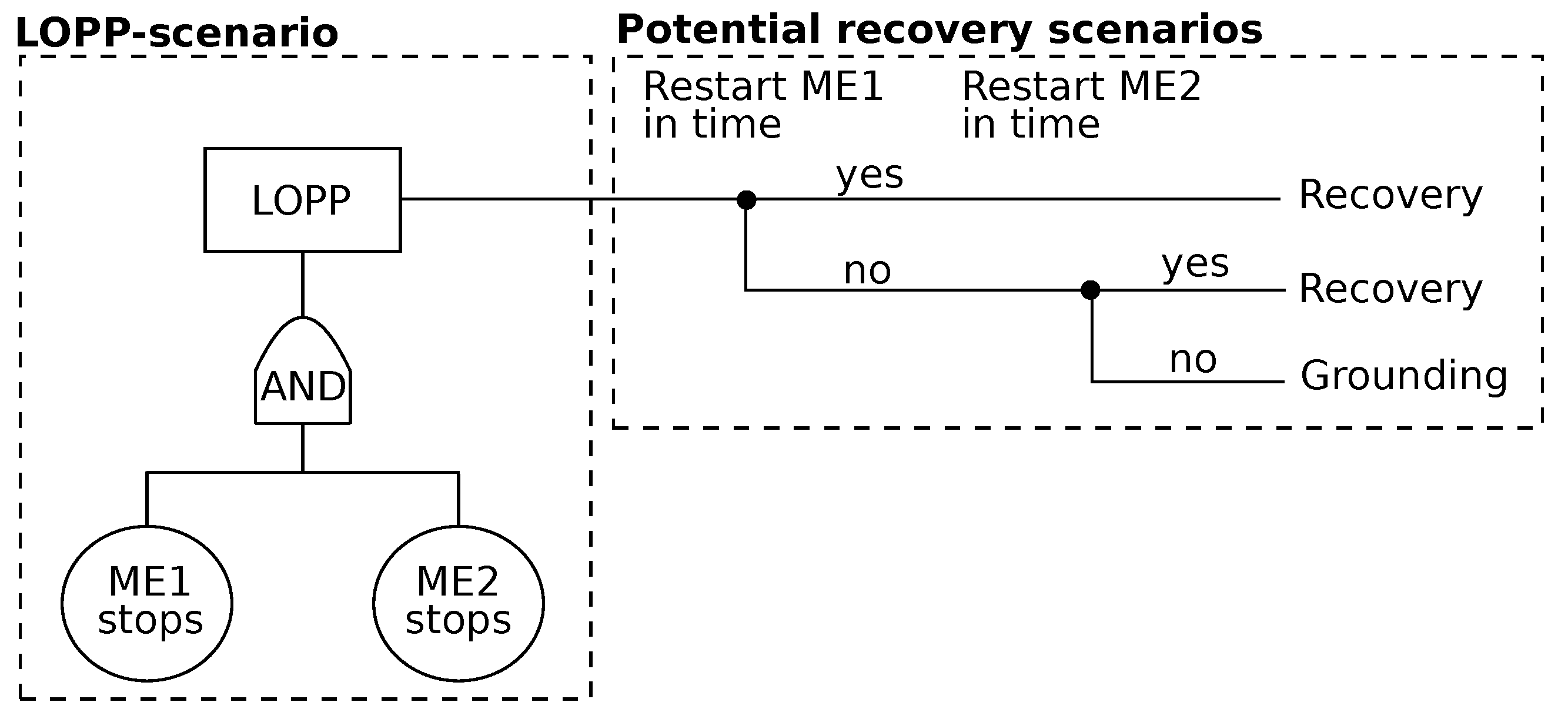
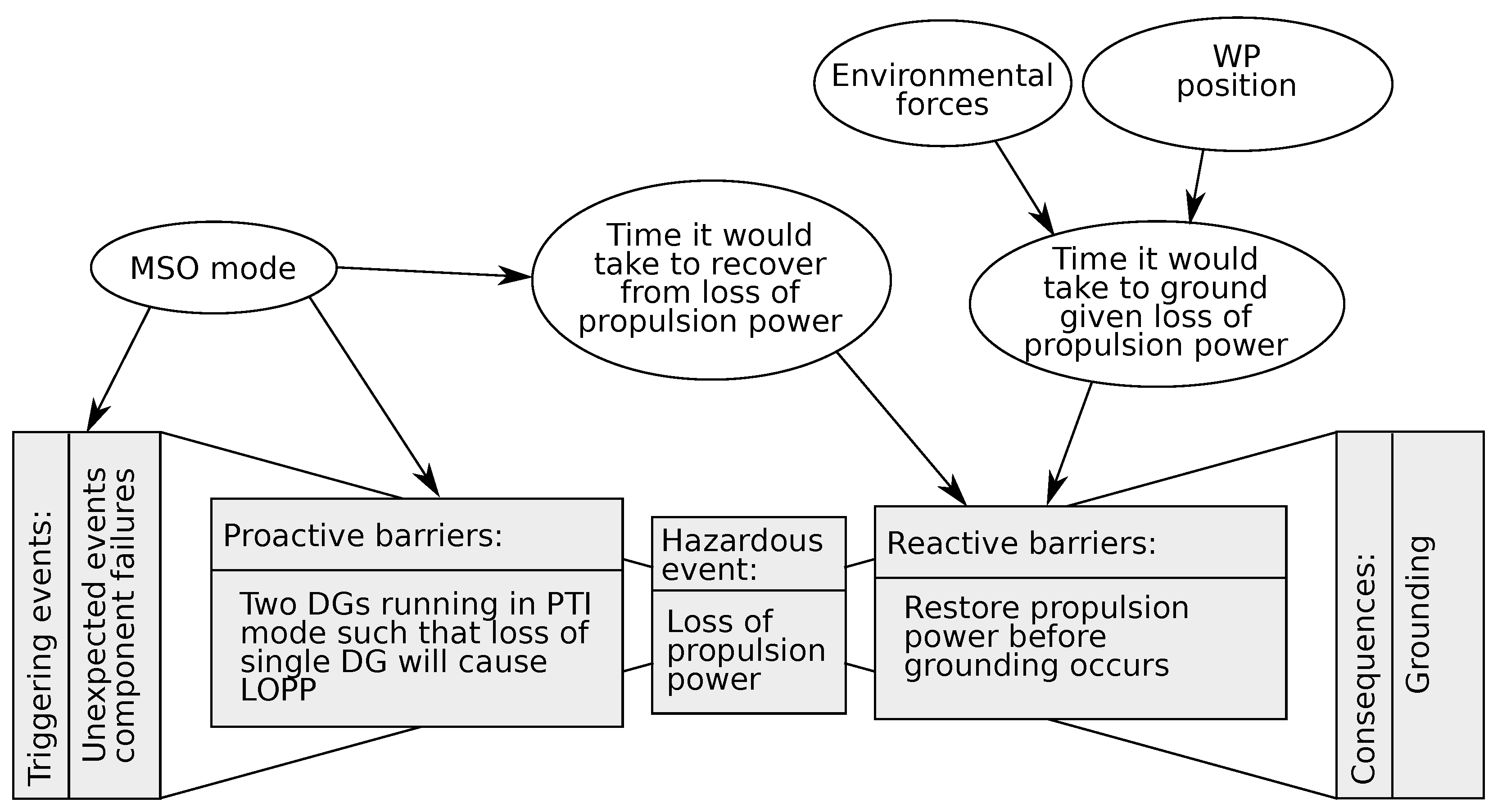
As noted in the discussion related to Figure 3 and Figure 4, the principle of “time-to-grounding” is simply to predict when (if) a ship would experience a grounding event if a LOPP (machinery failure) scenario occurs at a given time instant along the planned path, given the current or expected environment (weather) conditions.

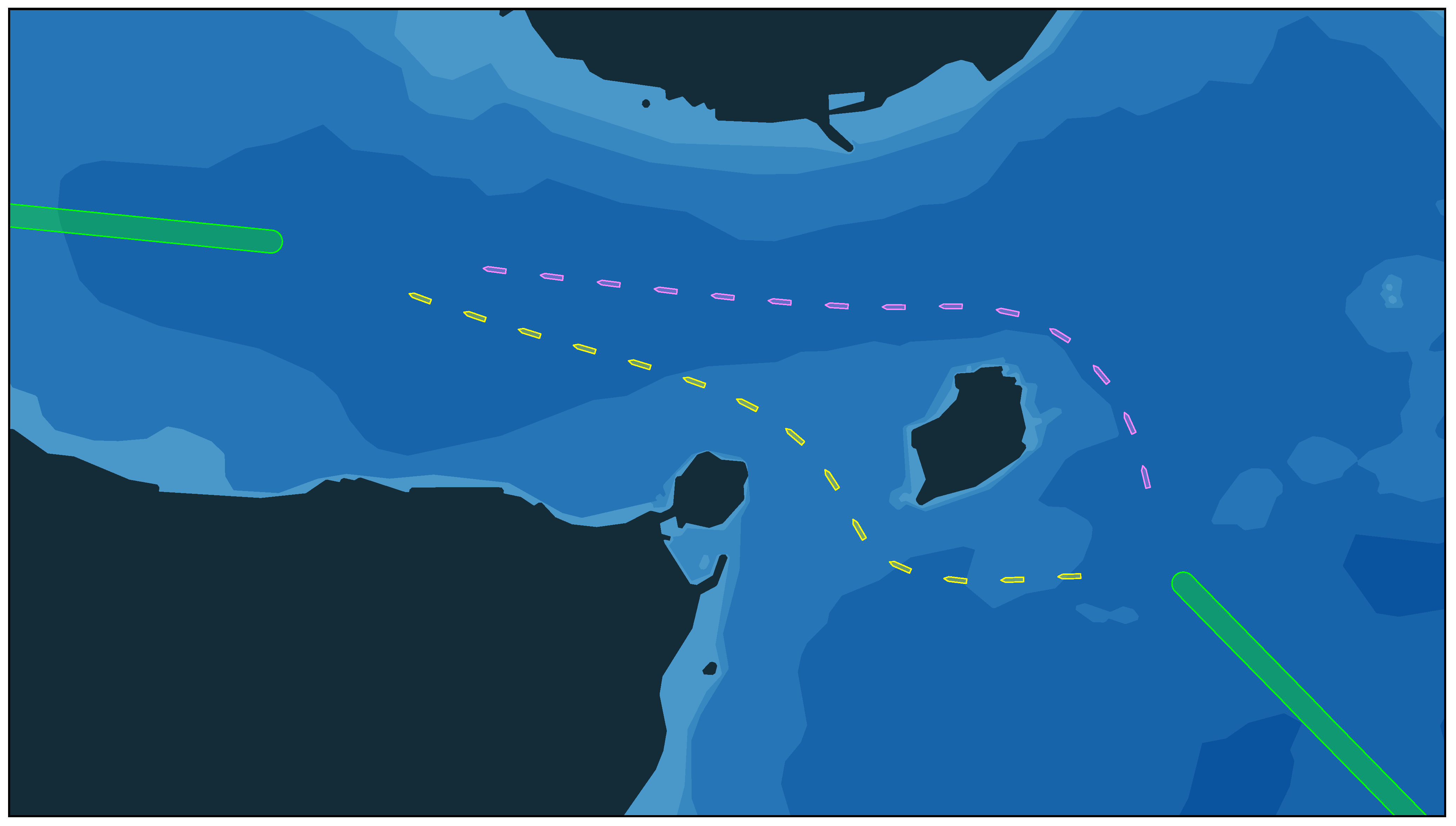
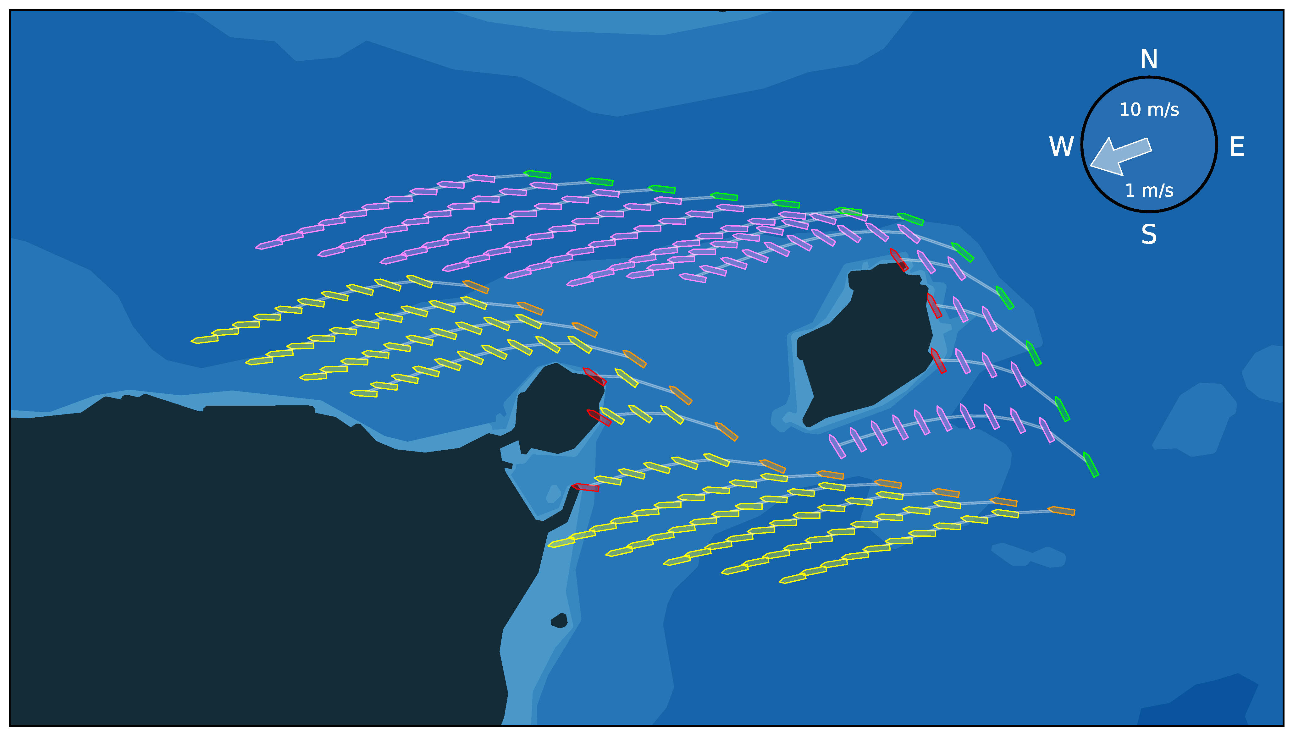
Figure 14 presents a demonstration of the TTG predictions. The wind velocity is 10 $\mathrm{m}$/$\mathrm{s}$, and the current velocity is 1 $\mathrm{m}$/$\mathrm{s}$. Here, the orange and green collections of ship poses are not simulation trajectories, but rather the ideal ship poses defined for each waypoint distributed evenly along the original paths. This shows how an initial ship yaw angle or heading is needed for each (ideal) waypoint in order to predict TTG. The angles are calculated using the angle between the previous and the next (neighboring) waypoints, for each individual waypoint. The yellow and pink colored ship poses denote the predicted trajectories during a LOPP scenario corresponding to each ship pose of the orange and green routes, across a horizon of 10 $\min$.

The predicted future trajectories with no propulsion and steering are simulated by the ship model, and include the ship dynamics and initial ship speed before loss of propulsion power. As expected given a wind direction of 250°, the ship in the orange trajectory is predicted to drift south-west toward the south-west island, and the ship in the green trajectory would firstly hit the smaller island. Moreover, as the accumulated probability of grounding only increases (and is defined) given that a grounding event has not occurred, the future predictions are ended if any part of the ship intersects with a grounding obstacle. These intersections are shown as red ship poses. Note that the red grounding events may be asynchronous with respect to the regular sampling intervals of predicted ship state (pose), across the LOPP scenario horizon.

3.8. MSO Mode Selection and Fuel Consumption

The TTG predictions are used to inform the optimization during the PSO run, i.e., to select the most suitable MSO mode as well as the waypoint locations during optimization. This is due to the fact that each MSO mode have different fuel consumption rates when active, and have different restoration properties. The resulting time values of the TTG predictions are subsequently translated into grounding probabilities, and then expected costs through the rate of failure probabilities and restoration rates of Table 2, Table 3 and Table 4. These costs are ultimately weighted against all other costs defined by the path following cost function, and the PSO outputs three-dimensional (3D) solution particles consisting of the X and Y coordinates of each waypoint, and the selected MSO mode to be used for the following time interval.

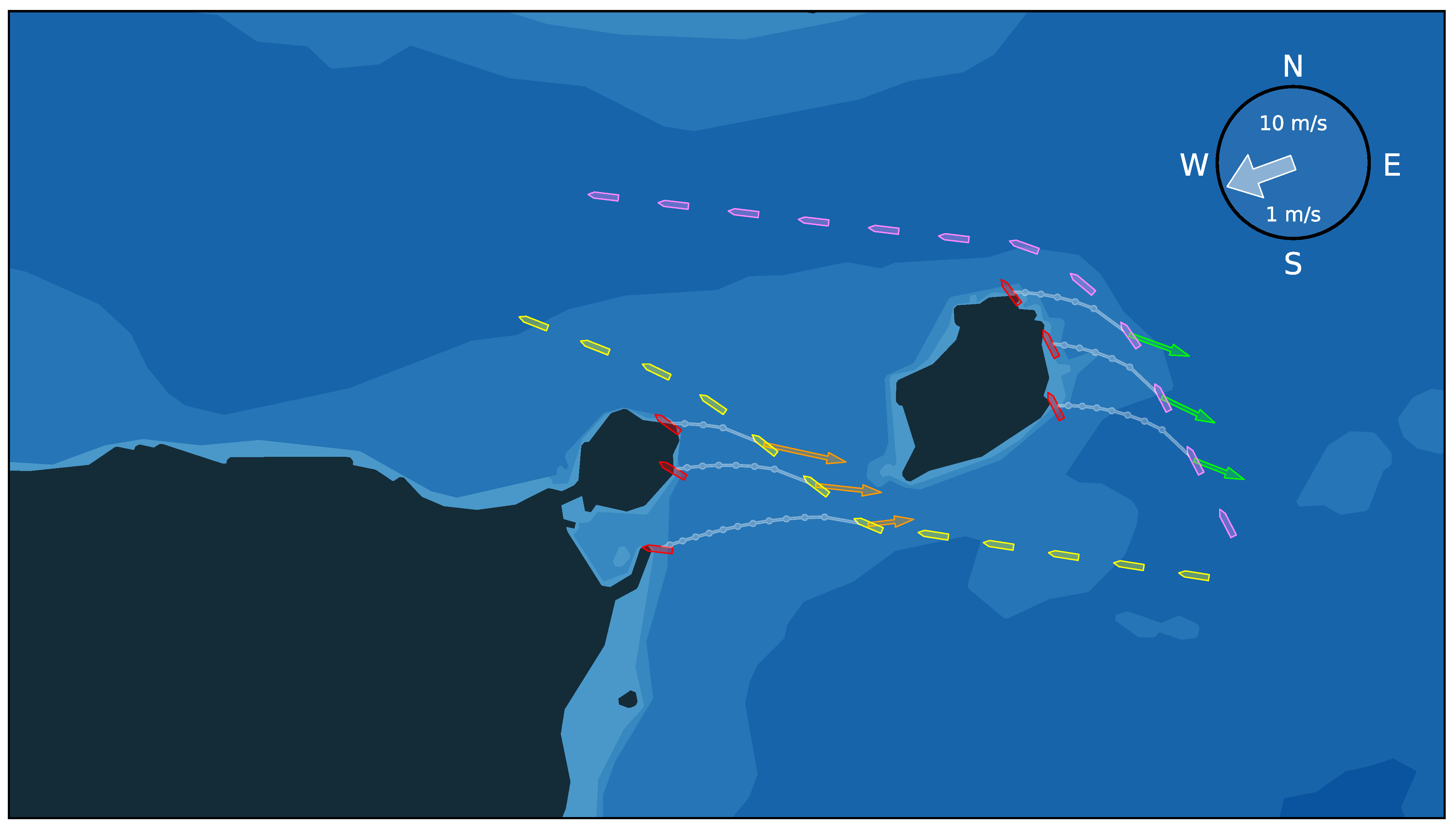
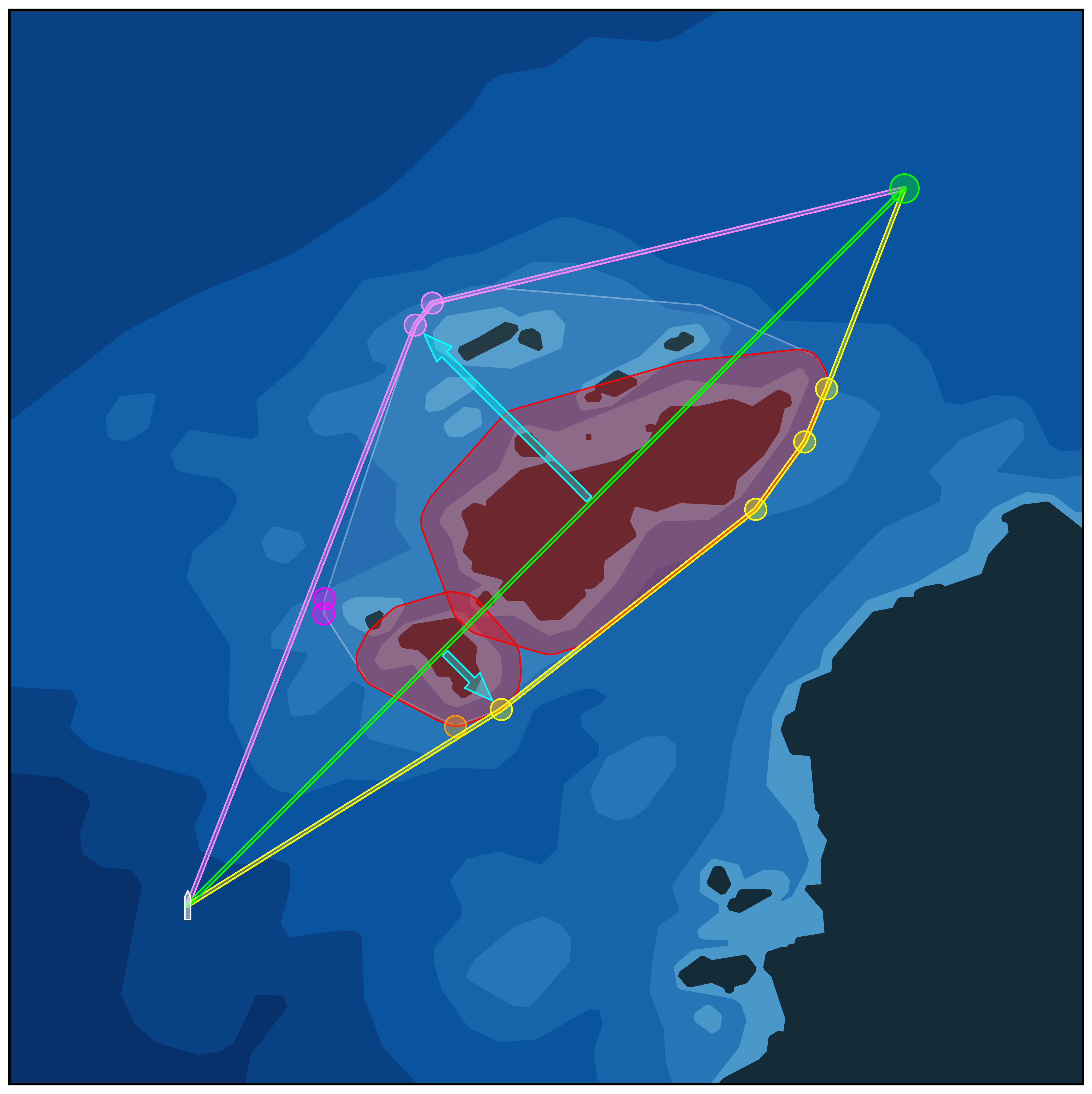
Figure 15 presents an alternative view of the ideal sailing routes and LOPP blackout predictions of Figure 14, in which additional directed arrows denote how the 2D cost gradients of the waypoint locations in the horizontal plane are affected by the TTG predictions and resulting estimated costs. The altered locations of the optimized waypoints would in turn increase the total fuel consumption, assuming that the original path is near-optimal. It is intuitive that since the risks for a grounding event occurring increases along the direction of the wind disturbance, a purely spatial cost function would move the waypoint locations away from the predicted points of impact [20,23]. However, in this work, the MSO mode selection also plays an important role.

In this figure, the trajectories are unchanged for the purpose of conceptual demonstration and comparison to later results. For this example, both trajectories experience proximity to higher grounding probabilities for an approximately equal amount of time. However, in general, this is not necessarily the case, and the fuel consumption along the complete trajectories are highly dependent on both the specific MSO mode selected, and the accumulated time spent in the mode. Thus, it may sometimes be more economically prudent to simply move the route waypoints further away from the grounding obstacles, as an alternative to disrupt the machinery to go into another (i.e., safer but also more costly) MSO mode. This joint combination of spatial path optimization and operational mode cost minimization during operations is considered the novel contribution of this work.

3.9. The Complete Cost Function and Simulations

Based on the discussions and intermediate results of the previous sections, the final complete cost function is formulated as follows:

$$C_k(\mathsf{\varpi },m)=C_{path}(\mathsf{\varpi },k)+C_{grounding}(\mathsf{\varpi },k,m)+C_{mso}(\mathsf{\varpi },k,m)$$

(11)

$$C_{path}(\mathsf{\varpi },k)={\mu }_1\left|\right|\mathsf{\varpi }-{\mathsf{\varpi }}_k^{ref}{\left|\right|}^2+{\mu }_2{\left(\left|\right|\mathsf{\varpi }-{\mathsf{\varpi }}_{k-1}^{ref}\left|\right|-\left|\right|\mathsf{\varpi }-{\mathsf{\varpi }}_{k+1}^{ref}\left|\right|\right)}^6$$

(12)

$$C_{grounding}(\mathsf{\varpi },k,m)=C_G\left({\mu }_3\sum _{\sigma \in O}{e}^{-d_{min}(\mathsf{\varpi },\sigma ){\zeta }_1}+{\mu }_{4}P\left(G\right)\right)$$

(13)

$$C_{mso}(\mathsf{\varpi },k,m)=C_{consumption}·{\mu }_5\left|\right|\mathsf{\varpi }-{\mathsf{\varpi }}_{k+1}^{ref}\left|\right|$$

(14)

where ${\mathsf{\varpi }}_k=P(x,y)$ is a 2D waypoint corresponding to the k^th line segment along a route alternative, and x, y, k and m are the x- and y-coordinates of a waypoint, the line segment number and the selected MSO machinery mode, respectively.

The second term of $C_{path}$ is raised to a larger (even) power than the first to more strongly encourage distributing the waypoints with equal distances between each other, compared to being close to the ideal reference waypoint along the route. ${\sum }_{\sigma \in O}{e}^{-d_{min}(\mathsf{\varpi },\sigma ){\zeta }_1}$ is the total sum of the negatively scaled minimum distances to every grounding obstacle raised to the power of e, which serves as an exponential barrier function for nearby grounding obstacles irrespective of the heading of the ship or any disturbances.

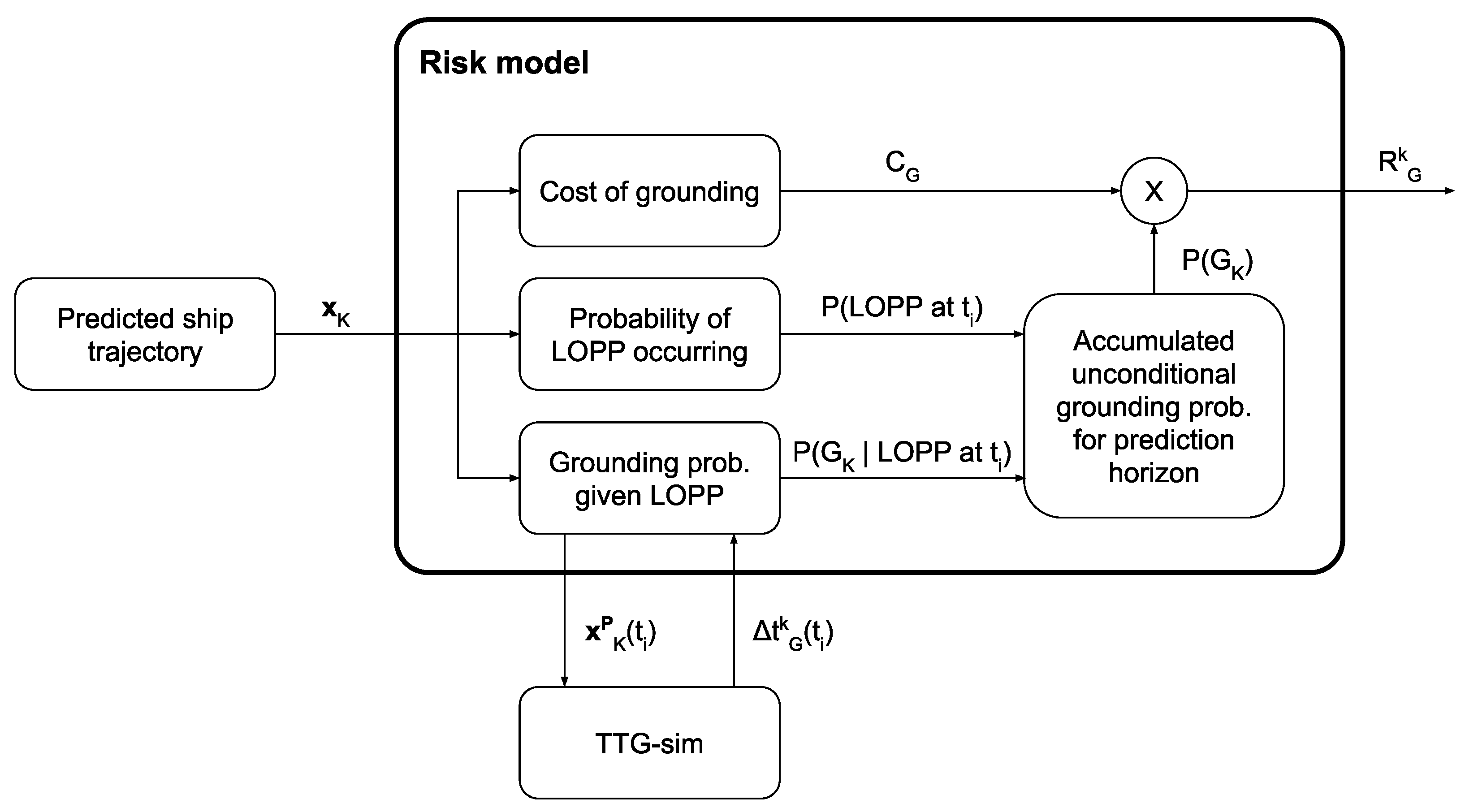
$P\left(G\right)$ is the accumulative grounding probability function from (5), and $C_{consumption}$ is the estimated fuel cost per meter traveled. For simplicity, it is for (11) assumed that the variable costs defined in (10) are held constant for the entire optimization horizon, i.e., $C_G$ is static based on a set of assumptions related to the current surrounding environment. The reference waypoints ${\mathsf{\varpi }}^{ref}$ denote the ideal waypoint locations evenly spread across all line sub-segments along a route alternative if left completely unaltered by grounding risk costs, i.e., $C_{path}=C_{grounding}=0$ (see the pink waypoints 8 to 19 in Figure 12). In this work, the PSO setup used 30 candidate particles in each particle swarm (one for each of the 20 line segments), and was run for 100 iterations. The following hyper-parameters of the PSO was used: The inertia weight was set to 0.75, the cognitive weight was 1.0, the social weight was 2.0, and the velocity limit was 1.0.

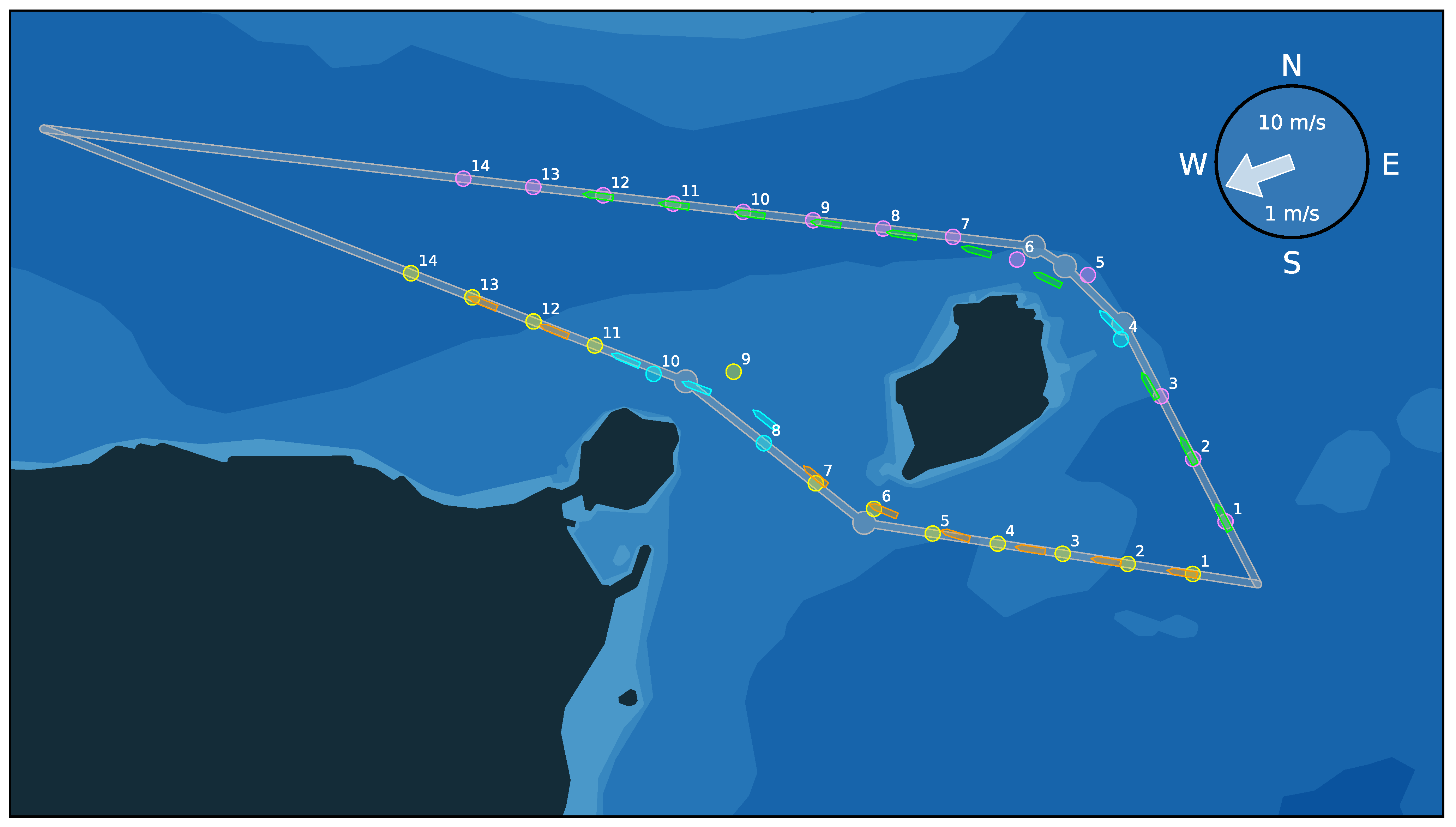
Using the path following guidance controller, the resulting optimized WP distributions and trajectories of each route alternative are shown in Figure 16. The green trajectory follows the resulting PSO route in pink, and the orange trajectory follows the yellow route. The target ship heading each time interval is calculated by drawing line segments between the optimized waypoints, and extracting the target coordinates by intersecting the resulting path by a circular horizon radius of 200 $\mathrm{m}$. Thus, the generated ship trajectory is entirely independent of the distance between each optimized waypoint of the PSO, and the smoothness of the path to follow may be improved simply by increasing the number of waypoints to optimize.

The cyan waypoints on both routes denote where the most robust but costly MSO mode is selected for a specific WP interval (MEC), and the cyan ship pose shows where the ship has this mode active during its voyage in order to reduce the expected costs of grounding due to the TTG simulations. All other waypoints are given their original colors when using the most economical MSO mode (PTO). These results show how e.g., WP10 of the yellow route and WP6 of the pink route are allowed closer to the nearby obstacles compared to e.g., Figure 12 (demonstrating the approach of previous works [23]), as the cost function now integrates and considers the ship dynamics.

Moreover, it may be noted that the MEC mode is still selected also for the line segment following WP9, for the purpose of demonstration—the MSO mode selection algorithm may utilize more advanced mode management mechanisms than simply choosing the most economical at each interval. It is also apparent that WP9 in this example is moved away from the nearby obstacle, leading to the normal PTO mode being selected. Though such mode switching generally is unwanted due to additional startup/switching costs, this outcome is included here for completeness only; a more sophisticated behavior may be tweaked and fine-tuned as desired.

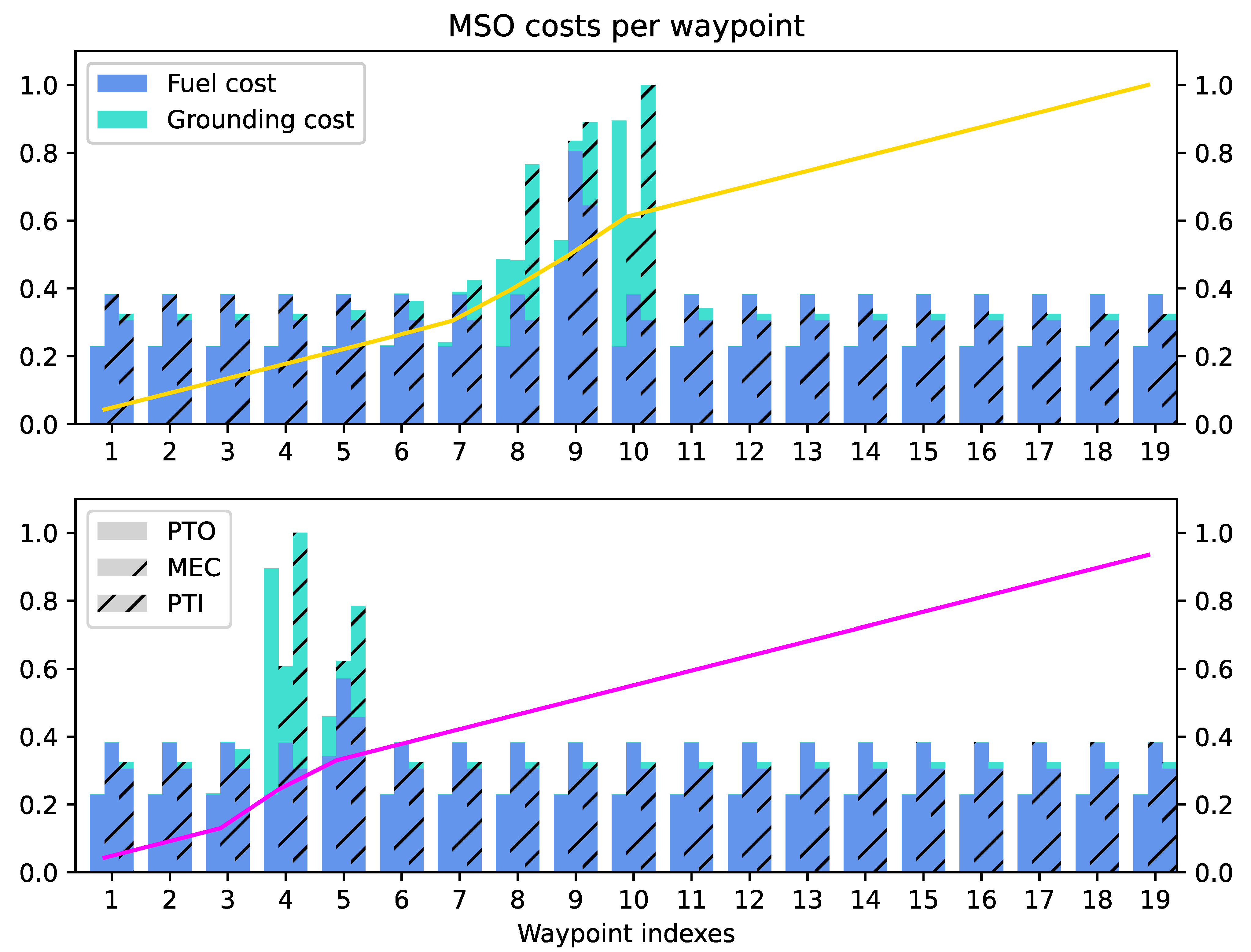
Graphs of estimated (expected) grounding and fuel costs of each route, as well as the total accumulating costs along each alternative, are presented in Figure 17. Expected costs for grounding shows the ${\mu }_4$ term of $C_{grounding}$ (13) for each waypoint, and are shown as blue bars. It may be noted that as the scaling coefficients for grounding events are constant in this work, the value of the blue bars may serve as proxy visualizations for the grounding probabilities P(G) experienced during the TTG simulations of each waypoint, i.e., a taller bar means a larger expected rate of grounding occurrences, which are noticeably different for each mode due to their inherent restoration capabilities. Expected (additional) costs for added fuel consumption with respect to the optimal path are denoted as the green bars on top. The three different MSO modes PTO, MEC and PTI are denoted by zero, halved and fully streaked bars, respectively. The total heights (sum) of these bars are the total expected costs of each MSO mode selection, for each waypoint.

It is apparent how each MSO mode are proportionately related to different fuel cost rates and grounding risk probabilities (due to different restoration rates), e.g., PTO has a lower fuel cost but also a larger grounding risk scaling associated with it, compared to that of MEC. During optimization, the mode with the lowest total cost is simply chosen for each route line segment between optimized waypoints. Note that the cost coefficients used in this work are ad hoc for a proof of concept, and are consequently only meaningful relative to each other. Thus, both Y axes are normalized between 0 and 1.

Definite indications of increased grounding risks and thus expected costs are clearly visible for WP 6, 7, 8, 9 and 10 for the yellow path, and WP 3, 4, and 5 for the pink path. This is in line with the visual information shown of the environment in Figure 16, i.e., the nearby grounding obstacles affect the costs as expected. One may also note that, despite being as close to the obstacles as the mentioned points, WP 11 of the yellow path and WP 6 and 7 of the pink path are not affected in the same way, due to the general direction of the TTG predictions as a result of the given disturbances. Moreover, there is a noticeable difference between the expected fuel cost of WP 9 in the yellow path compared to its two neighbors. This also corresponds to the visually apparent location shift of the waypoint, in which the increased fuel costs of moving the waypoint in this situation were less expensive than the expected grounding costs for this specific interval. One possible explanation for this result may be that the expected TTG for this interval is less than the shortest minimum time required for all available restoration events, which significantly increases the grounding risk for that initial waypoint location.

The yellow and pink lines are the accumulating costs of each respective route, used to select the most efficient route. Ultimately, the pink route with its resulting green trajectory was chosen due to the lowest total expected cost across the entire (predicted) simulation run. This result shows how the fastest route may not always be considered the most cost-effective within a specific environment and set of conditions, and thus a slightly longer but more effective and/or safer route is generated and selected as the optimal choice.

4. Discussion

It is recommended that the methodology and proof of concept presented in this paper should be implemented and tested in a practical implementation in future research. Moreover, testing of different combinations of various PSO hyper-parameter settings, number of particle candidates and number of iterations should be investigated and assessed in order to achieve improved performance.

The structure and tuning of specific terms in the complete cost function have a significant impact on the resulting solutions. In fact, the behavior or final waypoint distribution across each route alternative is by definition entirely dependent on both the cost function formulation and its inherent weighting coefficients. As such, the choices made with respect to the individual terms of the cost function must be thoroughly assessed. The sub-parts of (10) may in future research be weighted dynamically with respect to the ship state or predicted states. However, $C_G$ is in this proof of concept given a constant value for simplicity.

The $C_{path}$ term (12) consists of only path-related costs, which keep the waypoint distribution close to the original route alternative (the first term) as well as distributing the waypoints evenly across the full length of the original route. The values of both the exponents and its weights (${\mu }_1$, ${\mu }_2$) is however highly flexible, and may be adjusted to accommodate various levels of strictness with respect to the path following aspect of the cost function as deemed most fitting by the human operators. Furthermore, it may be noted that though the TTG simulations are time-dependent during the LOPP simulations, $C_{path}$ is not. This is a deliberate choice made in order to enable utilization of parallel computing techniques, due to each waypoint being fully independent from all other variable waypoints during optimization as a result of only using the ideal (static) reference waypoints ${\mathsf{\varpi }}^{ref}$ in this cost term. However, it may be argued that the PSO optimization instead may be structured such that the cost of each WP is dynamically calculated with respect to the best known costs of each PSO WP neighbor instead of the static references. Though this structure is not parallelizable, it may potentially achieve even more optimal waypoint distributions in future works.

Next, the $C_{grounding}$ term (13) is comprised of both the exponential anti-grounding costs as well as the weighted TTG-based accumulative probabilities of grounding if a LOPP event occurs. Though these terms are quite different in their form and the resulting effects of each consequently are difficult to compare directly, both are considered necessary to formulate as such in order to achieve desired behavior. The first term is included solely to serve as a strong barrier function for the purpose of extra safety, which may override any insufficient tuning or if any unexpected or unaccounted for events may occur. Thus, the term is exponentially defined, even though the resulting costs close to grounding obstacles are difficult to define explicitly or compare to more practical probability- and expected costs-based terms. This formulation may also be thoroughly examined in later research.

Similarly to the path-related cost formulation, the $C_{mso}$ term (14) is based on fuel consumption with respect to the next ideal waypoint, as opposed to a perhaps more intuitive parameters such as total distance traveled, or time. This somewhat indirect form is also chosen in order to enable parallel computing, eliminating the need to include the variable waypoints during optimization, which vastly reduces the computational complexity. It is argued that though the resulting cost is not accurate in terms of actual fuel consumption estimated during the voyage, it is a useful measure of how much extra consumption is required for any waypoint change with respect to the ideal route alternative. This is considered appropriate within the scope of this study, due to the pre-computed reference path being assumed near-optimal.

Note that the implementation and cost formulation in this work do not include any additional cost terms for switching of MSO modes, nor any considerations of time delays or other time-dependent variables related to e.g., cold-starting an engine. These factors were not handled in this proof-of-concept study, but are however considered natural and appropriate additions to further research efforts or industrial applications.

There are many uncertainties related to both the measurement of states and predicting future states, and the models used to calculate these states. The management of such uncertainties is an important consideration of optimization problems such as the one presented in this paper. In general, one may add additional safety margins to mitigate potential damages if the accumulated errors due to uncertainties lead to an accident. In addition, the models used for environmental factors were kept simple in this study. Future work should also include and implement more comprehensive and accurate models for calculation of environmental forces or physical effects, such as varying ocean depths and disturbance dynamics (winds, waves and currents) in order to reduce the amount of uncertainties present in the system.

Lastly, the results as presented in Figure 16 and Figure 17 are highly subject to the tuning of the cost function coefficients, and should be acknowledged as such. Moreover, the results are assessed and validated by human evaluation of the behavior of simulated trajectories in a challenging scenario, which is subjective and subject to bias. The environment and cost function weights of this study are to a large degree chosen or established in order to show-case interesting behavior relevant to the proposed methodology, and is consequently biased toward this particular configuration. The method for tuning and assessment should thus be comprehensively investigated in future works.

5. Conclusions

This paper proposes a methodology and proof-of-concept simulation study which utilizes PSO for simultaneous selection of machinery operational modes combined with waypoint re-planning based on grounding risks calculated from spatial distances and “time-to-grounding” simulations, such that both safety and efficiency may be considered more accurately during optimization compared to previous works. The results show that a slower route with respect to time and distance traveled may still be considered more cost-effective in terms of expected costs when also recognizing grounding risks along a route.

There are nevertheless several limitations that could be addressed in future work. As mentioned, the method could be extended for collision avoidance with dynamic obstacles and following the traffic rules at sea. Moreover, while the choice of PSO as an optimization engine is effective, other methods such as genetic algorithms should be considered as well. Although it is straightforward to define safety margins to account for uncertainty in models and input data, a more systematic method for determining the uncertainty levels and setting the safety margins would be useful. For an industrial implementation, hazard analysis should be used to obtain a more complete overview of the scenarios that potentially can lead to accidents, and to gain more insight into which factors may affect the risk, and how. The proposed framework fully supports the implementation of a more comprehensive risk model, and is thus considered a promising approach to serve as the foundation to future works on joint machinery management and autonomous navigation.