Markovian-Jump Reinforcement Learning for Autonomous Underwater Vehicles under Disturbances with Abrupt Changes

Abstract

This paper studies the position regulation problems of an Autonomous Underwater Vehicle (AUV) subject to external disturbances that may have abrupt variations due to some events, e.g., water flow hitting nearby underwater structures. The disturbing forces may frequently exceed the actuator capacities, necessitating a constrained optimization of control inputs over a future time horizon. However, the AUV dynamics and the parameters of the disturbance models are unknown. Estimating the Markovian processes of the disturbances is challenging since it is entangled with uncertainties from AUV dynamics. As opposed to a single-Markovian description, this paper formulates the disturbed AUV as an unknown Markovian-Jump Linear System (MJLS) by augmenting the AUV state with the unknown disturbance state. Based on an observer network and an embedded solver, this paper proposes a reinforcement learning approach, Disturbance-Attenuation-net (MDA–net), for attenuating Markovian-jump disturbances and stabilizing the disturbed AUV. MDA–net is trained based on the sensitivity analysis of the optimality conditions and is able to estimate the disturbance and its transition dynamics based on observations of AUV states and control inputs online. Extensive numerical simulations of position regulation problems and preliminary experiments in a tank testbed have shown that the proposed MDA–net outperforms the existing DOB–net and a classical approach, Robust Integral of Sign of Error (RISE).

1. Introduction

Compared to Remotely Operated Vehicles (ROVs), Autonomous Underwater Vehicles (AUVs) may respond faster based on feedback from some perception modules or positioning systems and can thus enhance their performance in tasks, e.g., exploration, surveillance, cleaning bridge piles, and placing a heavy cover on a leaking oil well [1,2]. However, AUVs in shallow waters are often disturbed by inevitable strong disturbances. This research studies the control problem of stabilizing a control-input-saturated AUV under unknown excessive external disturbances [3,4,5]. Due to some events, the dynamics of external disturbances involve abrupt variations, making the transient performance of AUV unsatisfactory.

Much effort has been devoted to rejecting or attenuating disturbances in control problems since the 1980s. In particular, robust control [6], H-infinity control [7], adaptive control [8,9,10], and high-order sliding mode control [11] have been explored and used in industrial applications. In [12,13], Disturbance OBservers (DOBs) are used to estimate the lumped effects of unknown disturbances and uncertain dynamics models based on state observations and control inputs. From the first appearance of DOBs, many advanced ones have been studied, such as high-order disturbance observers for time series expansion and nonlinear systems [14,15].

Many control methods based on DOBs have since been developed, among which is the disturbance accommodation control [16,17,18]. Mismatched disturbance has been studied in the continuous and finite time regulation problem in [19], and values and multi-order derivatives of the disturbances are estimated to augment and stabilize the system via Lyapunov stability theorems.

However, the above-mentioned improvements in feedback controllers might fail to guarantee stability when the controlled system is subject to control saturation [20]. Small gain theorem might be explored in this case. However, it requires sufficiently accurate dynamics models, which are difficult to obtain for AUVs subject to various disturbances. These DOB-based approaches are effective when the disturbances are bounded and sufficiently small (compared to the actuator capacities) [21]. When the disturbance forces acting on the AUV frequently exceed the thrusters’ capacities, the AUV can not be easily stabilized [3,22].

An ideal controller has to consider the (even saturated) controls’ long-term effects on attenuating future disturbances; therefore, it is better to optimize the performance over a future time horizon, leading to constrained optimal control problems. Model Predictive Control (MPC) can deal with control input saturation and is thus an ideal candidate [20,23]. However, MPC usually requires a sufficiently accurate prediction model of the system [24], which might be unavailable due to the existence of disturbances in dynamics. Continuous-time MPC with a disturbance observer was proposed for disturbed systems in [25], where the disturbance estimations are utilized to adjust the prediction of the system output online, and an accurate AUV model is required. However, the latter is difficult to obtain, and, in addition, the disturbances are functions of time, which are unknown and difficult to measure via sensors. Another challenge associated with MPC is the computational burden of solving constrained optimization problems in real time at each time step.

The unknown dynamics models of AUV and the disturbances inhibit MPC approaches. These limitations of MPC and DOB-based controllers have led to DOB-nets [22], enabled by recent advances in Reinforcement Learning (RL). Model-free RL is adopted in this study since it does not require an explicit system model and can naturally adapt to noises and uncertainties [26]. Most existing RL methods build the controllers and critics in the domain of the AUV state space (the pose-velocity space). As a result, such RL can only capture the dynamics by the mappings between AUV state spaces, while the disturbances are functions of time and can not be described by mappings between AUV state spaces [27]. The unmodeled dynamics are treated as noises, which are further assumed to be independent and identically distributed (i.i.d.). Following this formulation, the noises are quite large and make the AUV system unstable, as shown in [22].

The key to this issue is to find an appropriate domain to define the dynamics model of the disturbed AUV and, thus, the controller, leaving the remaining unmodeled effects as noises of small moments. Many existing works model disturbances as superpositions of many harmonic oscillations [28]. In [22], model-free RL has been applied to reject excessive disturbances by modeling the control problems of the disturbed AUV via a set of unknown Partially Observable Markovian Decision Processes (POMDPs). The transition function (i.e., disturbed AUV dynamics) of each POMDP is heavily affected by disturbances. The input domain of the controller is built on the AUV state and the encoding of disturbance estimations in a future time horizon.

However, the work in [22] assumes that each POMDP has fixed harmonic oscillations, ignoring the fact that the disturbance dynamics may have abrupt changes. The dynamics of external disturbances are subject to abrupt changes due to events, e.g., a large vessel passing by, strong currents hitting underwater structures or oil well eruptions. Therefore, AUV’s transient performance regarding these abrupt changes is unsatisfactory.

In this paper, it is shown that disturbances with varying characteristics can be modeled as a Markovian Jump Linear System (MJLS), the study of which has drawn a lot of attention. MJLS is found in many practical applications, and it aims to describe abrupt system variations caused by environmental changes. The disturbances are modeled by MJLS for multiple disturbances in [29], where the transition matrix is partially known. A disturbance attenuation controller is constructed to achieve asymptotically stable performance. Singular Markovian-jump systems have been investigated in [30], where infinitely unobservable states are treated as unknown inputs. In addition, the approaches in the existing literature (e.g., [31,32]) do not consider control saturation, which widely exists and becomes an issue when the controlled objects are subject to excessive disturbances. To the best of the authors’ knowledge, the stabilization problem of a control-input-saturated system subject to completely unknown and Markovian-jump disturbances has not been addressed.

Contribution: This study proposes a new RL approach referred to as MDA–net, which consists of a disturbance-dynamics-characteristics observer network (referred to as observer network) and an optimal controller network (referred to as controller network). Compared to DOB–net, MDA–net has three improvements.

(i)

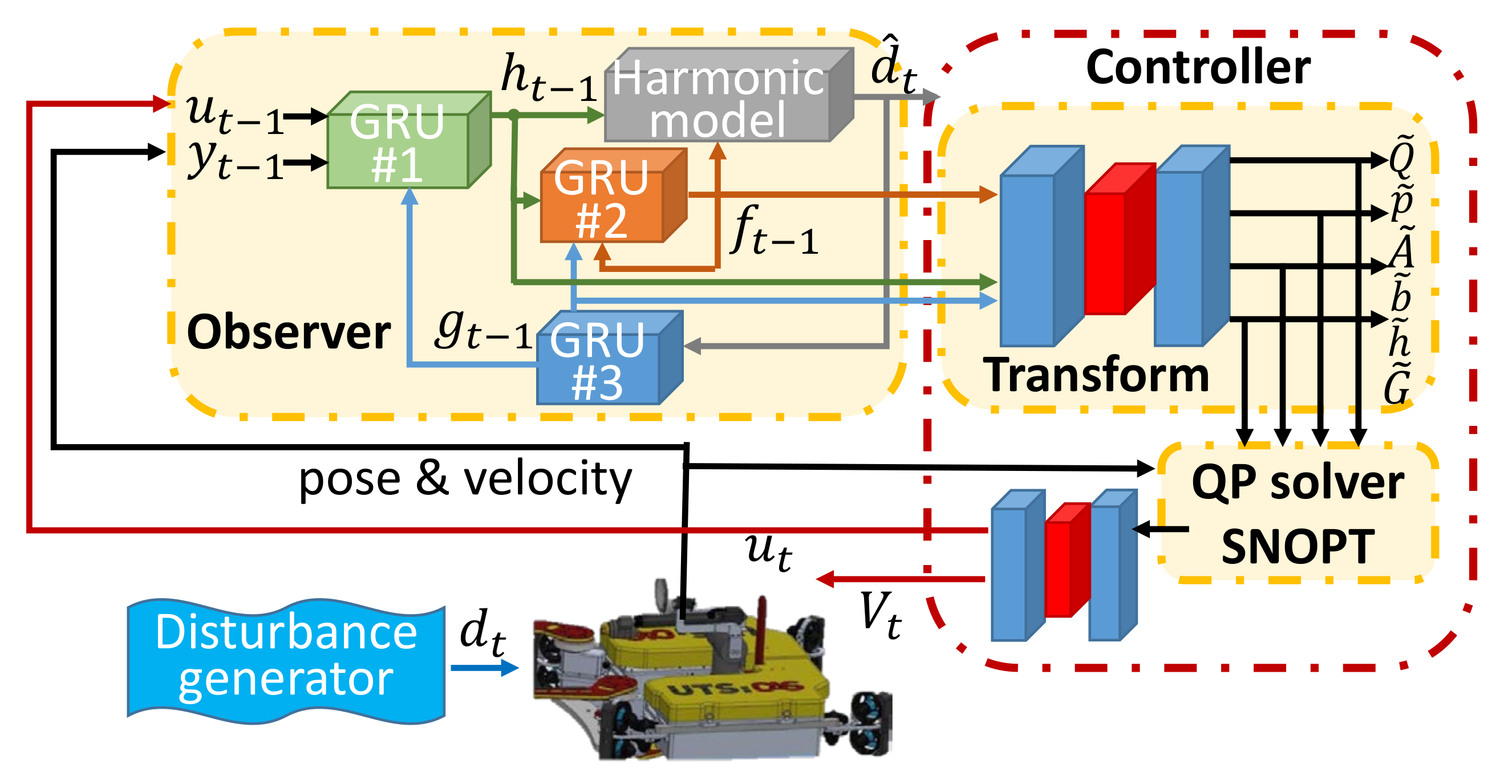
Different from the one in DOB-nets, the new observer network aims to learn the characteristics (i.e., frequencies, phases, and amplitudes) and their transition dynamics (i.e., properties describing Markovian-jump characteristics). The goal of this observer network is to provide the feature description of the in situ disturbed AUV system dynamics to the control network.

(ii)

A two-step learning approach (module learning and end-to-end learning) is adopted, which is regularized by the process of the disturbance prediction built on the disturbance harmonic model (the superposition of multiple disturbances). The observer network outputs a feature representation of the quadratic optimization problem in the encoding space, which is further referred to as the problem feature in the remainder of this paper. It is natural to train a solver (a controller network) that receives these problem features and outputs control signals. However, it is difficult to learn a solver of optimization problems purely from data. A Quadratic Programming (GP) solver is embedded in the controller network.

(iii)

In this paper, the gradients of the optimization over the problem features are established based on the sensitivity analysis of optimization regarding the QP solver and are then used to train the controller network together with the critics.

In the remainder of this paper, the formulation of the position regulations problems is given in Section 2, and then the previous work DOB–net is reviewed in Section 3. After that, Section 4 and Section 5 present the MJLS formulation and the proposed MDA–net, respectively. Section 6 summarizes the implementation details and the results from the numerical simulation and experiments in lab conditions. The limitations and potential improvements are discussed in Section 7, followed by conclusions in Section 8.

2. Problem Formulation

The position regulation problem arises from many underwater applications. The stabilization of AUVs is particularly important to inspection or intervention tasks where the AUV platform is free-floating and affected by the disturbance. AUV platforms often have sufficiently large restoring forces and can thus be kept horizontal. Therefore, the pitch and roll motions are not considered. The desired restoring forces can be achieved by designing the distance between the buoyancy center and the mass center. The surge, sway, heave, and yaw motions of the AUV platform are heavily affected by the excessive disturbances and thus require a proper controller.

Let $\mathbf{q}\in {\mathbb{R}}^3\times SO\left(2\right)$ denote the AUV position and heading, and the AUV velocities and accelerations $\dot{\mathbf{q}}$ and $\ddot{\mathbf{q}}$ are in the tangent space ${\mathbb{R}}^4$ of the manifold. It is assumed that q and $\dot{\mathbf{q}}$ are obtained from the perception system, e.g., Simultaneous Localization And Mapping (SLAM). In clean water with steady illumination, cameras can be used, while in other cases, an onboard multi-beam sonar can be used, as reported in [33]. The dynamics of the disturbed AUV are given as

$$\mathbf{M}\left(\mathbf{q}\right)\ddot{\mathbf{q}}+\mathbf{C}\left(\dot{\mathbf{q}}\right)\dot{\mathbf{q}}+\mathbf{D}\left(\dot{\mathbf{q}}\right)\dot{\mathbf{q}}+\mathbf{g}=\mathbf{u}+\mathbf{d},$$

(1)

where $\mathbf{M}\in {\mathbb{R}}^{4\times 4}$ denotes the inertia matrix, $\mathbf{C}\in {\mathbb{R}}^{4\times 4}$ denotes the matrix of the Coriolis and centripetal terms, $\mathbf{D}\in {\mathbb{R}}^{4\times 4}$ denotes the matrix of the drag force, and $\mathbf{g}\in {\mathbb{R}}^4$ denotes the vector of the lumped gravity-buoyancy forces. As pointed out in [34], it is quite difficult to measure these terms, which depend on the flow density and velocities. Therefore, in this study, these matrices and vectors are unknown to the controller.

In the studied problems, the disturbances are represented by their equivalent forces acting on the AUV platform. In the remainder of this paper, “disturbances” and “disturbance forces” are used exchangeably, and they are denoted by $\mathbf{d}\in {\mathbb{R}}^4$. The control $\mathbf{u}\in \mathcal{U}$ is saturated at bounds $\overline{\mathbf{u}}=max\left(\mathcal{U}\right)\in {\mathbb{R}}^4$ and $\underline{\mathbf{u}}=min\left(\mathcal{U}\right)\in {\mathbb{R}}^4$, where max and min are dimension-wise operators, and $\mathcal{U}\subset {\mathbb{R}}^4$ is a compact set of control. For simplicity, the bounds on each dimension of u are independent of each other. This assumption might not be true if the total power from all thrusters is restricted by the AUV’s power supply.

Definition 1

(Excessive External Disturbances). The disturbances are called excessive if their forces d acting on the AUV frequently exceed the control saturation $\overline{\mathbf{u}}$ and u.

The external disturbances in this study are excessive to the actuators’ capabilities (see Definition 1). Definition 1 only makes sense if the control inputs and the disturbance forces enter the AUV system from the same channel. In other cases, a similar definition might be explored by mapping the control inputs and disturbances into the same channel. In a real AUV system, the disturbance forces may enter the system from a different channel as control inputs u. The experimental results have shown the formulation in Equation (1) is reasonable.

Problem 1

(Optimal Control Problem). Obtain a controller that outputs actions u to the system (1), such that an objective function is maximized in an episode under disturbances of randomly generated and abruptly changed characteristics. System (1) is discretized in time, and the objective function is defined as the discounted sum of the collected rewards,

$$J=\sum _{\tau =0}^{T-1}{\gamma }^{\tau }r\left({\mathbf{x}}_{\tau }\right),$$

(2)

where $r\left({\mathbf{x}}_t\right)\triangleq -{\mathbf{x}}_t^{T}R{\mathbf{x}}_t$, ${\mathbf{x}}_t$ is the AUV state at time t, T denotes the number of time steps in an episode, and γ ∈ [0, 1) is a discount factor that prioritizes the near-term rewards [35].

The optimization of Equation (2) is subject to Equation (1) and control saturations $\overline{\mathbf{u}}$ and u. More importantly, the obtained controller should be applicable to Problem 1 with various randomly generated and abruptly changed disturbances.

3. Previous Work: DOB–net

The control problems of the heavily disturbed AUV cannot be precisely described by a single POMDP in the AUV state space. Augmented state spaces have been studied to better describe the dynamics of the disturbed AUV. Based on the assumption that recent states and actions together encode the transition functions of a POMDP at the visited states, a history-window control approach has been developed, and it takes in as inputs a number of most recent states and actions [36]. Similarly, the disturbed AUV dynamic system has been modeled as a multi-order Markovian chain in [37]. However, it might be difficult to determine the number of orders. A small number of orders might not rediscover the POMDP characteristics, while a large number of orders make the training and generalization of the trained policy challenging.

The DOB–net approach, proposed in [22], is built on the classical actor-critic architecture, as described in Figure 1. DOB–net utilizes hidden states from Gated Recurrent Units (GRUs) to encode the transition function of the multi-order Markovian chain. DOB–net consists of an observer network and a controller network, as shown in Figure 1. The observer network is built upon GRUs to mimic the dynamics involved in DOBs and the dynamics of time series prediction. The controller network outputs the control signals and critic values, as required byA2C. Since the controller is also a function of the AUV state, state x is aggregated with the hidden state from the observer network.

The DOB–net (the observer network and the controller network) is trained in an end-to-end manner through interactions with the disturbed AUV systems [38,39,40]. The procedures of training and testing contain a number of episodes, where each episode contains T time steps. DOB–net outperforms the existing approach RISE. However, in [22], the disturbances considered have constant characteristics in each episode. The abrupt changes in these disturbances are not considered. As a result, the transient performance in abrupt events is poor.

4. Markovian Jump Linear System

This section shows that by modeling disturbances as the superpositions of multiple harmonic oscillations, Problem 1 can be modeled as a Markovian Jump Linear System (MJLS). With this modeling, it is reasonable to embed a QP solver in the controller network. This layer of the QP solver is different from regular layers (activation layers or hidden layers); it involves running QP to solve for solutions. The details of this QP layer are introduced in Section 5.

As pointed out in [41], the harmonic disturbance in the channel of the control input is given by the exogenous systems,

$$\begin{array}{c}{\mathbf{d}}_t=\mathbf{V}\left[{\mathbf{s}}_t\right]{\mathit{\omega }}_t,\\ {\mathit{\omega }}_{t+1}={\mathit{\omega }}_t+\mathbf{W}\left[{\mathbf{s}}_t\right]{\mathit{\omega }}_t+\mathbf{G}\left[{\mathbf{s}}_t\right]{\mathbf{e}}_t,\end{array}$$

(3)

where ${\mathbf{s}}_t$ is a discrete-time Markovian process, ω is the internal state of the disturbance, and ${\mathbf{e}}_t$ is square integrable over time horizon $[0,\infty )$, i.e., ${\mathbf{e}}_t\in {\mathcal{L}}_2[0,\infty )$. The integration of each signal’s ${\mathcal{L}}_2$ norm in the signal set ${\mathcal{L}}_2[0,\infty )$ is less than infinite. There is noise, ${\mathbf{e}}_t$, from the perturbations and uncertainties from the exogenous systems. Often, matrix $\mathbf{W}\left(\mathbf{s}\right)$ has the following form with c > 0,

$$\left[\begin{array}{cc}0& c\\ -c& 0\end{array}\right],$$

(4)

where c is the frequency of the harmonic oscillation. Harmonic disturbances widely exist in many practical engineering problems, and the frequency is often assumed to be known while the phase and the amplitude are often estimated online. Many existing approaches are able to attenuate disturbances under this assumption [41]. However, in the studied problems, this assumption is invalid due to the complexity of the disturbed AUV dynamics. Moreover, based on the superposition assumption, the numbers in Equation (3) are aggregated to describe the disturbance considered in this paper.

The discrete-time Markovian process ${\mathbf{s}}_t\in \mathcal{S}$ is defined as follows. Then, let the matrix Pr denote the transition probability. The discrete-time systems ${\left\{{\mathbf{s}}_t\right\}}_{t=0,1,\cdots }$ is a time-homogeneous Markovian chain that takes values from a finite set $\mathcal{S}=\{{\mathbf{s}}_1,{\mathbf{s}}_2,\dots ,{\mathbf{s}}_S\}$ with stationary transition probabilities.

$$p_{ij}=Pr({\mathbf{s}}_{t+1}={\mathbf{s}}_j|{\mathbf{s}}_t={\mathbf{s}}_i),$$

(5)

where $p_{ij}\ge 0$ is the transition probability from mode i at time t to mode j at time t + 1 and ${\sum }_{j=1}^M{p}_{ij}=1$. The abrupt changes are, in fact, represented by the transition probability matrix T. The cardinality of $\mathcal{S}$ and elements in $\mathcal{S}$ are implicitly learned from the data, as shown in Section 5.

Substituting Equation (3) into Equation (1) yields

$$\mathbf{M}\ddot{\mathbf{q}}+\mathbf{C}\dot{\mathbf{q}}+\mathbf{D}\dot{\mathbf{q}}+\mathbf{g}=\mathbf{u}+\mathbf{V}\left[{\mathbf{s}}_t\right]{\mathit{\omega }}_t.$$

(6)

In addition, M, C, and D are functions of $\dot{\mathbf{q}}$. In order to model the disturbed AUV dynamics model as a Markovian linear jump system, we have

$$\begin{array}{c}\mathbf{M}=\overline{\mathbf{M}}+\tilde{\mathbf{M}}\\ \mathbf{C}=\overline{\mathbf{C}}+\tilde{\mathbf{C}}\\ \mathbf{D}=\overline{\mathbf{D}}+\tilde{\mathbf{D}},\end{array}$$

(7)

where $\overline{\mathbf{M}}$, $\overline{\mathbf{C}}$, $\overline{\mathbf{D}}$ are the dominant and fixed part of the matrices M, C, and D, respectively, while $\tilde{\mathbf{M}}$, $\tilde{\mathbf{C}}$, and $\tilde{\mathbf{D}}$ are the residuals and are subject to change. By converting Equation (6) into a discrete-time model, we have

$${\dot{\mathit{q}}}_{t+1}={\dot{\mathit{q}}}_t+(-{\mathbf{M}}^{-1}\mathbf{C}\dot{\mathbf{q}}-{\mathbf{M}}^{-1}\mathbf{D}\dot{\mathbf{q}}-{\mathbf{M}}^{-1}\mathbf{g}+{\mathbf{M}}^{-1}\mathbf{u}+{\mathbf{M}}^{-1}\mathbf{V}\left[{\mathbf{s}}_t\right]{\mathit{\omega }}_t)dt$$

Let $\mathbf{z}\triangleq {[{\mathbf{q}}^T,{\dot{\mathbf{q}}}^T,{\mathit{\omega }}^T]}^T$ denote the aggregated system state, Equations (3) and (8) together yield

$$\mathbf{z}(k+1)=\mathbf{A}\left[{\mathbf{s}}_t\right]\mathbf{z}\left(k\right)+\mathbf{B}\mathbf{u}+\mathbf{E}+\mathbf{H}\left[s_t\right]\mathbf{e}+\mathit{\delta },$$

(8)

where

$$\mathbf{A}\left[{\mathbf{s}}_t\right]\triangleq \left[\begin{array}{ccc}\mathit{I}& 0& 0\\ 0& -{\overline{\mathbf{M}}}^{-1}(\overline{\mathbf{C}}+\overline{\mathbf{D}})dt& {\overline{\mathbf{M}}}^{-1}\mathbf{V}\left[{\mathbf{s}}_t\right]dt\\ 0& 0& \mathbf{W}\left[{\mathbf{s}}_t\right]\end{array}\right],$$

(9)

$$\mathbf{B}\triangleq {[{\mathbf{0}}^T,{\overline{\mathbf{M}}}^{-1}dt,{\mathbf{0}}^T]}^T,$$

(10)

$$\mathbf{E}\triangleq {[{\mathbf{0}}^T,{\mathbf{g}}^T{\overline{\mathbf{M}}}^{-1}dt,{\mathbf{0}}^T]}^T,$$

(11)

$$\mathbf{H}\left[{\mathbf{s}}_t\right]\triangleq {[{\mathbf{0}}^T,{\mathbf{0}}^T,\mathbf{G}{\left[{\mathbf{s}}_t\right]}^T{\mathbf{M}}^{-1}dt]}^T,$$

(12)

and

$$\mathit{\delta }\triangleq [-\tilde{\mathbf{M}}\ddot{\mathbf{q}}-\tilde{\mathbf{C}}\dot{\mathbf{q}}-\tilde{\mathbf{D}}\dot{\mathbf{q}}]dt$$

(13)

Is the lumped uncertainties from the remaining unmodeled dynamics not captured by other terms. In this paper, δ is treated as Gaussian noise.

It is now shown that Problem 1 can be modeled as an MJLS. Thus, the aggregated space of the AUV state, the disturbance state, and the disturbance characteristics is a sufficient input space for the controller network. This finding is used in Section 5 to design the MDA–net.

5. MDA–net

MDA–net consists of an observer network and a controller network. The observer network is designed to estimate the MJLS parameters, i.e., the encodings of A, B, E, and D. With the parameters of MJLS available; they are converted into an optimization problem, which is then solved by the QP layer. The obtained optimal “solution” is then mapped to control inputs to the AUV.

5.1. Observer Network

Based on the fact that the disturbances are harmonic, a new observer network is designed to learn the disturbance characteristics that vary according to a Markovian chain, as shown in Figure 2. The harmonic model is integrated into the MDA–net to mimic a disturbance prediction process. The connected modules in the observer network establish a pipeline from the estimation of the disturbance state (i.e., the hidden state $h_{t-1}$) to the inference of the disturbance characteristics $f_{t-1}$, and then the Markovian-jump properties $g_{t-1}$. Given the current state of disturbances and the parameters of the harmonic model, the expectation of future disturbances (${\widehat{d}}_t$) can be predicted.

The design of the observer network is based on the design in [41], where the disturbance state ω and the nonlinear term σ are unknown. In [41], the observer can be designed as,

$$\begin{array}{c}{\widehat{\mathbf{d}}}_t={\mathbf{V}}_i{\widehat{\mathit{\omega }}}_t\hfill \\ {\widehat{\mathit{\omega }}}_t={\mathbf{v}}_t-{\mathbf{L}}_i{\mathbf{x}}_t\hfill \\ {\dot{\mathbf{v}}}_t=({\mathbf{W}}_i+{\mathbf{L}}_i{\mathbf{G}}_i{\mathbf{V}}_i)(\mathbf{v}-{\mathbf{L}}_i{\mathbf{x}}_t)+{\mathbf{L}}_i({\mathbf{A}}_i{\mathbf{x}}_t+{\mathbf{G}}_i{\mathbf{u}}_t)\hfill \end{array}$$

(14)

where, for notational simplicity, $\mathbf{A}\left({\mathbf{s}}_i\right)$ is denoted by ${\mathbf{A}}_i$, and $\mathbf{G}\left({\mathbf{s}}_i\right)$ and $\mathbf{H}\left({\mathbf{s}}_i\right)$ are denoted by ${\mathbf{G}}_i$ and ${\mathbf{H}}_i$, respectively. The observer works when the parameters ${\mathbf{V}}_i$, ${\mathbf{W}}_i$, ${\mathbf{A}}_i$, and ${\mathbf{G}}_i$ are known.

On the other hand, Gated Recurrent Units (GRUs) are similar to Long Short-Term Memory (LSTM) but with fewer parameters. A GRU is as follows,

$$\begin{array}{c}{z}_t=\sigma \left(W_z\left[h_{t-1},{\mathbf{x}}_t,{\mathbf{u}}_t\right]+b_z\right)\hfill \\ r_t=\sigma \left(W_r\left[h_{t-1},{\mathbf{x}}_t,{\mathbf{u}}_t\right]+b_r\right)\hfill \\ {\tilde{h}}_t=tanh\left(W_h\left[r_t\circ h_{t-1},{\mathbf{x}}_t,{\mathbf{u}}_t\right]+b_h\right)\hfill \\ h_t=\left(1-z_t\right)\circ h_{t-1}+z_t\circ {\tilde{h}}_t\hfill \end{array}$$

(15)

where ${\mathbf{x}}_t$ and ${\mathbf{u}}_t$ are the inputs, $h_t$ is the output vector, $z_t$ is the gate vector, $r_t$ is the reset vector, W and b are the weight matrices and bias vectors, ∘ denotes the Hadamard product, and σ and tanh are the activation functions (sigmoid function and hyperbolic tangent).

Based on the similarity between the observer in [41] and GRU, we propose the observer network, as shown in Figure 2. The network is able to offer more flexibility and can deal with superpositioned disturbances. Partially unknown transition probabilities are investigated in [31]. However, due to underwater environments, it may not be trivial to have the probability matrix available. Therefore, this paper studies the MJLSs with the finite set $\mathcal{S}$ and probability matrix T are completely unknown and are to be inferred from the data. In order to capture the fact that the parameters of the harmonic model could jump, GRU#2 takes ${\widehat{d}}_t$ as inputs to estimate the Markovian jumps and reset the hidden state of GRU#1 and GRU#2 if abrupt events are detected by GRU#3.

5.2. Controller Network

The outputs from the observer network $f_{t-1}$, $h_{t-1}$, and $g_{t-1}$ are also fed into the controller network, together with the most recent observation $y_t$. When feeding $f_{t-1}$ into the harmonic model, it is reshaped and separated to form matrices defined in Equation (9). The MJLS nature of the disturbed system permits the existence of optimization problems at each time step. The controller network should be able to solve the optimization problem. The controller network consists of a transform network module and a QP solver SNOPT, as shown in Figure 3.

It is worth pointing out that the superpositions of disturbances make the formulation of the optimization untrivial. Therefore, optimization problems are not manually designed but are learned from the learning process. MDA–net consists of a transform module to convert the parameters of MJLS into the parameters of the constrained quadratic optimization problems.

Let $\xi \triangleq {[z_0^T,\cdots ,z_{T-1}^T,u_0^T,\cdots ,u_{T-1}^T]}^T$, Equation (2) can be rewritten as the following convex Quadratic Programming (QP) problem,

$${\xi }^{\ast }=\underset{\xi }{arg\; min}\frac{1}{2}{\xi }^T\tilde{\mathit{Q}}\xi +{\tilde{\mathit{p}}}^T\xi ,$$

(16)

subject to

$$\tilde{\mathit{A}}\xi =\tilde{\mathit{b}},\mathrm{and},\tilde{\mathit{G}}\xi \le \tilde{\mathit{h}},$$

(17)

where $\tilde{\mathit{Q}}$, $\tilde{\mathit{A}}$, $\tilde{\mathit{p}}$, and $\tilde{\mathit{b}}$ are transformed from the hidden states f, h, and g, while $\tilde{\mathit{G}}$ and $\tilde{\mathit{h}}$ are constraints.

The QP layer then takes in as inputs the parameters of the constrained quadratic optimization problems. The constrained convex optimization problem can be solved by many existing QP tools, such as SNOPT by Gill [42]. The outputs of the QP solver are with respect to the problem encoded by the hidden layers. A second transform module is used to map the outputs of the solver to the control and critic. The critic is used to train the system in an RL fashion. The implementation details can be found in Section 6.

5.3. Network Training

It is found that the end-to-end training approach failed to train the MDA–net. Therefore, the supervised learning of the observer network is conducted first, and then the entire network is trained in Advantage Actor Critic (A2C) fashion [43].

5.3.1. Observer Network Training

GRUs #1 and #2 are designed to estimate the encodings of the disturbances and the parameters of the harmonic model, respectively. The learning process is regularized by the harmonic model and the known disturbances during training. The prediction procedure is described as follows. Given the disturbance transition function and the previous state of disturbances, Equation (3) is used iteratively N times to produce N-step predictions. The third GRU #3 detects possible Markovian jumps, and it enforces the hidden state in GRUs #1 and #2. GRU #3 is able to improve the estimates of the encodings of the disturbances and the parameters of the harmonic model at transient instants.

The observer network is trained by the targeted disturbance values $d_t,d_{t+1},\cdots ,d_{t+N-1}$ at the N future steps, which are available during training (not available during testing), as shown in Algorithm 1. The trainable parameters in the observer network are denoted as ${\theta }_o$. Then the loss function used in this supervised learning at time t in each episode is given as

$${\mathcal{L}}_1=\frac{1}{N}\sum _{1\le \tau \le N}\parallel {\widehat{d}}_{t-1+\tau }-d_{t-1+\tau }\parallel ,$$

(18)

where || · || denotes the mean square error and $t\le T-N+1$. The integration of the harmonic model enforces the hidden state $f_{t-1}$ and $h_{t-1}$ to lie in the disturbance parameter space and the disturbance state space, respectively. Then the Markovian-jump properties can be estimated by GRU #3.

K-step rollouts of GRUs #1 and #2 are conducted when applying the truncated Back Propagation Through Time (truncated BPTT). The observer network is then trained by using a Stochastic Gradient Descent (SDG) approach [44]. The data set is obtained by numerical simulations, and the control inputs are generated by a PID controller. Each sample in this data set consists of $y_{t-1}$, $u_{t-1}$, ${\left\{d_{\tau }\right\}}_{t\le \tau \le N}$. When the disturbed system becomes unstable, the simulations are reset with randomly generated initial conditions.

Algorithm 1: Observer-network.

Data acquisition: ${\{y_{t_0},u_{t_0},d_{t_0},\cdots ,y_t,u_t,d_t\}}_i$.

Truncation parameter: K.

Truncation index k reset.

Synchronous update: ${\theta }_o$ using $d{\theta }_o$.

5.3.2. Controller Network Training

While $f_t$ might be statistically sufficient to describe the optimal control problem corresponding to the encountered disturbances, it may require a large network with many hidden layers and a large amount of data to learn an optimal controller network to deal with all possible disturbances. In this paper, a solver is added to the controller network. The training of the controller network is to find a suitable presentation of the optimization problem ($\tilde{\mathit{Q}}$, $\tilde{\mathit{A}}$, $\tilde{\mathit{p}}$, and $\tilde{\mathit{b}}$) of the estimates of the MJLS.

Recall that the optimization problem has the following form,

$${\xi }^{\ast }=\underset{\xi }{arg\; min}\frac{1}{2}{\xi }^T\tilde{Q}\xi +{\tilde{p}}^T\xi ,$$

(19)

subject to

$$\tilde{A}\xi =\tilde{b},\mathrm{and},\tilde{G}\xi \le \tilde{h}.$$

(20)

Since the number of harmonic components in Equation (3) is difficult to know a priori, therefore, a transform network module is used to encode it into a suitable feature space to enhance the flexibility of the trained MDA–net.

Without loss of generality, active inequality constraints with regard to the current solution is denoted as $\tilde{G}\xi =\tilde{h}$, then the above optimal problem is represented by a linear optimization problem with the equality constraints, as shown in [45],

$$\left[\begin{array}{ccc}\tilde{Q}& {\tilde{A}}^T& {\tilde{G}}^T\\ \tilde{A}& 0& 0\\ \tilde{G}& 0& 0\end{array}\right]\left[\begin{array}{c}{\xi }^{\ast }\\ {\lambda }^{\ast }\\ {\nu }^{\ast }\end{array}\right]=-\left[\begin{array}{c}\tilde{p}\\ \tilde{b}\\ \tilde{h}\end{array}\right],$$

(21)

where ${\lambda }^{\ast }$ and ${\nu }^{\ast }$ are the Lagrange multipliers.

In order to use the A2C framework and the backpropagation technique to train the transform network, the sensitivity analysis of optimization problems is applied in order to provide more informative updates to learn the controller network. In other words, the updates have to go through the solver SNOPT. SNOPT is an iterative method, and it is possible to roll out its iterative steps, and backpropagate gradients are possible, which are, however, slow. Another approach is to consider the derivatives of the optimal control regarding the problem parameters ($\tilde{\mathit{Q}}$, $\tilde{\mathit{A}}$, $\tilde{\mathit{p}}$, and $\tilde{\mathit{b}}$).

Then, the derivatives of ${\xi }^{\ast }$ with respect to $\tilde{A}$ are obtained by

$${▿}_{\tilde{A}}{\xi }^{\ast }\left(l\right)=d_{\lambda }^{\ast }\otimes {\xi }^{\ast }\left(l\right)+{\lambda }^{\ast }\otimes d_{\xi }^{\ast }\left(l\right),$$

(22)

where ⊗ is an element-wise operator, ${\xi }^{\ast }\left(l\right)$ is the lth entry of ${\xi }^{\ast }$, and $d_{\xi }^{\ast }$ and $d_{\lambda }^{\ast }$ are the solutions of the following linear system,

$$\left[\begin{array}{ccc}\tilde{Q}& {\tilde{A}}^T& {\tilde{G}}^T\\ \tilde{A}& 0& 0\\ \tilde{G}& 0& 0\end{array}\right]\left[\begin{array}{c}{d}_{\xi }^{\ast }\\ d_{\lambda }^{\ast }\\ d_{\nu }^{\ast }\end{array}\right]=-\left[\begin{array}{c}{▿}_{{\xi }^{\ast }}{\xi }^{\ast }\left(l\right)\\ 0\\ 0\end{array}\right].$$

(23)

The gradient ${▿}_{\tilde{A}}{\xi }^{\ast }\left(l\right)$ is, in fact, what the controller network should offer during backpropagation training since the controller network is designed to behave as a constrained linear quadratic optimal problem solver. Therefore, the gradient ${▿}_{\tilde{A}}{\xi }^{\ast }\left(l\right)$ is used to train the controller network, along with critics (value functions), within the A2C framework.

Running multiple environment instances across threads, A2C utilizes synchronous gradient descents to learn the controller network, leading to statistically stationary critics and gradients. Furthermore, the gradients are averaged over multi-step updates. The parameter updates by A2C are given as

$${\nabla }_{{\theta }^{\prime }}log\pi \left(u_t|x_t,h_{t-1},f_{t-1},g_{t-1};{\theta }^{\prime }\right)A\left(x_t,u_t,h_{t-1},f_{t-1},g_{t-1};\theta ,{\theta }_v\right),$$

where $A\left(x_t,u_t,h_{t-1},f_{t-1},g_{t-1};\theta ,{\theta }_v\right)$ is an estimate of the advantage function given by

$$\sum _{i=0}^{k-1}{\gamma }^i{r}_{t+i}+{\gamma }^{k}V\left(x_{t+k},u_{t+k-1},h_{t+k-1};{\theta }_v\right)-V\left(x_t,h_{t-1},f_{t-1},g_{t-1};{\theta }_v\right),$$

(24)

where $k\le N$ can vary from state to state. The purpose of the baseline $V\left(x_t,h_{t-1},f_{t-1},g_{t-1};{\theta }_v\right)$ is to have a smaller variance of the advantage function values and, thus, the gradients. Note that PyTorch might not allow backpropagating through in-place-modified variables. The issue is from the “zero_grad” function in Pytorch, and it can be worked around by manually zeroing the gradients, as shown in Algorithm 2.

Algorithm 2: A2C for a thread T.

Initialize globally shared parameters ${\theta }_u$ and ${\theta }_v$.

Initialize thread-related parameters ${\theta }_u^{\mathcal{T}}$ and ${\theta }_v^{\mathcal{T}}$.

6. Implemetion and Simulations

This section first describes a simulated position regulation problem arising from field applications, such as the remediation of a spewing well. Different from the scenario used in DOB–net [22], the changes in the disturbance characteristics are simulated, including abrupt changes. Then, an MDA–net with the hand-picked structure parameters is introduced, as well as the hyperparameters used in training, followed by simulation results.

6.1. Position Regulation

The AUV characteristics, such as mass, control capabilities, disturbance amplitudes, etc., are proportionally scaled. The AUV mass was set to 1 (kg), and the control saturation was set to $\overline{u}=-\underline{u}={[2,2,2]}^T\left(N\right)$. As discussed in Section 2, the translational and yaw motions of the AUV platform are considered. The simulated external disturbances are three-dimensional but do not act through the center of mass of the platform to introduce disturbances in heading control. The disturbance force in each axis is harmonic and their superposition is given as

$$d_t=\left[\begin{array}{c}{A}^{x}sin(\frac{\pi }{T^x}t+{\varphi }^x)\\ A^{y}sin(\frac{\pi }{T^y}t+{\varphi }^y)\\ A^{z}sin(\frac{\pi }{T^z}t+{\varphi }^z)\end{array}\right],$$

(25)

where the parameters at time 0 in each episode is given by

$$\begin{array}{c}{A}^x\left(0\right),A^y\left(0\right),A^z\left(0\right)\sim U(1,3)\hfill \\ T^x\left(0\right),T^y\left(0\right),T^z\left(0\right)\sim U(2,4)\hfill \\ \hfill {\varphi }^x\left(0\right),{\varphi }^y\left(0\right),{\varphi }^z\left(0\right)\sim U(-\pi ,\pi ),\end{array}$$

(26)

and $U(a,b)$ is the uniform distribution over the interval $[a,b]$.

These parameters of the disturbances change according to the following Markovian chain, where the change rate ρ at each time step is set to 0.1. When abrupt changes occur, the variations are sampled as follows,

$$\begin{array}{c}\delta A_t^x,\delta A_t^y,\delta A_t^z\sim \mathcal{N}(0,1)\\ \delta T_t^x,\delta T_t^y,\delta T_t^z\sim \mathcal{N}(0,1)\\ \delta {\varphi }_t^x,\delta {\varphi }_t^y,\delta {\varphi }_t^z\sim \mathcal{N}(0,1),\end{array}$$

(27)

where $\mathcal{N}$ is a normal distribution, the sampled values are added onto the current disturbance parameters, the results of which are then saturated by the ranges given in Equation (26). When training the algorithm, in each episode, a small noise (about 5 percent) was added to the value of the AUV mass. It is because the added mass is a function of the velocity and geometry of the AUV; this noise can make the controller robust. However, when the mass changes a lot, the algorithm performs poorly, and retraining must be conducted using more accurate estimations of the mass.

6.2. MDA–net Implementation

The structural parameters of the proposed MDA–net are summarized in

Table 1. Network structure parameters.

GRU Index	#1	#2	#3
hidden neurons	32	32	32
Layer of transform #1	#1	#2	#3
(input, output)	(1024, 512)	(256, 128)	(128,128)
Layer of transform #2	#1	#2	#3
(input, output)	(32, 32)	(32, 16)	(16,4)

, where each GRU only has one recurrent layer. The learning rate in training the observer network was set to 1 × 10⁻⁴, and the training took about 7 h on a 2.5 GHz Intel i5 CPU. Both learning rates for MDA–net and DOB–net were set to 7 × 10⁻⁴, with 16 threads running simultaneously. Their training took about 4.2 and 3.7 h, respectively.

6.3. Prediction Performance

An example from numerical simulations showing the performance of the disturbance prediction when an abrupt change occurs is given in Figure 4. The sudden change was sampled from Equation (26). Multi-step prediction (2.5 (s) into the future) is performed. As observed in Wang’s work [22], model predictive control over a time horizon of 2.5 (s) is sufficient for underwater robots under the disturbances described by Equation (26). The solid curves show the ground truth, and the dashed curves with markers illustrate the predictions from the observer network. Notice that the dashed curve segment with the same and consecutive markers illustrates one 2.5 (s) prediction. This example is showing five such predictions. The abrupt change occurred around the seventh second, and the prediction immediately became worse. However, the observer network in MDA–net is able to quickly infer the changed disturbance characteristics. While the DOB–net cannot deal with disturbances with Markovian jumps effectively, as shown in Figure 5.

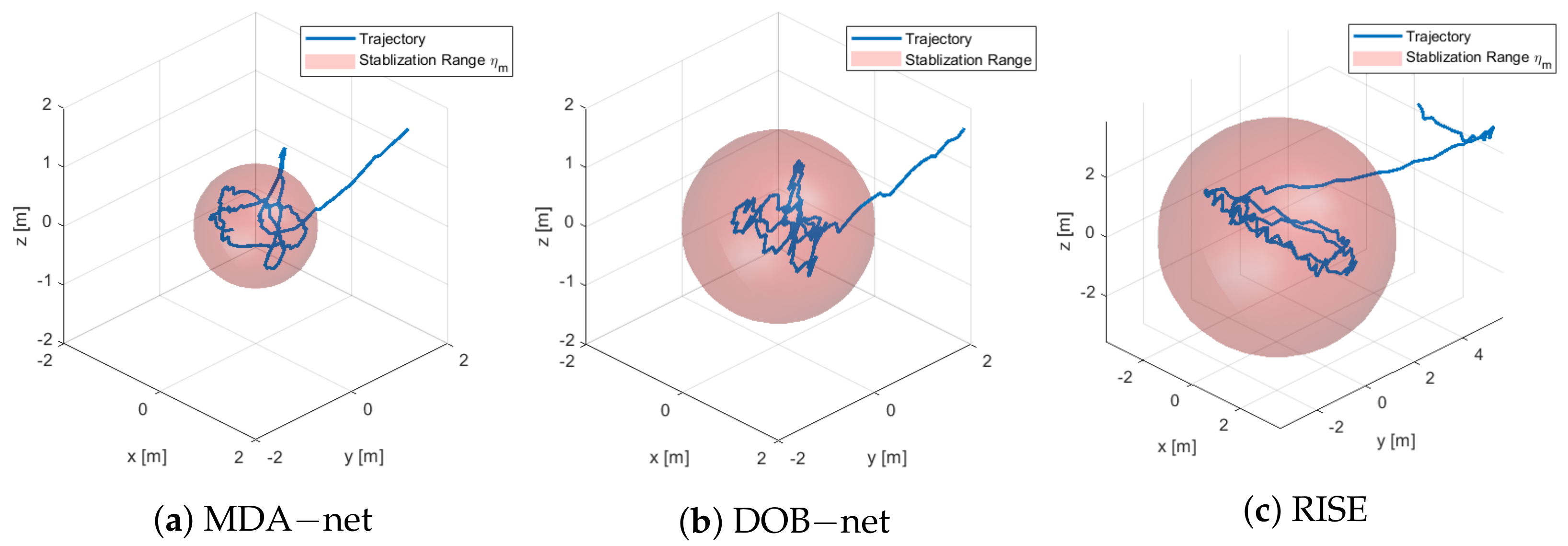
6.4. Stabilization Performance

In training and testing the controller network, the frequencies, amplitudes, and phrases of the disturbances are all randomly generated. This section compares the performances of DOB–net and the proposed MDA–net in solving Problem 1. The training score of the DOB–net is averaged over episodes and is about −713.3, and the averaged score of the MDA–net is about −455.6. Both scores are calculated according to Equation (2). The difference in training scores has shown that the MDA–net outperforms the DOB–net in dealing with the Markovian-jump disturbances simulated in this paper. As reported in [22], when dealing with disturbances whose characteristics do not change in an episode, the training score of the DOB–net could reach about −200.

Since the goal of the platform stabilization is to reach a minimum stabilization range, the regulation error is defined as the distance between the AUV platform to the targeted position (assumed the origin in the inertial space), given as

$$\eta =\parallel q\parallel .$$

(28)

Then the stabilization range is defined as the largest error after 5 seconds in an episode, as follows,

$${\eta }_m=\underset{5<t}{max}{\eta }_t.$$

(29)

Two trajectory examples are illustrated in Figure 6a and Figure 6b, respectively. In the first example, the disturbance amplitude exceeds the control saturation by 10 percent, while in the second example, the disturbance amplitudes are 80 percent of the control saturation. In both cases, the changes in the disturbances were given by Equation (26). The transparent spheres in blue and the ones in red indicate the stabilization ranges obtained by the MDA–net and the DOB–net, respectively. Both examples show that the proposed MDA–net has a smaller stabilization range than the DOB–net [22] in rejecting excessive disturbances subject to abrupt changes. The trajectories obtained from RISE were not shown for a clear illustration; the obtained stabilization ranges were often quite large. The smaller range indicates less challenge for the onboard manipulators, which is not discussed in this paper. The limitations of these numerical simulations are discussed in the last section.

We have also conducted extensive comparisons between MDA–net, DOB–net, and RISE in two different groups of scenarios. The amplitudes of the simulated disturbances in Group #1 could exceed the control saturation levels by 10%, while the amplitudes of the simulated disturbances in Group #2 could exceed the control saturation levels by 30% RISE controller [46]. In Figure 7a and Figure 7b, the results have shown that the MDA–net outperformed DOB–net and RISE in the test cases.

MDA–net was also tested in a tank, where the water flow was generated by a propeller fixed on the edge of the tank, as shown in Figure 8a. The direction of this propeller can be manually adjusted to create various disturbances. In the experiments, the sudden external impact was from the sudden changes in the disturbance generated by the position-fixed propeller. Its direction oscillated through manual control. The strength of the propeller force was adjusted as follows. By connecting the AUV to the frame fixed on the tank via a force-torque sensor, the forces acted on the AUV by disturbances were measured. The PWM signals to the propeller motor were adjusted such that the external forces acting on the AUV reached in [20, 40] N.

The saturation of the control inputs was confined to 30 N by setting the maximum value of the PWM signals of AUV thrusters. The AUV mass was about 14.5 kg. When testing the controller, AUV was detached from the force-torque sensor. Therefore, an example of the disturbance generated by the position-fixed propeller is given in Figure 9. The sudden changes were simulated by changing the propeller force and direction abruptly.

An underwater positioning system was implemented with 12 cameras that emit blue lights, as illustrated in Figure 8a. The AUV has four highly reflective markers on top Figure 8b. In addition, due to the low visibility underwater, the reflective markers are 30 mm wide. The positioning system was calibrated with an L-shaped bar with markers of known body coordinates. The cameras capture the markers and outputs pose estimates at 60 Hz.

The AUV system was built on BlueRov2 from Blue Robotics, Inc., Torrance, CA, USA as shown in Figure 8b. BlueRov2 is equipped with six thrusters and can translate in three directions, roll, and yaw. BlueRov2 communicates with a desktop and receives thruster commands at 50 Hz. The desktop also receives the pose estimates from the positioning system. In this AUV testbed, the desktop implements the DMA-net, making the BlueRov2 an AUV. The limitation of this setup is discussed in Section 7.

The obtained AUV trajectories are shown in Figure 10. The three approaches, MDA–net, DOB–net, and the RISE controller, were compared. The regulation errors and stabilization ranges of which are also shown in Figure 11. The limitation of the localization system in the lab tank will be discussed in Section 7.

One example of these experimental tests was shown in Figure 10; the AUVs started from the position around ${[1.1,1.8,1.2]}^T$. Three trajectories were separately obtained by three approaches, and they are shown in Figure 10a, Figure 10b, and Figure 10c, respectively. The trajectories have demonstrated that the MDA–net approach can offer better performance with a smaller stabilization range, while RISE can hardly keep the AUV near the origin.

7. Discussion and Future Work

The training of the controller does involve a lot of computational loads. When the trained controller is used online, at each time step, the computational cost is $O\left(n_n{n}_l\right)$, where $n_n$ is the number of neurons in each layer and $n_l$ is the number of layers, while the RISE approach is about $O\left(1\right)$. As observed, the evaluations of a trained controller network on a low-voltage CPU can achieve 100 Hz, which is sufficient for online applications.

Since the existence of the transform module, it is difficult to interpret the learned representation of the QP problem. It is, therefore, hard to analyze the stability of the system. In the future, additional regulations from Lyapunov’s theories should be imposed on the learning of controller networks.

While using disturbance knowledge in training might be avoided by closing the supervision from the aggregation of the platform model simulator and regularization on the simulator outputs, the platform model is also a module in the network, which could be extracted from GRU #1.

In addition, the abrupt changes in disturbances are naively made, and they may not reflect actual field situations. Future work includes testing the proposed approach in more realistic underwater environments. In addition, future improvements include orthogonal learning for different environments since MJLS and the sensitivity analysis have already provided a framework to extract principle components when a deep network is employed.

The limitation of the tank tests arises from the positioning approach since, in the real world, an auxiliary camera system is not available, and the sonar positioning system is often too noisy and has low bandwidth. In the future, an onboard underwater multi-band sonar sensor, camera, and localization system will be investigated.

The laptop receives the pose estimation from the motion capture system, implements the proposed RL approach, and sends the control signals to the ROV. The whole system is referred to as the testbed of the “AUV”. The testbed is not equivalent to AUV systems since the cameras are mounted along tank edges. However, the testbed may be sufficient to test the proposed control algorithm. We are developing an underwater sonar SLAM system to provide online state estimation to make the underwater fully autonomous. In the future, the sonar-based localization approach and the proposed transfer RL algorithm will be implemented in the updated hardware of the ROV, making it a real AUV.

8. Conclusions

This paper proposes an RL approach, referred to as MDA–net, for stabilizing a free-floating platform subject to excessive harmonic disturbances and control saturation. Through modeling the disturbed AUV platform as an MJLS, the harmonic model is integrated into the network for effective learning of the observer of the MJLS parameters. Sensitivity analysis of the optimal control problems is used to guide the learning of the controller network. Preliminary results from numerical simulations and tank tests have shown that MDA–net outperforms DOB–net when the disturbances have abrupt changes.

References

1. Griffiths, G. Technology and Applications of Autonomous Underwater Vehicles; CRC Press: Boca Raton, FL, USA, 2002; Volume 2. [Google Scholar]
2. Woolfrey, J.; Lu, W.; Liu, D. A Control Method for Joint Torque Minimization of Redundant Manipulators Handling Large External Forces. J. Intell. Robot. Syst. 2019, 96, 3–16. [Google Scholar] [CrossRef] [Green Version]
3. Xie, L.L.; Guo, L. How much uncertainty can be dealt with by feedback? IEEE Trans. Autom. Control 2000, 45, 2203–2217. [Google Scholar]
4. Gao, Z. On the centrality of disturbance rejection in automatic control. ISA Trans. 2014, 53, 850–857. [Google Scholar] [CrossRef] [PubMed] [Green Version]
5. Li, S.; Yang, J.; Chen, W.H.; Chen, X. Disturbance Observer-Based Control: Methods and Applications; CRC Press: Boca Raton, FL, USA, 2014. [Google Scholar]
6. Skogestad, S.; Postlethwaite, I. Multivariable Feedback Control: Analysis and Design; Wiley: New York, NY, USA, 2007; Volume 2. [Google Scholar]
7. Doyle, J.C.; Glover, K.; Khargonekar, P.P.; Francis, B.A. State-space solutions to standard H/sub 2/and H/sub infinity/control problems. IEEE Trans. Autom. Control 1989, 34, 831–847. [Google Scholar] [CrossRef]
8. Åström, K.J.; Wittenmark, B. Adaptive Control; Courier Corporation: Washington, DC, USA, 2013. [Google Scholar]
9. Lu, W.; Liu, D. Active task design in adaptive control of redundant robotic systems. In Proceedings of the Australasian Conference on Robotics and Automation (ARAA 2017), Sydney, Australia, 11–13 December 2017. [Google Scholar]
10. Lu, W.; Liu, D. A frequency-limited adaptive controller for underwater vehicle-manipulator systems under large wave disturbances. In Proceedings of the World Congress on Intelligent Control and Automation, Changsha China, 4–8 July 2018. [Google Scholar]
11. Salgado-Jimenez, T.; Spiewak, J.M.; Fraisse, P.; Jouvencel, B. A robust control algorithm for AUV: Based on a high order sliding mode. In Proceedings of the OCEANS’04 MTTS/IEEE TECHNO-OCEAN’04, Kobe, Japan, 9–12 November 2004; Volume 1, pp. 276–281. [Google Scholar]
12. Chen, W.H.; Ballance, D.J.; Gawthrop, P.J.; O’Reilly, J. A nonlinear disturbance observer for robotic manipulators. IEEE Trans. Ind. Electron. 2000, 47, 932–938. [Google Scholar] [CrossRef] [Green Version]
13. Chen, W.H.; Ballance, D.J.; Gawthrop, P.J.; Gribble, J.J.; O’Reilly, J. Nonlinear PID predictive controller. IEE Proc.-Control Theory Appl. 1999, 146, 603–611. [Google Scholar] [CrossRef] [Green Version]
14. Kim, K.S.; Rew, K.H.; Kim, S. Disturbance observer for estimating higher order disturbances in time series expansion. IEEE Trans. Autom. Control 2010, 55, 1905–1911. [Google Scholar]
15. Su, J.; Chen, W.H.; Li, B. High order disturbance observer design for linear and nonlinear systems. In Proceedings of the 2015 IEEE International Conference on Information and Automation, Beijing, China, 2–5 August 2015; pp. 1893–1898. [Google Scholar]
16. Johnson, C. Optimal control of the linear regulator with constant disturbances. IEEE Trans. Autom. Control 1968, 13, 416–421. [Google Scholar] [CrossRef]
17. Johnson, C. Accomodation of external disturbances in linear regulator and servomechanism problems. IEEE Trans. Autom. Control 1971, 16, 635–644. [Google Scholar] [CrossRef]
18. Chen, W.H.; Yang, J.; Guo, L.; Li, S. Disturbance-observer-based control and related methods—An overview. IEEE Trans. Ind. Electron. 2015, 63, 1083–1095. [Google Scholar] [CrossRef] [Green Version]
19. Li, S.; Sun, H.; Yang, J.; Yu, X. Continuous finite-time output regulation for disturbed systems under mismatching condition. IEEE Trans. Autom. Control 2014, 60, 277–282. [Google Scholar] [CrossRef]
20. Gao, H.; Cai, Y. Nonlinear disturbance observer-based model predictive control for a generic hypersonic vehicle. Proc. Inst. Mech. Eng. Part I J. Syst. Control Eng. 2016, 230, 3–12. [Google Scholar] [CrossRef]
21. Ghafarirad, H.; Rezaei, S.M.; Zareinejad, M.; Sarhan, A.A. Disturbance rejection-based robust control for micropositioning of piezoelectric actuators. Comptes Rendus Mécanique 2014, 342, 32–45. [Google Scholar] [CrossRef]
22. Wang, T.; Lu, W.; Yan, Z.; Liu, D. DOB–net: Actively rejecting unknown excessive time-varying disturbances. In Proceedings of the 2020 IEEE International Conference on Robotics and Automation (ICRA), Paris, France, 31 May–31 August 2020; pp. 1881–1887. [Google Scholar]
23. Camacho, E.F.; Alba, C.B. Model Predictive Control; Springer Science & Business Media: Berlin, Germany, 2013. [Google Scholar]
24. Maeder, U.; Morari, M. Offset-free reference tracking with model predictive control. Automatica 2010, 46, 1469–1476. [Google Scholar] [CrossRef]
25. Yang, J.; Zheng, W.X.; Li, S.; Wu, B.; Cheng, M. Design of a prediction-accuracy-enhanced continuous-time MPC for disturbed systems via a disturbance observer. IEEE Trans. Ind. Electron. 2015, 62, 5807–5816. [Google Scholar] [CrossRef]
26. Sutton, R.S.; Barto, A.G. Reinforcement Learning: An Introduction; MIT Press: Cambridge, MA, USA, 2018. [Google Scholar]
27. Sæmundsson, S.; Hofmann, K.; Deisenroth, M.P. Meta reinforcement learning with latent variable gaussian processes. arXiv 2018, arXiv:1803.07551. [Google Scholar]
28. Kormushev, P.; Caldwell, D.G. Improving the energy efficiency of autonomous underwater vehicles by learning to model disturbances. In Proceedings of the 2013 IEEE/RSJ International Conference on Intelligent Robots and Systems, Tokyo, Japan, 3–7 November 2013; pp. 3885–3892. [Google Scholar]
29. Sun, H.; Li, Y.; Zong, G.; Hou, L. Disturbance attenuation and rejection for stochastic Markovian jump system with partially known transition probabilities. Automatica 2018, 89, 349–357. [Google Scholar] [CrossRef]
30. Yao, X.; Park, J.H.; Wu, L.; Guo, L. Disturbance-observer-based composite hierarchical antidisturbance control for singular Markovian jump systems. IEEE Trans. Autom. Control 2018, 64, 2875–2882. [Google Scholar] [CrossRef]
31. Zhang, L.; Boukas, E.K. Stability and stabilization of Markovian jump linear systems with partly unknown transition probabilities. Automatica 2009, 45, 463–468. [Google Scholar] [CrossRef]
32. Zhang, J.; Shi, P.; Lin, W. Extended sliding mode observer based control for Markovian jump linear systems with disturbances. Automatica 2016, 70, 140–147. [Google Scholar] [CrossRef]
33. Rahman, S.; Li, A.Q.; Rekleitis, I. Svin2: An underwater slam system using sonar, visual, inertial, and depth sensor. In Proceedings of the 2019 IEEE/RSJ International Conference on Intelligent Robots and Systems (IROS), Macau, China, 3–8 November 2019; pp. 1861–1868. [Google Scholar]
34. Antonelli, G. Underwater Robots; Springer: Cham, Switzerland, 2014; Volume 3. [Google Scholar]
35. Nagabandi, A.; Kahn, G.; Fearing, R.S.; Levine, S. Neural network dynamics for model-based deep reinforcement learning with model-free fine-tuning. In Proceedings of the 2018 IEEE International Conference on Robotics and Automation (ICRA), Brisbane, QLD, Australia, 21–25 May 2018; pp. 7579–7586. [Google Scholar]
36. Sandholm, T.W.; Crites, R.H. Multiagent reinforcement learning in the iterated prisoner’s dilemma. Biosystems 1996, 37, 147–166. [Google Scholar] [CrossRef] [PubMed]
37. Wang, T.; Lu, W.; Liu, D. Excessive Disturbance Rejection Control of Autonomous Underwater Vehicle using Reinforcement Learning. In Proceedings of the Australasian Conference on Robotics and Automation 2018, Lincoln, New Zealand, 4–6 December 2018. [Google Scholar]
38. van der Himst, O.; Lanillos, P. Deep Active Inference for Partially Observable MDPs. arXiv 2020, arXiv:2009.03622. [Google Scholar]
39. Hausknecht, M.; Stone, P. On-policy vs. off-policy updates for deep reinforcement learning. In Proceedings of the Deep Reinforcement Learning: Frontiers and Challenges, IJCAI 2016 Workshop, New York, NY, USA, 9–11 July 2016. [Google Scholar]
40. Oh, J.; Chockalingam, V.; Singh, S.; Lee, H. Control of memory, active perception, and action in minecraft. arXiv 2016, arXiv:1605.09128. [Google Scholar]
41. Yao, X.; Guo, L. Composite anti-disturbance control for Markovian jump nonlinear systems via disturbance observer. Automatica 2013, 49, 2538–2545. [Google Scholar] [CrossRef]
42. Gill, P.E.; Murray, W.; Saunders, M.A. SNOPT: An SQP algorithm for large-scale constrained optimization. SIAM Rev. 2005, 47, 99–131. [Google Scholar] [CrossRef]
43. Mnih, V.; Badia, A.P.; Mirza, M.; Graves, A.; Lillicrap, T.; Harley, T.; Silver, D.; Kavukcuoglu, K. Asynchronous methods for deep reinforcement learning. In Proceedings of the International Conference on Machine Learning, New York, NY, USA, 19–24 June 2016; pp. 1928–1937. [Google Scholar]
44. Bottou, L. Large-scale machine learning with stochastic gradient descent. In Proceedings of the COMPSTAT’2010, Paris, France, 22–27 August 2010; Physica-Verlag: Heidelberg, Germany, 2010; pp. 177–186. [Google Scholar]
45. Amos, B.; Jimenez, I.; Sacks, J.; Boots, B.; Kolter, J.Z. Differentiable MPC for end-to-end planning and control. In Proceedings of the 2018 Conference on Neural Information Processing Systems, Montreal, QC, Canada, 3–8 December 2018; pp. 8289–8300. [Google Scholar]
46. Fischer, N.; Kan, Z.; Kamalapurkar, R.; Dixon, W.E. Saturated RISE feedback control for a class of second-order nonlinear systems. IEEE Trans. Autom. Control 2013, 59, 1094–1099. [Google Scholar] [CrossRef] [Green Version]
Figure 1. Network architecture of DOB–net.
Jmse 11 00285 g001
Figure 2. Observer network.
Jmse 11 00285 g002
Figure 3. Network Architecture of MDA–net.
Jmse 11 00285 g003
Figure 4. Disturbance prediction example by MDA–net. Solid curves showing ground truth; marked curves showing 2.5 (s) prediction from three different instants.
Jmse 11 00285 g004
Figure 5. Disturbance prediction example by DOB–net. Solid curves showing ground truth; marked curves showing 2.5 (s) prediction from three different instants.
Jmse 11 00285 g005
Figure 6. Examples of the trajectories obtained by MDA–net and DOB–net, respectively. (a) The stabilization range etam obtained from MDA–net is 0.43 (m) and etam obtained from DOB–net is 0.54 (m); (b) The stabilization range etam obtained from MDA–net is 0.22 (m), and etam obtained from DOB–net is 0.45 (m).
Jmse 11 00285 g006
Figure 7. Comparison among MDA–net, DOB–net, and RISE under disturbances in Groups #1 and #2.
Jmse 11 00285 g007
Figure 8. Testbed description: tank, wave generator, positioning system, and AUV with markers.
Jmse 11 00285 g008
Figure 9. The forces in the x− and y−directions are shown in red and green, respectively. The disturbance in the z− direction (shown in blue) is negligible.
Jmse 11 00285 g009
Figure 10. An example of trajectory and position regulation errors from tank tests. The blue curves represent the trajectories from three approaches, and the transparent spheres present stabilization ranges ηm defined in Equation (29).
Jmse 11 00285 g010
Figure 11. Regulation errors η (solid curves) and stabilization ranges ηm (dashed lines) obtained from MDA–net (in red), DOB–net (in green), and RISE (in blue), respectively.
Jmse 11 00285 g011