Water Temperature Prediction Using Improved Deep Learning Methods through Reptile Search Algorithm and Weighted Mean of Vectors Optimizer

Abstract

Precise estimation of water temperature plays a key role in environmental impact assessment, aquatic ecosystems’ management and water resources planning and management. In the current study, convolutional neural networks (CNN) and long short-term memory (LSTM) network-based deep learning models were examined to estimate daily water temperatures of the Bailong River in China. Two novel optimization algorithms, namely the reptile search algorithm (RSA) and weighted mean of vectors optimizer (INFO), were integrated with both deep learning models to enhance their prediction performance. To evaluate the prediction accuracy of the implemented models, four statistical indicators, i.e., the root mean square errors (RMSE), mean absolute errors, determination coefficient and Nash–Sutcliffe efficiency were utilized on the basis of different input combinations involving air temperature, streamflow, precipitation, sediment flows and day of the year (DOY) parameters. It was found that the LSTM-INFO model with DOY input outperformed the other competing models by considerably reducing the errors of RMSE and MAE in predicting daily water temperature.

1. Introduction

Water temperature is a fundamental aspect impacting the quality of aquatic environments [1]. Increasing water temperature can boost chemical and biological processes that lead to different problems. For instance, when water temperature increases, dissolved oxygen reduces, and aquatic plants and pertinent aqua-systems are threatened [2,3]. In addition, it can affect the ice formation or evaporation rate [4,5]. Water temperature is also vital in assessing climate change in hydrological projects such as considering thermal dynamics during the construction of hydraulic structures such as dams [6,7,8]. As a result, developing a precise method to predict water temperature seems necessary to protect and manage aqua-systems.

Over the course of the past decades, several methodologies, such as mathematical models [9], stochastic methods [10], probabilistic techniques [11], statistical approaches [12], and remote sensing techniques [13], have been presented for predicting water temperature. More recently, machine learning (ML) methods have been successfully applied to model/predict water temperature [14].

In this sense, some studies expanded convectional ML models for modeling environmental problems such as water temperature [15,16,17,18,19,20]. For instance, three ML models were developed: a feed-forward neural network, a decision tree, and Gaussian process regression for estimating water temperature. The input vector of the developed model was air temperature, discharge, and time element (day of year) obtained from eight river stations. The models were evaluated by comparing the outcomes with the ones of aire2stream model, which is a hybrid model combining physical-based and stochastic calibration methods. In most cases, the results of the aire2stream model were superior to other proposed models based on several statistical indices. Moreover, the decision tree outperformed the other ML models, followed by the feed-forward neural network and Gaussian process regression models [21]. In another research, a convolutional neural network (CNN) was implemented to estimate the monthly subsurface water temperature in the Pacific Ocean. Input data consisted of sea surface height, sea surface temperature, and sea surface salinity measured with satellite remote sensors. In addition, the Argo data were used to validate the model’s results. The model enhanced the estimation and indicated promising outcomes for the satellite observation [22]. In a more recent study, the extended long short-term memory neural network (LSTM) capability was examined for predicting daily river temperature [19]. The data were collected from nine gauges in different rivers across the world. The proposed model demonstrated an accurate result in mapping water temperature even in the Yangtze River, the water temperature of which is induced by the operation gate.

Over the course of the past ten years, there has been a debate on the improvement of regular (single) ML models embedded with novel optimization strategies [23,24,25]. Subsequently, the accuracy of the ML models can be improved by integrating them with other soft computing approaches (e.g., heuristic algorithms) or optimization methods (such as swarm intelligence). In this sense, a back propagation neural network (BP) model was introduced and optimized through the particle swarm optimization algorithm (PSO) for predicting water temperature in the Yangtze River [26]. Three models were categorized by different input data, including BPPSO1 (air temperature as input), BPPSO2 (air temperature and discharge as input), and BPPSO3 (air temperature, discharge, and day of the year as input). The results showed that considering more input variables would lead to better prediction and help to model river thermal dynamic behavior more accurately. An LSTM model was established and optimized with a genetic algorithm (GA) for water temperature prediction to assess urban rivers’ water quality [27]. The hourly water temperatures for five years were considered as an input vector. The performance of the proposed model was compared with a recurrent neural network model. In conclusion, the GA-LSTM was introduced as an authentic deep machine learning technique for time-series predictions.

Among different nature-based optimization methods, the reptile search algorithm (RSA) is an innovative optimization algorithm proposed by Abualigah et al. [28]. The present technique is motivated by the hunting performance of reptiles and it is divided into two walking and hunting categories. Two mathematical models were proposed to update the position of crocodiles based on diverse and optimal search areas. The accuracy of this model was proven with seven real-world engineering criteria, twenty-three classical, thirty CEC2017, and ten CEC2019 test functions. The results were compared with ten optimization algorithms and showed the model’s superiority over other models. Several studies have been successfully developed based on RSA since then [29,30,31].

Recently, an optimization algorithm relying on the weighted mean of vectors (INFO) was presented. This model applies convergence acceleration and mean-base law to update the position of the vectors. Next, the updated vectors are combined to establish a possible solution. Then, local search is extended to enhance exploitation and ignore low-precise solutions. In their study, the developed model was evaluated with five constrained engineering test cases and forty-eight mathematical test functions. The results were also compared with five optimization algorithms and nine advanced algorithms. Moreover, the ability to use this algorithm in real engineering problems was verified by four complicated, challenging, and constrained issues. The findings indicated that the model is highly efficient in optimizing complex phenomena with unacknowledged search areas [32]. The INFO algorithm has been applied to estimate the solar cell parameters. The model was compared with seven optimization algorithms, including tunicate swarm algorithm, chimp optimization algorithm, moth–flame optimizer, Harris hawk optimization, grey wolf optimization, sine cosine algorithm, along with the Runge–Kutta optimization, and showed a higher performance [33].

The primary purposes of this study are fourfold: (1) to evaluate the individual machine learning models, including LSTM and CNN for modeling river water temperature; (2) to assess two recently introduced optimization algorithms for improving the accuracy of individual deep learning models; (3) to analyze the impact of each input variable including T_a (air temperature), Q (discharge), P (precipitation), S (sediment load) and time element (day of the year) on achieving high accuracy; and (4) to compare the performance of the proposed model with observed data, using various statistical approaches. To the best of our knowledge, the optimization of the LSTM and CNN models through the application of RSA and INFO algorithms has not been studied in water temperature prediction, which demonstrates the contribution of this research.

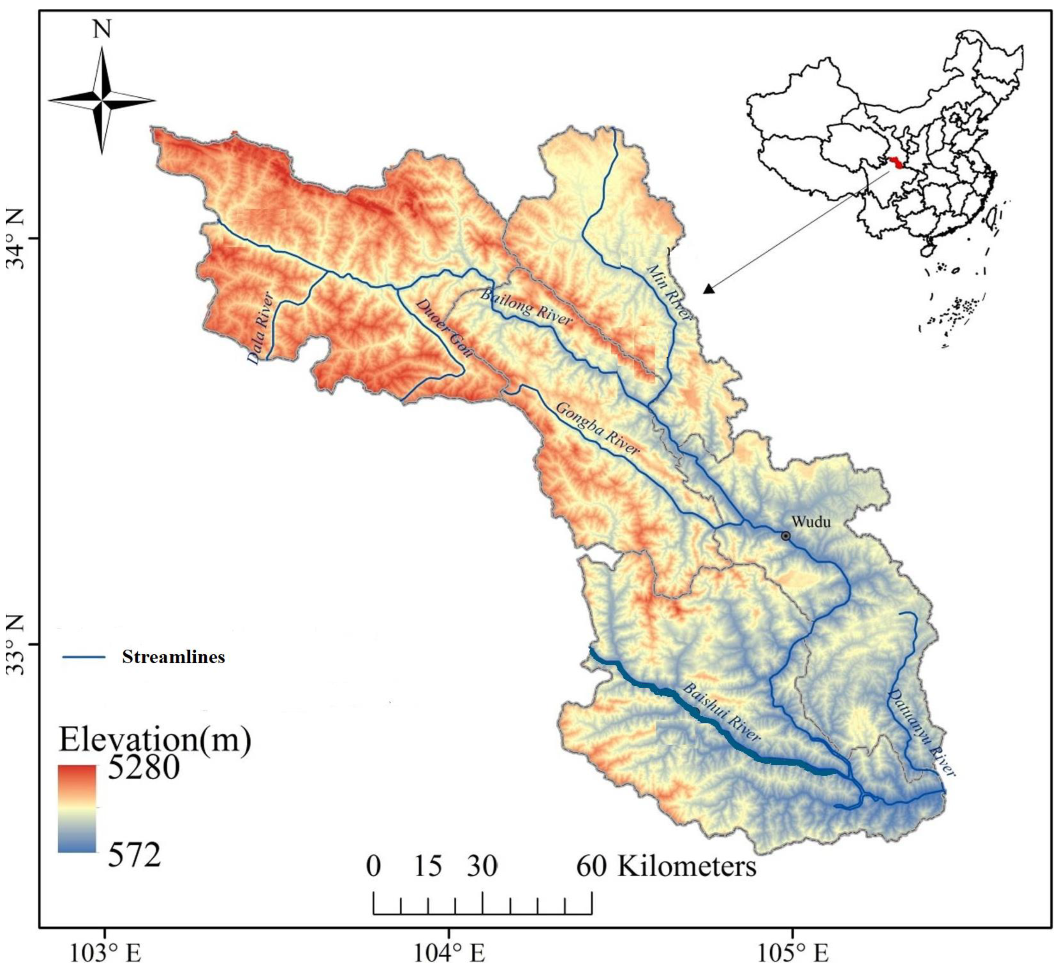
2. Case Study

Bailong River Basin is selected in this study as a case study area (Figure 1). Bailong River is a secondary tributary of the Yangtze River, while simultaneously being the main largest tributary of the Jialing River. Bailong Basin is located in north–central China, in the 32°36′–34°24′ N longitude and 103°00′–105°30′ E latitude coordinates. The basin covers a catchment area of 17,845 Km² and the river spread is of 452 Km. The elevation of the Bailong River basin is higher in the northwest and lower in the southeast, varying from 520 to 4358 m. Rainfall is the main source of the Bailong River flow. The mean annual rainfall in the basin ranges from 520 mm to 910 mm, whereas the average annual temperature varies from 6.1 to 14.9 °C. A big portion of the yearly rainfall, i.e., 60% to 80%, occurs from June to September in the form of heavy rainfall events. Wudu hydroclimatic station is adopted in this study to model the water temperature of the Basin. The Wudu station is situated around 33°23′ N longitude and 104°55′ E latitude coordinates. Daily streamflow, water temperature, precipitation, and sediment data were collected from the yearly hydrological books, whereas the daily air temperature data were obtained from the China Meteorological Administration (CMA) department for the period from 2007 to 2012. Different input combinations of air temperature, streamflow, precipitation, and sediment flows were adopted to model the water temperature of the basin. In addition to these inputs, day of the year (DOY) input was also added to see the effect of this input on the prediction accuracy of water temperature modeling. For better representation of data, cross-validation techniques were applied. A total of six years’ worth of datasets were divided into three equals (two years) sub-datasets, i.e., from M1 to M3. Each time, one sub-dataset was adopted as a test dataset, whereas the remaining four years’ data were used as a training dataset. The statistical overview of the dataset is depicted in

Table 1. The statistical overview of dataset.

	Mean	Min.	Max	Skewness	Std. Dev.
Air Temperature
M1	15.41	−4	28.9	−0.282	8.165
M2	15.41	−2.3	31.9	−0.145	7.942
M3	14.82	−2.1	30.2	−0.179	8.314
Sediment Flow
M1	207.8	0.001	4330	5.117	484.3
M2	128.4	1.88	8710	10.55	487.4
M3	231.0	1.9	8640	6.770	687.3
Streamflow
M1	108.3	38.3	327	1.047	56.29
M2	102.4	33.8	413	1.217	59.3
M3	128.4	36	653	1.642	92.17
Precipitation
M1	1.257	0	31.3	4.413	3.548
M2	1.10	0	42	5.360	3.503
M3	1.270	0	34	4.799	3.907
Water Temperature
M1	11.98	1.2	21	−0.265	5.477
M2	12.33	1.8	22.8	−0.142	5.300
M3	12.35	2.2	28.8	−0.245	5.079

.

3. Methods

In this study, the performances of two deep learning models optimized using two recently introduced optimization algorithms were compared in predicting daily water temperature time series. A basic description of both deep learning methods and optimization algorithms is provided below.

3.1. Deep Learning Based Models

3.1.1. Convolution Neural Network (CNN)

The convolution neural network model is widely used around the globe in many areas of research and it is also known as ConvNet. It is a type of artificial neural network (ANN) with the ability to feed forward. CNN has a finite number of layers, which establish many properties of input data with multiple levels of abstraction. Initially, in 1959, David Hubel and Torsten Wiesel determined that the neurons of a cat’s brain form in the layers. These are developed to identify visual patterns by, first, extracting the local structures, and then combining the extracted structures for advanced-level depiction. After this development, this became a vital principle for deep learning. Later on, David Hubel and Torsten Wiesel applied this technique to monkeys to established extracellular components from sole elements and to stimulate the retinas with spots. They also published their papers, entitled “Receptive fields of single neurons in cat’s striate cortex” [34] and “Receptive fields and functional architecture of monkey striate cortex” [35]. After this, Fukushima [36] developed recognition, which has multiple layers with a self-organizing neural network and a capacity of finding visual patterns. This construction is the first model of CNN. The conceptual model of CNN is described below in Figure 2.

Input Layer: The major purpose of this layer is to feed the inputs to the convolution layer.

Convolution Layer: This layer is the most vital part in the structure of CNN, as it consists of the convolution kernels which help to convert loaded inputs to generate an output. It extracts the features from the input data and uses them for further processing in CNN. This layer is important for two major reasons: sparse connection and weight sharing. In the first part, a small number of weights is provided to connect two layers. On the other hand, in the neural network, it is required that each neuron of one layer connect with each neuron of the other layer. Therefore, in CNN, the amount of memory stored in these weights is also small, which makes this model memory-efficient. Secondly, in weight sharing, as all weights work with every input, it takes one set of weights for all inputs—this process reduces the training time and cost.

Pooling Layer: This layer uses a bigger part of the feature map and shrinks that to a lower-size feature map. In each pool, it keeps all the important features of the previous convolution layer. There are many practices for pooling, such as max pooling, average pooling, min pooling, tree pooling, and gated pooling.

Fully Connected Layer: In this fully connected layer, all neurons are mapped with all neurons from their past layers. This is the last stage of each convolutional neural network, utilized as a regression. It is a combination of two laws, firstly as feed-forward ANN, and secondly as MLP (multilayer perceptron neural network).

Activation Functions: The activation function is used to make an association between input and output; it also instructs the neuron on when to fire or not. Here, in the CNN model, a non-linear activation layer is used, which helps to manage the mapping nonlinearly between inputs to outputs. In the training session of the model, it is used to reduce errors while using the backpropagation method.

Sigmoid function: This sigmoid function has the real input and fixes the output in the range of [0, 1]. The sigmoid function’s curve is ‘S’-shaped and it is shown mathematically as:

$$f{\left(x\right)}_{sigm}=\frac{1}{1+e^{-x}}$$

(1)

Tanh: This activation function is utilized to fix the input values in [−1, 1]; mathematically, it is represented as:

$$f{\left(x\right)}_{\tanh }=\frac{e^x-e^{-x}}{e^x+e^{-x}}$$

(2)

ReLU: In CNN, this rectifier linear unit (ReLU) [37] is widely used as an activation function. It translates every input value to a positive number with a nominal computation load. It is mathematically described as:

$$f{\left(x\right)}_{\mathrm{Re}LU}=Max\left(0,x\right)$$

(3)

3.1.2. Long Short Term Memory (LSTM)

The long short-term memory network (LSTM) model is very applicable in different areas of research and is developed based on the error flow of recurrent neural networks (RNN). Its major contribution is the use of temporal information for the input to the model; this makes the LSTM model unique compared to the other machine learning models. This developed LSTM model contains the memory cell, which has a particular neuron structure. The LSTM model also has the expertise to supply the information at a random time. The input gate, output gate, and forget gate are the three main gates of the neuron’s memory cell. In addition, each gate has the same input neuron, and each gate also has its activation function. Long delays are inaccessible to existing structures because the back-propagated mistake either explodes or rots dramatically. These squares can be considered an idea for a differentiable form of the memory that contributes to an advanced PC. This contribution to the cells is increased by the initiation of the information input, the output is duplicated by that of the yielding door, and the past cell esteems are increased by the fail-to-remember entryway [38,39,40,41]. Here, the cells and gates are further collaborating with the net. The LSTM model’s flow chart is shown in Figure 3.

3.2. Optimization Algorithms

3.2.1. Weighted Mean of Vectors (INFO) Optimizer

In the area of population-based modeling, the weighted mean of vectors (INFO) optimizer is a popular optimization model and known for its accuracy in the model output. The weighted mean is calculated from input vectors that have the possible solution set in the search space. The average of the positions evaluated is built upon the weights of every vector. The large weighted positions of the set of vectors play a leading role in the calculations of the weighted mean. The weighting of the positions helps to find out the outcome of the solutions on the weighted mean. This algorithm provides the optimal solution over many consecutive generations. In every generation, three operators help in updating the position of the vector, as discussed below in the stages of position update [32].

Stage 1 (Updating Rule): The first step in the INFO model is the updating rule, which enhances the population diversity in the search practice. This updating rule operator’s job is to utilize the weighted mean of the vector to construct new vectors. It has two major roles in the development of the INFO model: The first is the mean-based rule, which is obtained from the weighted mean (WM) for a set of random vectors. The second role is convergence acceleration (CA), which is used to escalate the convergence speed and performance of the model to get an optimal solution.

Let the model have the population of Np vectors in D dimensional search domain ($X_{l,j}^g=\left\{X_{l,1}^g,X_{l,2}^g,X_{l,3}^g,\dots \dots ,X_{l,D}^g\right\}, l=1,2,3,\dots ,Np$). In the initial step, controlling parameters are introduced, $\sigma$ is the weighted mean factor, $\beta$ is the change according to the exponential function, the maximum number of generations is defined by $Max g$ and $\delta$ is the scaling factor.

$$\begin{array}{l}\delta =2\beta \times rand-\beta \\ \beta =2\exp \left(-4\times \frac{g}{Max g}\right)\end{array}$$

(4)

The mean-based rule which leads to the mean rule is defined below in Equation (5).

$$MeanRule=r\times WM{1}_l^g+\left(1-r\right)\times WM{2}_l^g, l=1,2,3,\dots ,Np$$

(5)

$$WM{1}_l^g=\delta \times \frac{w_1\left(x_{a1}-x_{a2}\right)+w_2\left(x_{a1}-x_{a3}\right)+w_3\left(x_{a2}-x_{a3}\right)}{w_1+w_2+w_3+\epsilon }+\epsilon \times rand, l=1,2,3,\dots ,Np$$

(5a)

$$w_1=\cos \left(\left(f\left(x_{a1}\right)-f\left(x_{a2}\right)\right)+\pi \right)\times \exp \left(-\left|\frac{f\left(x_{a1}\right)-f\left(x_{a2}\right)}{\omega }\right|\right)$$

(5b)

$$w_2=\cos \left(\left(f\left(x_{a1}\right)-f\left(x_{a3}\right)\right)+\pi \right)\times \exp \left(-\left|\frac{f\left(x_{a1}\right)-f\left(x_{a3}\right)}{\omega }\right|\right)$$

(5c)

$$w_3=\cos \left(\left(f\left(x_{a2}\right)-f\left(x_{a3}\right)\right)+\pi \right)\times \exp \left(-\left|\frac{f\left(x_{a2}\right)-f\left(x_{a3}\right)}{\omega }\right|\right)$$

(5d)

$$\omega =\max \left(f\left(x_{a1}\right),f\left(x_{a2}\right),f\left(x_{a3}\right)\right)$$

(5e)

In the above equations, the wavelet function is implemented for combining the translations and dilations of the selected mother wavelet, which helps to generate effective fluctuations for evaluating the vector’s weight. Equation (5a), depicts the general calculations of the weighted mean for the three vectors $\left(x_{a1},x_{a2},x_{a3}\right)$ given in Equations (5b)–(5d), respectively. $f\left(x_{a1}\right),f\left(x_{a2}\right),f\left(x_{a3}\right)$ are the fitness functions and $w_1,w_2,w_3$ are the weight functions of the vectors.

$$WM{2}_l^g=\delta \times \frac{w_1\left(x_{bs}-x_{bt}\right)+w_2\left(x_{bs}-x_{ws}\right)+w_3\left(x_{bt}-x_{ws}\right)}{w_1,w_2,w_3+\epsilon }+\epsilon \times rand, l=1,2,3,\dots ,Np$$

(6)

$$w_1=\cos \left(\left(f\left(x_{bs}\right)-f\left(x_{bt}\right)\right)+\pi \right)\times \exp \left(-\left|\frac{f\left(x_{bs}\right)-f\left(x_{bt}\right)}{\omega }\right|\right)$$

(6a)

$$w_2=\cos \left(\left(f\left(x_{bs}\right)-f\left(x_{ws}\right)\right)+\pi \right)\times \exp \left(-\left|\frac{f\left(x_{bs}\right)-f\left(x_{ws}\right)}{\omega }\right|\right)$$

(6b)

$$w_3=\cos \left(\left(f\left(x_{bt}\right)-f\left(x_{ws}\right)\right)+\pi \right)\times \exp \left(-\left|\frac{f\left(x_{bt}\right)-f\left(x_{ws}\right)}{\omega }\right|\right)$$

(6c)

$$\omega =f\left(x_{ws}\right)$$

(6d)

Here, $f\left(x\right)$ is considered an objective function and integers taken from [1, Np] as $a_1\ne a_2\ne a_3\ne l$. The solutions of gth generation which are taken as the best, better, and worse solutions are defined as $x_{bs},x_{bt},x_{ws}$, respectively. The weight functions are utilized to search the solution space globally for the INFO model with taken r as a random number in [0, 0.5].

Convergence acceleration (CA) is vital for the rule operator (stage 1), as it has utilized the best vector to move ahead as the current vector for global search. In this model, the best solution is the nearest solution to global optima. CA assists the vectors to move in the improved direction [42].

$$CA=rand n \times \frac{\left(x_{bs}-x_{a1}\right)}{\left(f\left(x_{bs}\right)-f\left(x_{a1}\right)+\epsilon \right)}$$

(7)

Here, a random number with normal distribution is denoted by rand n. In addition, the required new vector is obtained using Equation (8), as shown below.

$$z_l^g=x_l^g+\sigma \times MeanRule+CA$$

(8)

For the exploration phase, the model searches globally to discover the search domain. The following equations are used to update rule-based for $x_{bs},x_{bt},x_l^g,x_{a1}^g$.

$$\begin{array}{l}if rand<0.5\\ z{1}_l^g=x_l^g+\sigma \times MeanRule+rand n\times \frac{\left(x_{bs}-x_{a1}^g\right)}{\left(f\left(x_{bs}\right)-f\left(x_{a1}^g\right)+1\right)}\end{array}$$

(9)

$$z{2}_l^g=x_{bs}+\sigma \times MeanRule+rand n\times \frac{\left(x_{a1}^g-x_b^g\right)}{\left(f\left(x_{a1}^g\right)-f\left(x_b^g\right)+1\right)}$$

(10)

$$\begin{array}{l}else\\ z{1}_l^g=x_a^g+\sigma \times MeanRule+rand n\times \frac{\left(x_{a2}^g-x_{a3}^g\right)}{\left(f\left(x_{a2}^g\right)-f\left(x_{a3}^g\right)+1\right)}\end{array}$$

(11)

$$\begin{array}{l}z{2}_l^g=x_{bt}+\sigma \times MeanRule+rand n\times \frac{\left(x_{a1}^g-x_{a2}^g\right)}{\left(f\left(x_{a1}^g\right)-f\left(x_{a2}^g\right)+1\right)}\\ end\end{array}$$

(12)

Here, in the gth generation, the newly obtain vectors are $z{1}_l^g \& z{2}_l^g$, and the scaling rate of the vector is proposed as $\sigma$ and defined as given below in Equation (13). Moreover, Equation (14) depicts the change based on $\alpha$ in exponential function.

$$\sigma =2\alpha \times rand-\alpha$$

(13)

$$\alpha =c \exp \left(-d\times \frac{g}{Max g}\right)$$

(14)

Here, c = 2 and d = 4 are the constant numbers, the large value of the parameter $\sigma$ indicates that the current position of the vector deviates from WM (exploration phase), and the small value directed that the current position vector move toward the WM (exploitation phase).

Stage 2 (Vector Combining): Vector-combining is the second stage, which is responsible for enhancing the population diversity and improving the local search. $z{1}_l^g \& z{2}_l^g$ are combined with the rule operator’s vector $x_l^g$ for rand < 0.5 to generate a new vector $u_l^g$. This vector will ensure the improvement of the local search ability with the new and capable vector.

$$\begin{array}{l}If rand<0.5\\ u_l^g=z{1}_l^g+\mu \left|z{1}_l^g-z{2}_l^g\right|\end{array}$$

(15)

$$\begin{array}{l}else\\ u_l^g=z{2}_l^g+\mu \left|z{1}_l^g-z{2}_l^g\right|\\ end\end{array}$$

(16)

$$\begin{array}{l}else\\ u_l^g=x_l^g\\ end\end{array}$$

(17)

Here, vector-combining in gth generation $u_l^g$ is attained, $\mu =0.05\times rand n$.

Stage 3 (Local Search): The third step in the INFO model is local search; it helps to encourage exploitation and convergence to attain the global best. The global best position is denoted here as $x_{best}^g$ and the novel vector will be around this position.

$$\begin{array}{l}if rand<0.5\\ u_l^g=x_{bs}+rand n\times \left(MeanRule+rand n\times \left(x_{bs}^g-x_{a1}^g\right)\right)\end{array}$$

(18)

$$\begin{array}{l}else\\ u_l^g=x_{rnd}+rand n\times \left(MeanRule+rand n\times \left(v_1\times x_{bs}-v_2{x}_{rnd}\right)\right)\\ end\end{array}$$

(19)

Here, $v_1 \& v_2$ are two random numbers, which are defined as below

$$v_1=\{\begin{array}{c}2\times \mathit{rand} \mathrm{if} p>0.5\hfill \\ 1 \mathrm{otherwise}\hfill \end{array}$$

(20)

$$v_2=\{\begin{array}{c}\mathit{rand} \mathrm{if} p>0.5\hfill \\ 1 \mathrm{otherwise}\hfill \end{array}$$

(21)

$$\mathrm{and} x_{rnd}=\varphi \times x_{avg}+\left(1-\varphi \right)\times \left(\varphi \times x_{bt}+\left(1-\varphi \right)\times x_{bs}\right)$$

(22)

$$x_{avg}=\frac{\left(x_a+x_b+x_c\right)}{3}$$

(23)

$\varphi$ depicts the random number from (0, 1), $x_{rnd}$ is a new solution, which is evaluated by combining the components of the solutions $x_{avg, x_{bt}, x_{bs}}$.

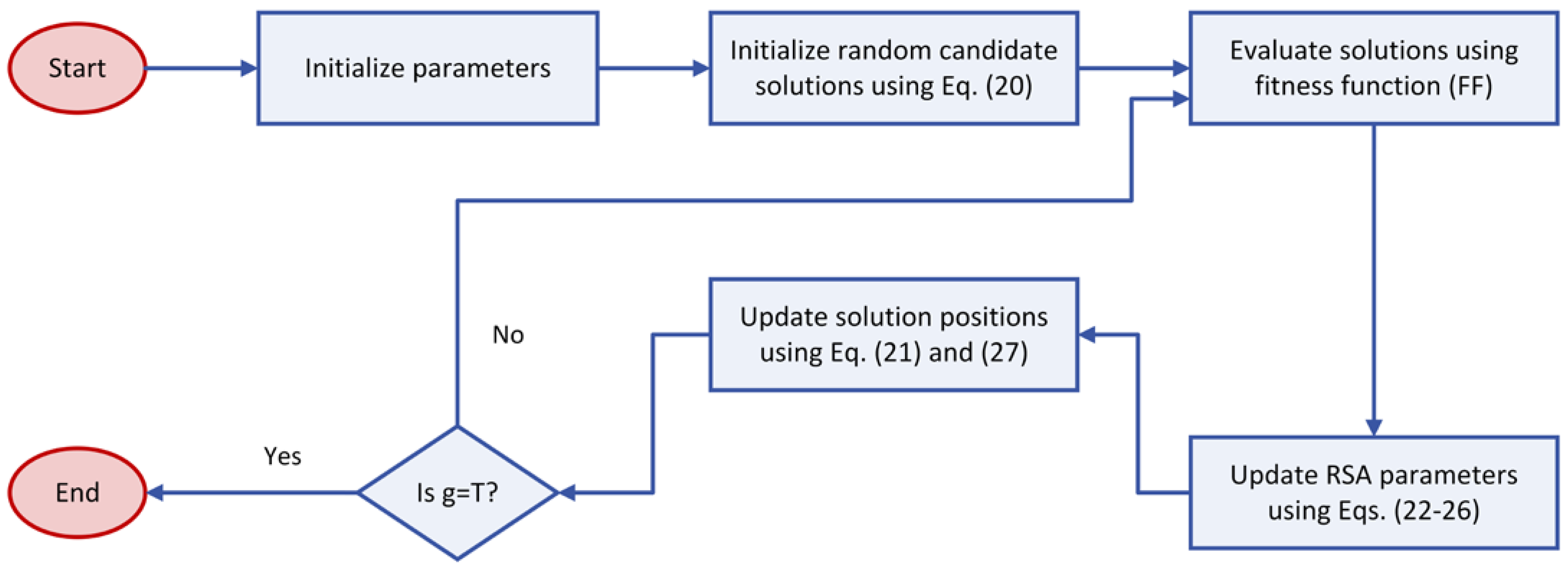
3.2.2. Reptile Search Algorithm (RSA)

RSA model is a popular modern nature-inspired model known as the reptile search algorithm (RSA); it is a metaheuristic algorithm inspired by the crocodiles’ encircling and hunting behavior. It was proposed in 2021 by [28] for the gradient-free algorithm with the generation of random solutions from the following equation [43,44].

$$x_{i,j}=ran{d}_{\in \left[0,1\right]}\times \left(U{B}_j-L{B}_j\right)+L{B}_j for i\in \left\{1,2,\dots ,N\right\} and j\in \left\{1,2,\dots ,M\right\}$$

(24)

Here, $x_{i,j}$ is the ith solution of the jth input for N solutions with M features, $ran{d}_{\in \left[0,1\right]}$ is a randomly produced number with uniform distribution ranging $\left[0,1\right]\left(0,1\right)$ and the jth property with $U{B}_j$, $L{B}_j$ taken as upper and lower boundaries.

As in all nature-inspired models, the RSA model also consists of exploration and exploitation principles. These two rules follow the crocodiles’ behavior for encircling the prey target for the RSA model. To adopt the crocodiles’ behavior, a four-iterations process has been considered. The first two stages of iterations are utilized on the basis of exploration for encompassing performance, including the high and the belly walking arrangements. The crocodiles start orbiting to hunt the area, enabling a further comprehensive hunt of the solution’s space. This encircling process can be modeled mathematically as:

$$\begin{array}{c}{x}_{i,j}\left(g+1\right)\hfill \\ =\{\begin{array}{c}\left[-{\eta }_{i,j}\left(g\right)\cdot \gamma \cdot Bes{t}_j\left(g\right)\right]-\left[{\mathit{rand}}_{\in \{1,N]}\cdot R_{i,j}\left(g\right)\right], \mathrm{for}g\le \frac{T}{4}\hfill \\ ES\left(g\right)\cdot Bes{t}_j\left(g\right)\cdot x_{\left(ran{d}_{\in \left[1, N\right],j}\right)}, \mathrm{for}g\le \frac{2T}{4} and g>\frac{T}{4}\hfill \end{array}\hfill \end{array}$$

(25)

Here, for the jth feature, $Bes{t}_j\left(g\right)$ is the finest result; with ith solution, $n_{i,j}$ is the hunting operator; to control the accuracy of exploration, $\gamma$ is used; $R_{i,j}\left(g\right)$ is used to compact and optimize search space; $ran{d}_{\in \left[1,N\right]}$ is used to randomize possible candidate solutions and $ES\left(g\right)$ used to reduce the probability ratio.

$$n_{i,j}=Bes{t}_j\left(g\right)\times P_{i,j}$$

(26)

$P_{i,j}$ is the fraction variance among the jth value of the finest result and the corresponding value in the current solution; it is evaluated below.

$$P_{i,j}=\theta +\frac{x_{i,j}-M\left(x_i\right)}{Bes{t}_j\left(g\right)\times \left(U{B}_j-L{B}_j\right)+\epsilon }$$

(37)

$\theta$ represents a sensitive factor to switches in the exploration performance; $M\left(x_i\right)$ denotes the mean solutions, and $\epsilon$ depicts small floor value, evaluated as below:

$$M\left(x_i\right)=\frac{1}{n}{\displaystyle \sum }_{j=1}^n{x}_{i,j}$$

(28)

$$R_{i,j}=\frac{Bes{t}_j\left(g\right)-x_{\left({\mathit{rand}}_{\epsilon \left[1,N\right]},j\right)}}{Bes{t}_j\left(g\right)+\epsilon }$$

(29)

$$ES\left(g\right)=2\times {\mathit{rand}}_{\in \left[-1,1\right]}\times \left(1-\frac{1}{T}\right)$$

(30)

Here, the multiple with 2 is used to deliver correlation values in [0, 2], and $ran{d}_{\in \left[-1,1\right]}$ is arbitrary in [–1, 1].

In last phase of iterations, the RSA model employs exploitation to search the solution’s space to find an optimal solution, which is directly dependent upon hunting coordination and cooperation. The below equations are used to update the optimal solution.

$$\begin{array}{c}{x}_{ij}\left(g+1\right)\hfill \\ =\{\begin{array}{c}\left[{\mathit{rand}}_{ϵ\{-1,1]}\cdot {\mathit{Best}}_j\left(g\right)\cdot P_{ij}\left(g\right)\right], \mathrm{for}g\le \frac{3T}{4} \mathrm{and} g>\frac{2T}{4}\hfill \\ \left[\epsilon \cdot {\mathit{Best}}_j\left(g\right)\cdot n_{ij}\left(g\right)\right]\left[\mathit{rand}{ϵ}_{\{-1,1]}\cdot R_{ij}\left(g\right)\right], \mathrm{for}g\le T \mathrm{and} g>\frac{3T}{4}\hfill \end{array}\hfill \end{array}$$

(31)

The performance of entrant solutions, obtained from every iteration, is obtained using pre-defined FF and the model stops the performance after the T iteration with the least fitness value (OFS). The path of the RSA model is described in Figure 4.

3.3. Improved Deep Learning Models

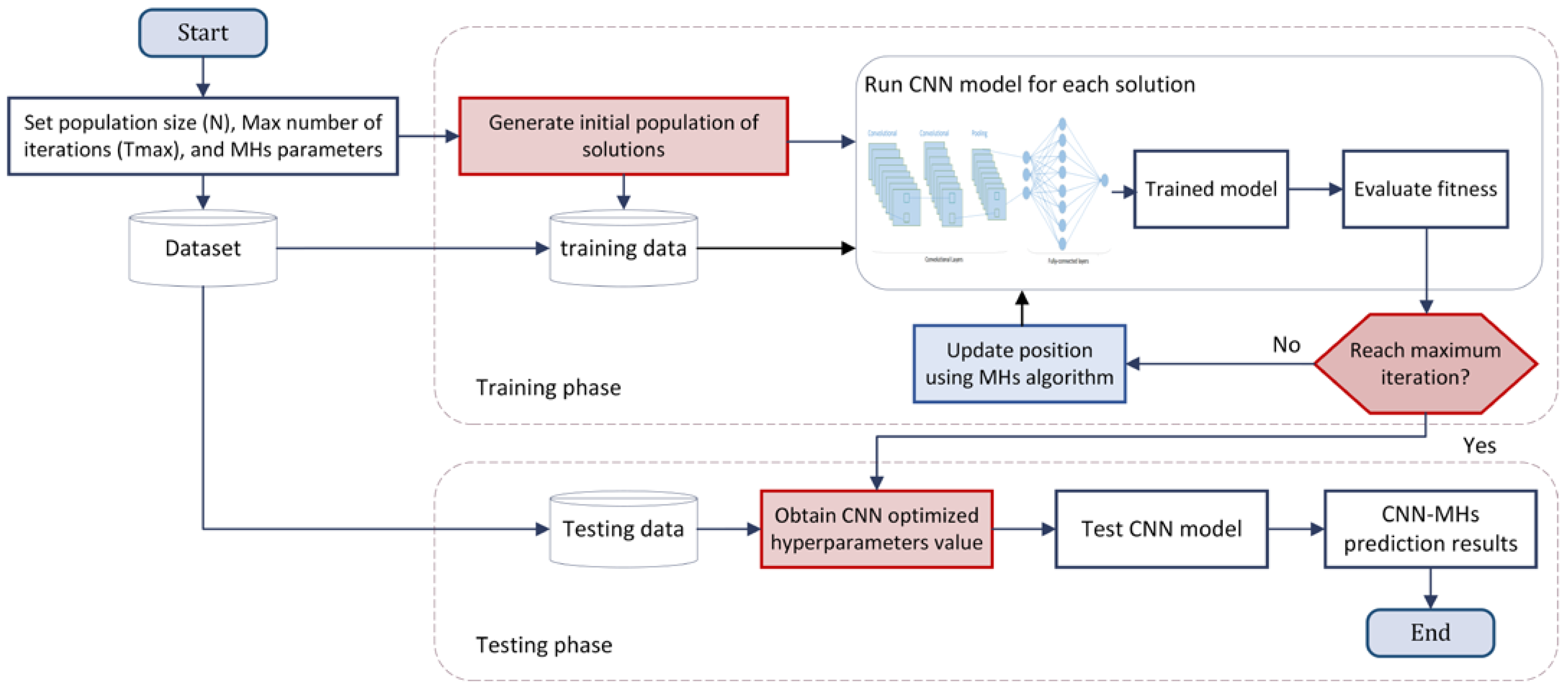
3.3.1. Improved CNN Model

To improve the performance of the CNN model, its hyperparameters were optimized using the MHs algorithm, namely RSA and INFO. To this end, first, the hyperparameters of 1D CNN were optimized using MHs based on training data. Then, the trained 1D CNN was used to predict unknown values in test data.

One-dimensional CNN has several hyperparameters, and its performance depends on their optimal values. The goal of using the MH algorithm in the proposed method is to find optimal deals for these hyperparameters, which leads to improved prediction accuracy. To this end, we consider five critical hyperparameters in the proposed method, including the number of filters, kernel size, number of epochs, batch size, and pooling size. These hyperparameters and their ranges are listed in

Table 2. List of hyperparameters and their values.

Number of filters	[1–300]
Kernel size	[1–20]
Number of epochs	[1–200]
Batch size	[10–100]
Pooling size	[1–15]

. Thus, each solution in the population space of this MHs algorithm contains five values corresponding to the considered parameters.

The optimization procedure has an initialization step in which several individuals are randomly produced as the positions. The number of places equals the number of CNN hyperparameters optimized using the MH algorithm. After this step (initialization), the searching process of the MH algorithm is repeated and the first populations (new generations) are computed to reach the best solution. This solution provides the optimal values of CNN hyperparameters. To assess the accuracy of each solution, the fitness function (FF) is applied. Here, the RMSE was employed as a FF.

After implementing the MH algorithm, the best solution (optimal CNN hyperparameters) is obtained. Then, the final optimized hyperparameter sets are passed to CNN to evaluate prediction ability. The general procedure of the CNN-MHs is provided in Figure 5.

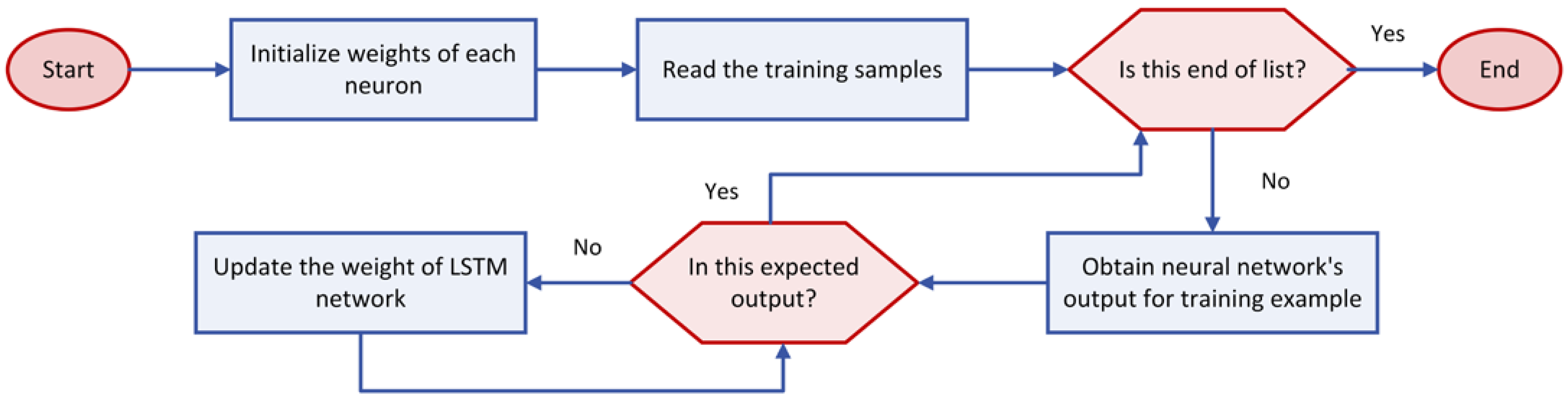
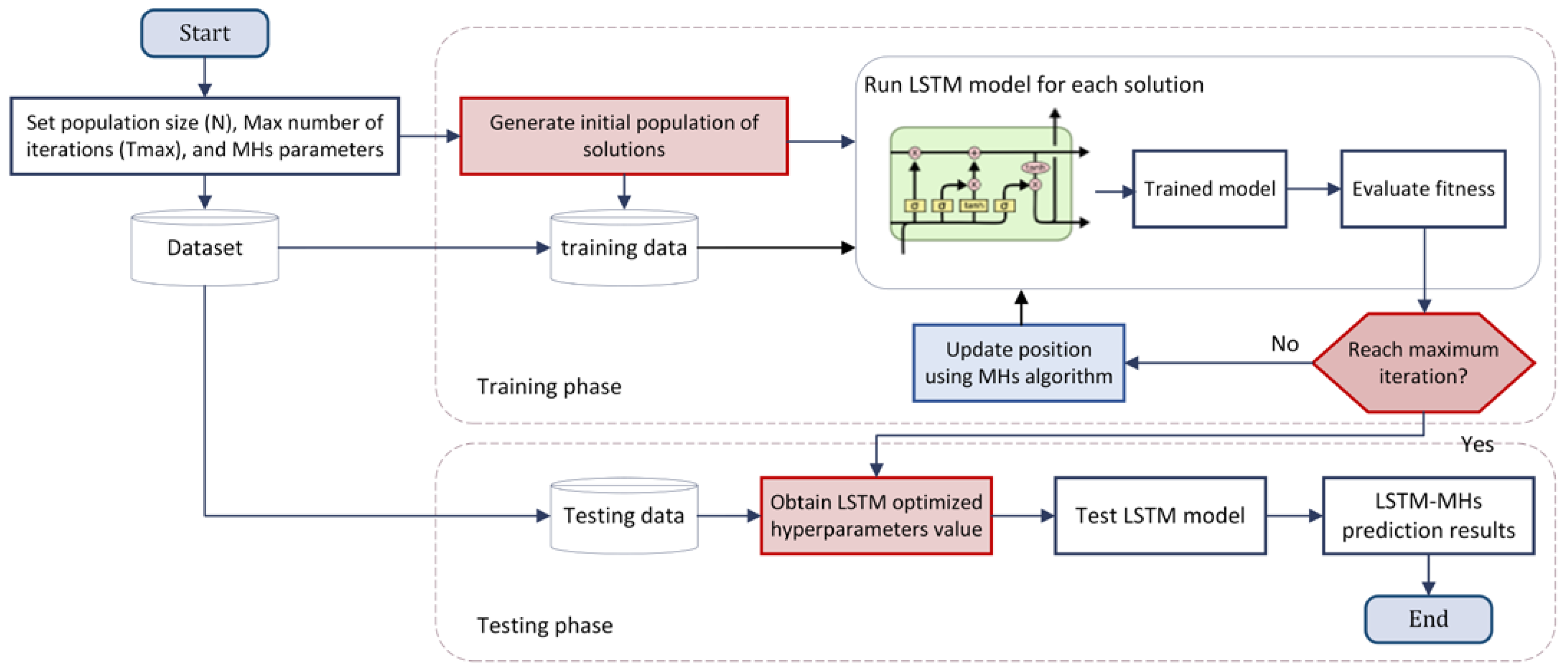
3.3.2. Improved LSTM Model

In this section, metaheuristic algorithms (MHs) are employed to develop a more accurate LSTM model (Figure 6). Two MHs, RSA and INFO, were used here to optimize the learning rate ( ) and hidden neurons ( ). This inclusion of RSA and INFO enhances the prediction accuracy more than the single LSTM model. Here, the dataset is divided into two groups: the training set (70%) and the testing set (30%). The proposed approach generates a solutions set involving the parameters of the LSTM. The fitness function RSME is then applied, which is formulated as below:

$$RMSE=\sqrt{\frac{1}{n}{\sum }_{i=1}^N{\left(a_i-p_i\right)}^2}$$

(32)

where a_i is the actual value, and p_i is the predicted value. After that, the solutions were updated according to the search mechanisms of the MHs, as described in the previous section. The best solution is the one that obtains the smallest RMSE value. The process of updating solutions is repeated until the terminal condition is met. In addition, the quality of the proposed LSTM-MHs is tested using 30% of the sample dataset (testing set) by employing the evaluation metrics to compute the prediction output.

The specific steps for using MHs to optimize LSTM parameters are as follows:

Step 1:

Split the input data into two groups to train and test the method.

Step 2:

Initialize the relevant parameters: population size (N), the maximum number of iterations (tmax), the upper and lower bounds of the search space ub and lb, respectively, and the range of LSTM parameters (h, α).

Step 3:

Generate the initial population of the solution.

Step 4:

Calculate the fitness value of each solution using LSTM training.

Step 5:

Use the MHs algorithm to optimize the hyperparameters of LSTM by exploring the search domain.

Step 6:

Use LSTM objective function to evaluate each candidate parameter.

Step 7:

The process is iterated until the maximum number of iterations is reached.

Step 8:

The final optimized set of hyperparameters is then passed to ELM to evaluate prediction ability.

4. Model Parameters and Accuracy Assessment

The following statistics were utilized for the assessment of the methods:

$$\mathrm{RMSE}:\mathrm{Root}\mathrm{Mean}\mathrm{Square}\mathrm{Error}=\sqrt{\frac{1}{\mathrm{N}}{\sum }_{\mathrm{i}=1}^{\mathrm{N}}{[{({\mathrm{Y}}_0)}_{\mathrm{i}}-{({\mathrm{Y}}_{\mathrm{C}})}_{\mathrm{i}}]}^2}$$

(33)

$$\mathrm{MAE}:\mathrm{Mean}\mathrm{Absolute}\mathrm{Error}=\frac{1}{\mathrm{N}}{\sum }_{\mathrm{i}=1}^{\mathrm{N}}|{({\mathrm{Y}}_0)}_{\mathrm{i}}-{({\mathrm{Y}}_{\mathrm{C}})}_{\mathrm{i}}|$$

(34)

$$\mathrm{NSE}:\mathrm{Nash}-\mathrm{Sutcliffe}\mathrm{Efficiency}=1-\frac{{\sum }_{\mathrm{i}=1}^{\mathrm{N}}{[{({\mathrm{Y}}_0)}_{\mathrm{i}}-{({\mathrm{Y}}_{\mathrm{c}})}_{\mathrm{i}}]}^2}{{\sum }_{\mathrm{i}=1}^{\mathrm{N}}{[{({\mathrm{Y}}_0)}_{\mathrm{i}}-{\overline{\mathrm{Y}}}_0]}^2},-\infty <\mathrm{NSE}\le 1$$

(35)

$${\mathrm{R}}^2:\mathrm{Determination}\mathrm{Coefficient}={\left[\frac{{\sum }_{\mathrm{t}=1}^{\mathrm{N}}\left({\mathrm{Y}}_{\mathrm{o}}-\overline{{\mathrm{Y}}_{\mathrm{o}}}\right)\left({\mathrm{Y}}_{\mathrm{c}}-\overline{{\mathrm{Y}}_{\mathrm{c}}}\right)}{\sqrt{{\sum }_{\mathrm{t}=1}^{\mathrm{N}}{({\mathrm{Y}}_{\mathrm{o}}-\overline{{\mathrm{Y}}_{\mathrm{o}}})}^2{({\mathrm{Y}}_{\mathrm{c}}-\overline{{\mathrm{Y}}_{\mathrm{c}}})}^2}}\right]}^2$$

(36)

where ${\mathrm{Y}}_{\mathrm{c}}, {\mathrm{Y}}_{\mathrm{o}}, {\overline{\mathrm{Y}}}_{\mathrm{o}}, \mathrm{N}$ are calculated, observed, mean water temperature and average of the observed streamflow and number of data, respectively. The parameters of both algorithms are listed in

Table 3. Parameter settings for all algorithms.

Algorithm	Parameter
RSA	$\alpha$	0.1
	$\beta$	0.1
INFO	$c$	2
	$d$	4
Common Settings	Population	30
	Number of iterations	100
	Number of runs for each algorithm	30

. For each algorithm, 30 populations and 100 iterations were used, and models were run 30 times to be able to obtain more robust outcomes. Data were split into three parts, M1, M2 and M3, and at each time, one part was used as testing and the other two used for training. Thus, the training and testing procedures scanned all the data.

5. Results and Discussion

This section provides the outcomes of the improved deep learning methods, convolutional neural networks (CNN) and long short-term memory (LSTM) network using the reptile search algorithm (RSA) and weighted mean of vectors optimizer (INFO) in predicting water temperature using different input combinations of air temperature, streamflow, precipitation, sediment flows and day of the year (DOY).

5.1. Results

Training and testing results of the single CNN models in water temperature prediction are summed up in

Table 4. Training and test statistics of the models for water temperature prediction—CNN.

Inputs Combinations	Training Period				Test Period
	RMSE	MAE	R2	NSE	RMSE	MAE	R2	NSE
M1
(i) Ta	1.554	1.211	0.914	0.914	1.652	1.289	0.918	0.894
(ii) Ta, P	1.453	1.120	0.925	0.924	1.689	1.302	0.917	0.889
(iii) Ta, Q	1.538	1.194	0.915	0.915	1.654	1.294	0.918	0.894
(iv) Ta, S	1.494	1.154	0.920	0.920	1.645	1.294	0.921	0.895
(v) Ta, P, Q	1.497	1.162	0.920	0.920	1.636	1.281	0.920	0.896
(vi) Ta, Q, S	1.477	1.140	0.922	0.922	1.675	1.310	0.917	0.891
(vii) Ta, P, Q, S	1.489	1.149	0.921	0.921	1.644	1.287	0.922	0.895
(viii) Ta, DOY	1.414	1.089	0.928	0.928	1.623	1.256	0.921	0.898
(ix) Ta, P, Q, S, DOY	1.376	1.067	0.934	0.934	1.567	1.223	0.928	0.905
Mean	1.475	1.141	0.922	0.922	1.643	1.282	0.920	0.895
M2
(i) Ta	1.434	1.119	0.924	0.924	1.559	1.248	0.927	0.926
(ii) Ta, P	1.384	1.075	0.929	0.929	1.512	1.191	0.937	0.936
(iii) Ta, Q	1.444	1.119	0.923	0.923	1.528	1.221	0.929	0.928
(iv) Ta, S	1.464	1.140	0.921	0.920	1.552	1.237	0.929	0.925
(v) Ta, P, Q	1.379	1.068	0.929	0.929	1.491	1.199	0.932	0.929
(vi) Ta, Q, S	1.434	1.112	0.924	0.924	1.585	1.240	0.931	0.928
(vii) Ta, P, Q, S	1.468	1.061	0.920	0.920	1.480	1.178	0.929	0.926
(viii) Ta, DOY	1.360	1.046	0.930	0.930	1.441	1.165	0.937	0.933
(ix) Ta, P, Q, S, DOY	1.417	1.100	0.926	0.925	1.514	1.179	0.925	0.924
Mean	1.422	1.096	0.925	0.925	1.527	1.204	0.931	0.928
M3
(i) Ta	1.433	1.113	0.930	0.929	1.446	1.136	0.933	0.929
(ii) Ta, P	1.479	1.138	0.925	0.925	1.345	1.067	0.939	0.937
(iii) Ta, Q	1.393	1.076	0.933	0.933	1.426	1.119	0.936	0.932
(iv) Ta, S	1.407	1.091	0.932	0.932	1.449	1.122	0.934	0.930
(v) Ta, P, Q	1.374	1.063	0.935	0.935	1.457	1.145	0.938	0.924
(vi) Ta, Q, S	1.403	1.083	0.932	0.932	1.423	1.109	0.931	0.916
(vii) Ta, P, Q, S	1.334	1.031	0.937	0.937	1.420	1.105	0.934	0.921
(viii) Ta, DOY	1.420	1.112	0.931	0.931	1.409	1.113	0.936	0.926
(ix) Ta, P, Q, S, DOY	1.331	1.020	0.939	0.939	1.395	1.096	0.942	0.935
Mean	1.397	1.081	0.933	0.933	1.418	1.112	0.936	0.934

for three different datasets and nine different input combinations. It is observed from the table that the CNN model offers the best accuracy for input combination ix involving all input parameters in M1 and M3 datasets, while input combination viii, with air temperature and day of the year, provided the lowest RMSE (1.441), MAE (1.165) and the highest R² (0.937), NSE (0.933) in predicting water temperature in the test period. Training statistics also keep the same trend. In all three subsets (M1, M2 and M3), adding DOY input considerably improved the model performance. For example, in the M2 set, adding DOY to the input combination vii improved the RMSE and MAE by 4.68% and 4.97%, and adding DOY to the input combination I in the M2 set improved the RMSE and MAE of the CNN model by 7.57% and 6.65% in the test period. As expected, the air temperature is the most effective factor influencing water temperature; therefore, it was kept in all input combinations.

Table 5. Training and test statistics of the models for water temperature prediction—CNN-RSA.

Inputs Combinations	Training Period				Test Period
	RMSE	MAE	R2	NSE	RMSE	MAE	R2	NSE
M1
(i) Ta	1.470	1.149	0.923	0.923	1.611	1.252	0.919	0.899
(ii) Ta, P	1.421	1.091	0.928	0.928	1.574	1.217	0.924	0.904
(iii) Ta, Q	1.451	1.112	0.925	0.925	1.594	1.229	0.920	0.902
(iv) Ta, S	1.477	1.143	0.922	0.922	1.620	1.260	0.919	0.898
(v) Ta, P, Q	1.399	1.077	0.930	0.930	1.600	1.258	0.925	0.901
(vi) Ta, Q, S	1.450	1.133	0.926	0.925	1.649	1.292	0.920	0.895
(vii) Ta, P, Q, S	1.401	1.080	0.930	0.930	1.584	1.254	0.929	0.903
(viii) Ta, DOY	1.388	1.080	0.933	0.931	1.557	1.212	0.928	0.906
(ix) Ta, P, Q, S, DOY	1.336	1.034	0.936	0.933	1.507	1.54	0.930	0.912
Mean	1.421	1.100	0.928	0.927	1.588	1.236	0.924	0.902
M2
(i) Ta	1.420	1.104	0.925	0.925	1.535	1.227	0.931	0.921
(ii) Ta, P	1.358	1.053	0.932	0.932	1.478	1.173	0.941	0.927
(iii) Ta, Q	1.419	1.098	0.925	0.925	1.526	1.216	0.931	0.922
(iv) Ta, S	1.436	1.114	0.924	0.923	1.548	1.232	0.934	0.920
(v) Ta, P, Q	1.376	1.053	0.930	0.930	1.471	1.163	0.938	0.928
(vi) Ta, Q, S	1.430	1.110	0.924	0.924	1.540	1.254	0.933	0.921
(vii) Ta, P, Q, S	1.413	1.096	0.926	0.926	1.474	1.146	0.937	0.928
(viii) Ta, DOY	1.352	1.047	0.932	0.932	1.452	1.173	0.937	0.930
(ix) Ta, P, Q, S, DOY	1.330	1.019	0.938	0.936	1.445	1.146	0.943	0.933
Mean	1.393	1.077	0.930	0.929	1.496	1.192	0.936	0.925
M3
(i) Ta	1.413	1.100	0.931	0.931	1.416	1.118	0.933	0.929
(ii) Ta, P	1.354	1.056	0.937	0.937	1.316	1.043	0.940	0.938
(iii) Ta, Q	1.370	1.064	0.936	0.935	1.419	1.116	0.934	0.928
(iv) Ta, S	1.389	1.077	0.934	0.934	1.399	1.093	0.933	0.930
(v) Ta, P, Q	1.317	1.009	0.941	0.940	1.330	1.032	0.941	0.937
(vi) Ta, Q, S	1.379	1.072	0.935	0.935	1.397	1.098	0.936	0.930
(vii) Ta, P, Q, S	1.324	1.020	0.940	0.940	1.365	1.069	0.940	0.934
(viii) Ta, DOY	1.279	1.002	0.945	0.944	1.266	0.978	0.947	0.943
(ix) Ta, P, Q, S, DOY	1.316	1.019	0.940	0.940	1.351	1.066	0.943	0.935
Mean	1.349	1.046	0.938	0.937	1.362	1.068	0.939	0.934

lists the training and testing statistics of the hybrid CNN-RSA models in predicting water temperature. In the M1 and M2 datasets, the input combination ix had the best accuracy, while the model produced the lowest RMSE (1.266), MAE (0.976) and the biggest R² (0.947), NSE (0.943) for the input combination viii in the test period. For this method (CNN-RSA), the DOY input also improves the prediction accuracy; improvement in RMSE is 4.86% from input combinations vii to ix in M1 set, while the corresponding percentage is 10.59% from input combinations i to viii in M3 set in the test period. The outcomes of the hybrid CNN-INFO models are summed up in

Table 6. Training and test statistics of the models for water temperature prediction—CNN-INFO.

Inputs Combinations	Training Period				Test Period
	RMSE	MAE	R2	NSE	RMSE	MAE	R2	NSE
M1
(i) Ta	1.450	1.131	0.925	0.925	1.606	1.243	0.922	0.900
(ii) Ta, P	1.413	1.089	0.929	0.929	1.573	1.218	0.925	0.904
(iii) Ta, Q	1.348	1.043	0.935	0.935	1.546	1.182	0.928	0.907
(iv) Ta, S	1.442	1.124	0.926	0.926	1.620	1.276	0.921	0.898
(v) Ta, P, Q	1.330	1.020	0.937	0.937	1.505	1.186	0.933	0.912
(vi) Ta, Q, S	1.358	1.054	0.935	0.934	1.561	1.222	0.927	0.905
(vii) Ta, P, Q, S	1.333	1.035	0.937	0.936	1.507	1.176	0.933	0.912
(viii) Ta, DOY	1.318	1.013	0.940	0.938	1.360	1.081	0.945	0.928
(ix) Ta, P, Q, S, DOY	1.369	1.051	0.933	0.933	1.538	1.188	0.928	0.908
Mean	1.373	1.062	0.933	0.932	1.535	1.197	0.929	0.908
M2
(i) Ta	1.425	1.108	0.925	0.925	1.515	1.225	0.931	0.923
(ii) Ta, P	1.334	1.030	0.934	0.934	1.451	1.148	0.942	0.930
(iii) Ta, Q	1.388	1.073	0.930	0.928	1.435	1.151	0.931	0.931
(iv) Ta, S	1.440	1.119	0.923	0.923	1.531	1.213	0.933	0.922
(v) Ta, P, Q	1.288	1.000	0.939	0.938	1.421	1.113	0.938	0.933
(vi) Ta, Q, S	1.326	1.044	0.936	0.935	1.525	1.214	0.934	0.922
(vii) Ta, P, Q, S	1.358	1.047	0.932	0.932	1.467	1.157	0.937	0.928
(viii) Ta, DOY	1.132	0.874	0.953	0.952	1.383	1.099	0.946	0.936
(ix) Ta, P, Q, S, DOY	1.303	1.016	0.937	0.937	1.403	1.109	0.938	0.934
Mean	1.333	1.034	0.934	0.934	1.459	1.159	0.937	0.929
M3
(i) Ta	1.404	1.090	0.932	0.932	1.414	1.112	0.936	0.929
(ii) Ta, P	1.337	1.036	0.939	0.939	1.275	0.993	0.943	0.942
(iii) Ta, Q	1.359	1.057	0.937	0.937	1.395	1.078	0.941	0.931
(iv) Ta, S	1.357	1.052	0.937	0.937	1.401	1.100	0.934	0.930
(v) Ta, P, Q	1.256	0.962	0.946	0.946	1.335	1.051	0.944	0.937
(vi) Ta, Q, S	1.378	1.066	0.935	0.935	1.382	1.086	0.935	0.932
(vii) Ta, P, Q, S	1.290	0.990	0.943	0.943	1.364	1.069	0.941	0.934
(viii) Ta, DOY	1.219	0.947	0.950	0.949	1.241	0.962	0.949	0.945
(ix) Ta, P, Q, S, DOY	1.276	0.996	0.944	0.944	1.351	1.067	0.944	0.935
Mean	1.320	1.022	0.940	0.940	1.351	1.058	0.941	0.935

in predicting water temperature. In all three subsets (M1, M2 and M3), the CNN-INFO model had the lowest RMSE and MAE and the highest R² and NSE for input combination viii involving air temperature and DOY parameters. Importing DOY into the model input improves the RMSE and MAE accuracies of the CNN-INFO (compare the input combinations i and viii) by 15.3% and 13% for M1, by 8.71% and 10.3% for M2, and by 12.2% and 13.5% for M3 in the test period.

Training and testing outcomes of the single and hybrid LSTM models in predicting water temperature are reported in

Table 7. Training and test statistics of the models for water temperature prediction—LSTM.

Inputs Combinations	Training Period				Test Period
	RMSE	MAE	R2	NSE	RMSE	MAE	R2	NSE
M1
(i) Ta	1.529	1.186	0.916	0.916	1.631	1.259	0.919	0.897
(ii) Ta, P	1.438	1.108	0.926	0.926	1.612	1.251	0.925	0.899
(iii) Ta, Q	1.438	1.118	0.926	0.926	1.580	1.233	0.926	0.903
(iv) Ta, S	1.500	1.160	0.919	0.919	1.639	1.281	0.919	0.896
(v) Ta, P, Q	1.400	1.079	0.930	0.930	1.592	1.243	0.925	0.902
(vi) Ta, Q, S	1.452	1.118	0.925	0.925	1.654	1.295	0.918	0.894
(vii) Ta, P, Q, S	1.414	1.089	0.928	0.928	1.595	1.251	0.925	0.901
(viii) Ta, DOY	1.499	1.162	0.920	0.920	1.614	1.261	0.934	0.899
(ix) Ta, P, Q, S, DOY	1.386	1.068	0.932	0.932	1.566	1.221	0.929	0.905
Mean	1.451	1.121	0.925	0.925	1.609	1.255	0.924	0.900
M2
(i) Ta	1.428	1.111	0.924	0.924	1.535	1.242	0.930	0.921
(ii) Ta, P	1.384	1.069	0.929	0.929	1.466	1.151	0.937	0.928
(iii) Ta, Q	1.444	1.119	0.923	0.923	1.525	1.216	0.932	0.922
(iv) Ta, S	1.429	1.115	0.924	0.924	1.587	1.272	0.933	0.916
(v) Ta, P, Q	1.383	1.071	0.929	0.929	1.537	1.218	0.935	0.921
(vi) Ta, Q, S	1.434	1.113	0.924	0.924	1.572	1.271	0.932	0.918
(vii) Ta, P, Q, S	1.379	1.070	0.929	0.929	1.523	1.202	0.936	0.923
(viii) Ta, DOY	1.440	1.118	0.923	0.923	1.558	1.258	0.932	0.919
(ix) Ta, P, Q, S, DOY	1.358	1.052	0.932	0.932	1.456	1.168	0.937	0.929
Mean	1.409	1.093	0.927	0.927	1.529	1.222	0.934	0.922
M3
(i) Ta	1.417	1.092	0.931	0.931	1.424	1.117	0.934	0.928
(ii) Ta, P	1.361	1.050	0.936	0.936	1.341	1.050	0.939	0.936
(iii) Ta, Q	1.380	1.067	0.935	0.935	1.422	1.107	0.935	0.928
(iv) Ta, S	1.402	1.088	0.932	0.932	1.428	1.110	0.928	0.927
(v) Ta, P, Q	1.328	1.056	0.936	0.935	1.363	1.088	0.934	0.934
(vi) Ta, Q, S	1.383	1.068	0.934	0.934	1.411	1.091	0.940	0.929
(vii) Ta, P, Q, S	1.328	1.024	0.939	0.939	1.365	1.068	0.935	0.934
(viii) Ta, DOY	1.393	1.081	0.933	0.933	1.405	1.110	0.931	0.930
(ix) Ta, P, Q, S, DOY	1.319	1.021	0.940	0.940	1.354	1.055	0.943	0.935
Mean	1.367	1.056	0.936	0.936	1.390	1.088	0.936	0.931

,

Table 8. Training and test statistics of the models for water temperature prediction—LSTM-RSA.

Inputs Combinations	Training Period				Test Period
	RMSE	MAE	R2	NSE	RMSE	MAE	R2	NSE
M1
(i) Ta	1.486	1.155	0.921	0.921	1.608	1.252	0.923	0.900
(ii) Ta, P	1.399	1.084	0.931	0.930	1.555	1.197	0.927	0.906
(iii) Ta, Q	1.400	1.089	0.930	0.930	1.549	1.165	0.921	0.907
(iv) Ta, S	1.368	1.078	0.933	0.933	1.623	1.286	0.925	0.898
(v) Ta, P, Q	1.332	1.035	0.940	0.936	1.556	1.220	0.930	0.906
(vi) Ta, Q, S	1.446	1.116	0.925	0.925	1.645	1.289	0.920	0.895
(vii) Ta, P, Q, S	1.400	1.082	0.930	0.930	1.586	1.242	0.925	0.902
(viii) Ta, DOY	1.180	0.914	0.950	0.950	1.520	1.175	0.939	0.910
(ix) Ta, P, Q, S, DOY	1.351	1.048	0.932	0.932	1.553	1.205	0.926	0.907
Mean	1.372	1.066	0.932	0.932	1.577	1.226	0.926	0.904
M2
(i) Ta	1.418	1.101	0.925	0.925	1.530	1.228	0.929	0.922
(ii) Ta, P	1.372	1.062	0.930	0.930	1.419	1.130	0.941	0.933
(iii) Ta, Q	1.314	1.015	0.936	0.936	1.437	1.147	0.933	0.931
(iv) Ta, S	1.384	1.077	0.929	0.929	1.501	1.214	0.936	0.925
(v) Ta, P, Q	1.327	1.028	0.935	0.935	1.426	1.122	0.939	0.932
(vi) Ta, Q, S	1.378	1.058	0.930	0.930	1.512	1.202	0.932	0.924
(vii) Ta, P, Q, S	1.378	1.073	0.930	0.930	1.463	1.152	0.940	0.929
(viii) Ta, DOY	1.027	0.799	0.961	0.961	1.176	0.921	0.945	0.939
(ix) Ta, P, Q, S, DOY	1.342	1.037	0.936	0.936	1.449	1.158	0.938	0.930
Mean	1.328	1.029	0.935	0.935	1.428	1.135	0.938	0.932
M3
(i) Ta	1.393	1.075	0.933	0.933	1.421	1.113	0.935	0.928
(ii) Ta, P	1.305	1.006	0.942	0.941	1.317	1.040	0.944	0.938
(iii) Ta, Q	1.354	1.056	0.937	0.937	1.392	1.082	0.942	0.931
(iv) Ta, S	1.394	1.089	0.934	0.933	1.375	1.064	0.942	0.933
(v) Ta, P, Q	1.314	1.013	0.941	0.941	1.328	1.015	0.944	0.937
(vi) Ta, Q, S	1.343	1.049	0.938	0.938	1.404	1.096	0.935	0.930
(vii) Ta, P, Q, S	1.325	1.021	0.940	0.940	1.314	1.031	0.941	0.939
(viii) Ta, DOY	1.138	0.861	0.956	0.955	1.112	0.866	0.949	0.942
(ix) Ta, P, Q, S, DOY	1.191	0.921	0.954	0.951	1.354	1.067	0.944	0.935
Mean	1.306	1.010	0.942	0.941	1.342	1.048	0.944	0.936

and

Table 9. Training and test statistics of the models for water temperature prediction—LSTM-INFO.

Model Inputs	Training Period				Test Period
	RMSE	MAE	R2	NSE	RMSE	MAE	R2	NSE
M1
(i) Ta	1.405	1.087	0.927	0.927	1.606	1.245	0.920	0.900
(ii) Ta, P	1.311	1.000	0.936	0.936	1.561	1.229	0.929	0.905
(iii) Ta, Q	1.270	0.963	0.940	0.940	1.445	1.105	0.931	0.919
(iv) Ta, S	1.371	1.076	0.930	0.930	1.574	1.246	0.927	0.904
(v) Ta, P, Q	1.248	0.967	0.942	0.942	1.457	1.142	0.936	0.918
(vi) Ta, Q, S	1.287	1.020	0.939	0.939	1.512	1.183	0.932	0.911
(vii) Ta, P, Q, S	1.338	1.059	0.934	0.934	1.476	1.145	0.936	0.916
(viii) Ta, DOY	1.161	0.889	0.950	0.950	1.256	1.010	0.955	0.939
(ix) Ta, P, Q, S, DOY	1.263	0.982	0.942	0.941	1.416	1.108	0.941	0.922
Mean	1.295	1.005	0.938	0.938	1.478	1.157	0.934	0.915
M2
(i) Ta	1.460	1.139	0.924	0.924	1.511	1.213	0.930	0.924
(ii) Ta, P	1.356	1.042	0.934	0.934	1.420	1.124	0.942	0.933
(iii) Ta, Q	1.285	0.976	0.941	0.941	1.484	1.208	0.931	0.927
(iv) Ta, S	1.453	1.137	0.925	0.924	1.487	1.198	0.935	0.926
(v) Ta, P, Q	1.261	0.971	0.943	0.943	1.402	1.116	0.940	0.935
(vi) Ta, Q, S	1.301	1.018	0.939	0.939	1.524	1.213	0.935	0.923
(vii) Ta, P, Q, S	1.256	0.982	0.944	0.944	1.459	1.149	0.938	0.929
(viii) Ta, DOY	1.076	0.798	0.959	0.959	1.290	1.008	0.960	0.945
(ix) Ta, P, Q, S, DOY	1.052	0.823	0.960	0.960	1.198	0.946	0.950	0.952
Mean	1.278	0.987	0.941	0.941	1.419	1.131	0.940	0.932
M3
(i) Ta	1.378	1.060	0.935	0.935	1.412	1.104	0.935	0.929
(ii) Ta, P	1.254	0.963	0.946	0.946	1.292	1.006	0.945	0.941
(iii) Ta, Q	1.279	0.978	0.944	0.944	1.394	1.087	0.942	0.931
(iv) Ta, S	1.330	1.034	0.939	0.939	1.390	1.078	0.942	0.931
(v) Ta, P, Q	1.245	0.964	0.947	0.947	1.326	1.046	0.949	0.937
(vi) Ta, Q, S	1.295	1.004	0.942	0.942	1.376	1.104	0.935	0.933
(vii) Ta, P, Q, S	1.258	0.971	0.946	0.946	1.339	1.058	0.942	0.936
(viii) Ta, DOY	0.957	0.721	0.968	0.968	1.079	0.839	0.956	0.959
(ix) Ta, P, Q, S, DOY	1.067	0.816	0.961	0.961	1.187	0.880	0.965	0.950
Mean	1.229	0.946	0.947	0.947	1.310	1.022	0.946	0.938

. It is visible from Table 7 that the single LSTM models with inputs of Ta, P, Q, S, DOY (input combination ix) offered the best accuracy in all subsets (M1 to M3). On the other hand, the hybrid LSTM-RSA models performed the best for the inputs of air temperature and DOY (input combination viii) in all testing subsets. For the LSTM-INFO, the model with Ta and DOY outperformed the other alternatives in M1 and M3, while in M2, the model acted as the best for the full inputs (input combination ix) in predicting water temperature. Similar to the CNN-based models, the accuracy of the LSTM model was also improved by adding DOY to the input combinations

Comparison of input combinations vii and ix reveals that adding DOY into the model inputs decreases the RMSE and MAE of LSTM by 1.82% and 2.4% in M1, by 4.4% and 2.83% in M2, and 0.81% and 1.22% in M3 in the test period. It is clear from Table 8 and Table 9 that the positive effect of DOY in the prediction performance of the hybrid LSTM models is higher. For example, the RMSE and MAE of LSTM-RSA decrease by 23.1% and 25% from input combination i to viii in the M2 testing dataset. The corresponding improvements in RMSE and MAE of LSTM-INFO are 21.8% and 18.9% for the M1 dataset (Table 3).

Table 10. Training and test statistics of the best input combinations of all applied models for water temperature prediction.

Model	Training Period				Test Period
	RMSE	MAE	R2	NSE	RMSE	MAE	R2	NSE
M1
CNN	1.376	1.067	0.934	0.934	1.567	1.223	0.928	0.905
CNN-RSA	1.336	1.034	0.936	0.933	1.507	1.54	0.930	0.912
CNN-INFO	1.318	1.013	0.940	0.938	1.360	1.081	0.945	0.928
Mean	1.343	1.038	0.937	0.935	1.478	1.281	0.934	0.915
LSTM	1.386	1.068	0.932	0.932	1.566	1.221	0.929	0.905
LSTM-RSA	1.180	0.914	0.950	0.950	1.520	1.175	0.939	0.910
LSTM-INFO	1.161	0.889	0.950	0.950	1.256	1.010	0.955	0.939
Mean	1.242	0.957	0.944	0.944	1.447	1.135	0.941	0.918
M2
CNN	1.360	1.046	0.930	0.930	1.441	1.165	0.937	0.933
CNN-RSA	1.330	1.019	0.938	0.936	1.445	1.146	0.943	0.930
CNN-INFO	1.132	0.874	0.953	0.952	1.383	1.099	0.946	0.936
Mean	1.274	0.980	0.940	0.939	1.423	1.137	0.942	0.933
LSTM	1.358	1.052	0.932	0.932	1.456	1.168	0.937	0.929
LSTM-RSA	1.027	0.799	0.961	0.961	1.116	0.866	0.955	0.959
LSTM-INFO	1.052	0.823	0.960	0.960	1.198	0.946	0.950	0.952
Mean	1.146	0.891	0.951	0.951	1.257	0.993	0.947	0.947
M3
CNN	1.331	1.020	0.939	0.939	1.395	1.096	0.942	0.935
CNN-RSA	1.279	1.002	0.945	0.944	1.266	0.978	0.947	0.943
CNN-INFO	1.219	0.947	0.950	0.949	1.241	0.962	0.949	0.945
Mean	1.276	0.990	0.945	0.944	1.301	1.012	0.946	0.941
LSTM	1.319	1.021	0.940	0.940	1.354	1.055	0.943	0.935
LSTM-RSA	1.138	0.861	0.956	0.955	1.112	0.866	0.949	0.942
LSTM-INFO	0.957	0.721	0.968	0.968	1.079	0.839	0.956	0.959
Mean	1.138	0.868	0.955	0.954	1.202	0.938	0.952	0.948

lists the training and testing accuracies of the single and hybrid CNN and LSTM models in predicting water temperature. The best models with the least RMSE, MAE and the biggest R2 and NSE were selected for comparison in this table. It is apparent from the mean statistics in Table 9 that the LSTM-based models outperform the CNN-based models in water temperature prediction in all three testing datasets. It is also clear that tuning parameters of deep leaning models, CNN and LSTM, with RSA and INFO considerably improves their accuracy. The INFO algorithm is generally superior to the RSA in improving deep leaning models in water temperature prediction.

Figure 7 illustrates the scatterplots of the observed and predicted water temperatures using different CNN- and LSTM-based models in the test period. It is visible from the graphs that the hybrid CNN and LSTM models have less scattered predictions and higher R² compared to single models, and that the LSTM-INFO has the best predictions. It is clear from the Taylor diagram provided in Figure 8 and Figure 9 that the hybrid INFO algorithm-based LSTM and CNN model has the lowest RMSE and highest correlation, and its standard deviation is closer to the observed one compared to other alternative models. Single models are weaker than the hybrid deep learning models. It is visible from the violin charts given in Figure 10 and Figure 11 that the LSTM-INFO and CNN-INFO has closer distribution to that of the observed water temperature, indicating the capability of this method among the implemented methods.

5.2. Discussion

It was observed from the outcomes of the overall results that both the RSA and INFO algorithms considerably improved the deep learning methods in the prediction of water temperature; improvements in RMSE of the best CNN model for M3 dataset are 9.25% and 11.04% by applying RSA and INFO in the test period, and the corresponding percentages were 17.9% and 20.3% for the LSTM model in the same dataset. The LSTM-based models provided better efficiency than the CNN-based models, and the LSTM-INFO generally acted as the best model in the prediction of water temperature, improving the prediction accuracy of CNN, CNN-RSA, CNN-INFO, LSTM and LSTM-RSA models by 9.9%, 16.7%, 7.65%, 19.8% and 17.4% in the test period, respectively. The outcomes reveal the need for new metaheuristic algorithms in tuning hyperparameters of deep leaning methods (e.g., CNN and LSTM) for accurately predicting water temperature.

This was observed from the models’ results for various input combinations, considering DOY is very effective parameter and the prediction accuracy is considerably improved by involving this in the inputs. However, adding some input parameters deteriorates the prediction accuracy of the deep leaning models in all three testing datasets. For example, the RMSE and MAE of the CNN model increase from 1.652 and 1.289 to 1.689 and 1.302 by adding the precipitation parameter into the air temperature input (see input combinations i and ii in Table 4).

According to the previous studies [45,46], better prediction accuracy is not guaranteed by increasing the input number and, in some cases, this process may negatively affects the variance and may lead to more complicated models that provide a lower prediction accuracy. Another important piece of information that can be drawn from the outcomes of the presented study is the use of three different testing datasets. It was observed that the accuracies of the implemented models are highly variable with respect to three testing datasets. For example, the mean RMSE of CNN model varies from 1.643 to 1.418 between the M1 and M3 datasets, and this range is 1.609–1.390 for the LSTM model. A similar variation is also observed for the hybrid deep learning methods. All these suggest the use of different datasets in assessing machine learning methods and that the use of only one training–testing datasets, as is generally applied in the literature, can mislead the modeler.

Similar to the previous works [47,48], the outcomes of the present study revealed that the air temperature is the most important parameter in predicting water temperature. Our study also has direct agreement with those of Webb et al. [47] and Sohrabi et al. [49], as regards the discharge being the second most important parameter. The main drawback of the proposed methods is their data-driven nature. They cannot consider the impacts of possible changes in vegetation or other variables on stream water temperature, and if the testing data are far from the calibration period, the proposed methods may not work well. In such cases, the methods should be re-calibrated by taking into account the new variables which involve the quantitative information of the possible changes.

Zhu et al. (2018) [19] compared the accuracy of ANN and ANFIS in predicting river water temperature of three stations using air temperature, river flow discharge and the components of the Gregorian calendar as inputs. They obtained R² of 0.954 from the best model (ANN) as 0.954, 0.943 and 0.976 for three stations. Grbic et al. (2013) [11] investigated the prediction of water temperature of the Drava river in Croatia. They used inputs of air temperature, river flow discharge and the best model produced the NSE of 0.984. The hybrid models investigated in the presented study also provided high R² and NSE values (higher than 0.900). The lower accuracy of the improved CNN and LSTM models might be due to the fact that the previous studies did not consider cross-validation as we de did in our study, which causes a decrease in accuracy but provides more robust analysis.

6. Conclusions

Water temperature plays a key role in the precise management of river ecology and in keeping the balance between the ecosystems of aquatic life. In this study, two deep learning methods, namely convolutional neural networks (CNN) and long short-term memory (LSTM) network models, were evaluated to predict the daily water temperatures data of the Bailong River in China. To improve the prediction accuracy of both deep learning models, two recently developed optimization algorithms, i.e., the reptile search algorithm (RSA) and weighted mean of vectors optimizer (INFO), were utilized. Different input combinations of air temperature, streamflow, precipitation, sediment flows and day of the year (DOY) were analyzed on the basis of cross-validation to model water temperature data and the accuracy of modeling was accessed based on the root mean square errors (RMSE), mean absolute errors, determination coefficient and Nash–Sutcliffe efficiency statistics. It was found that a DOY input combination and INFO-based CNN provided more accurate results in comparison with other CNN based models. The RMSE and MAE accuracies of the other CNN-based models improved by 15.3–8.71% and 13.5–10.3% for all datasets through the use of DOY input combination in the CNN-INFO model. For the LSTM-based models, it was also found that INFO-based LSTM model outperformed the other competing LSTM-based model; however, inputs of air temperature and DOY yield more precise results in comparison with other inputs combinations. The LSTM-INFO model using Ta and DOY inputs reduced the RMSE and MAE errors of the other LSTM-based models by 25.1–21.8% and 23.4–18.9% for all datasets. It was also found that overall LSTM-INFO produced more precise results in comparison with CNN-INFO models. Proposed methods can be utilized to model other hydrological variables. They can also be used with decomposition techniques to capture noise in data in order to improve further prediction accuracy of the models.

References

- Caissie, D. The thermal regime of rivers: A review. Freshw. Biol. 2006, 51, 1389–1406. [Google Scholar] [CrossRef]
- Sahoo, G.; Schladow, S.; Reuter, J. Forecasting stream water temperature using regression analysis, artificial neural network, and chaotic non-linear dynamic models. J. Hydrol. 2009, 378, 325–342. [Google Scholar] [CrossRef]
- Bernhardt, E.S.; Heffernan, J.B.; Grimm, N.B.; Stanley, E.H.; Harvey, J.W.; Arroita, M.; Appling, A.; Cohen, M.J.; McDowell, W.H.; Hall, R.O.; et al. The metabolic regimes of flowing waters. Limnol. Oceanogr. 2017, 63, S99–S118. [Google Scholar] [CrossRef] [Green Version]
- Wanders, N.; Wada, Y. Human and climate impacts on the 21st century hydrological drought. J. Hydrol. 2015, 526, 208–220. [Google Scholar] [CrossRef]
- Wanders, N.; Van Vliet, M.T.H.; Wada, Y.; Bierkens, M.F.P.; Van Beek, L.P.H. High-Resolution Global Water Temperature Modeling. Water Resour. Res. 2019, 55, 2760–2778. [Google Scholar] [CrossRef]
- Liu, S.; Xu, L.; Li, D. Multi-scale prediction of water temperature using empirical mode decomposition with back-propagation neural networks. Comput. Electr. Eng. 2016, 49, 1–8. [Google Scholar] [CrossRef]
- Cai, H.; Piccolroaz, S.; Huang, J.; Liu, Z.; Liu, F.; Toffolon, M. Quantifying the impact of the Three Gorges Dam on the thermal dynamics of the Yangtze River. Environ. Res. Lett. 2018, 13, 054016. [Google Scholar] [CrossRef]
- Du, X.; Shrestha, N.K.; Wang, J. Assessing climate change impacts on stream temperature in the Athabasca River Basin using SWAT equilibrium temperature model and its potential impacts on stream ecosystem. Sci. Total. Environ. 2019, 650, 1872–1881. [Google Scholar] [CrossRef]
- Sartori, E. A Mathematical Model for Predicting Heat and Mass Transfer from a Free Water Surface. In Advances in Solar Energy Technology; Pergamon: Oxford, UK, 1988; pp. 3160–3164. [Google Scholar] [CrossRef]
- Caissie, D.; El-Jabi, N.; St-Hilaire, A. Stochastic modelling of water temperatures in a small stream using air to water relations. Can. J. Civ. Eng. 1998, 25, 250–260. [Google Scholar] [CrossRef]
- Grbić, R.; Kurtagić, D.; Slišković, D. Stream water temperature prediction based on Gaussian process re-gression. Expert Syst. Appl. 2013, 40, 7407–7414. [Google Scholar] [CrossRef]
- Parmar, K.S.; Bhardwaj, R. Water quality management using statistical analysis and time-series predic-tion model. Appl. Water Sci. 2014, 4, 425–434. [Google Scholar] [CrossRef] [Green Version]
- Tiyasha, T.; Tung, T.M.; Bhagat, S.K.; Tan, M.L.; Jawad, A.H.; Mohtar WH, M.W.; Yaseen, Z.M. Func-tionalization of remote sensing and on-site data for simulating surface water dissolved oxygen: Development of hy-brid tree-based artificial intelligence models. Mar. Pollut. Bull. 2021, 170, 112639. [Google Scholar] [CrossRef] [PubMed]
- Quan, Q.; Hao, Z.; Xifeng, H.; Jingchun, L. Research on water temperature prediction based on improved sup-port vector regression. Neural Comput. Appl. 2022, 34, 8501–8510. [Google Scholar] [CrossRef]
- Alizamir, M.; Kisi, O.; Adnan, R.M.; Kuriqi, A. Modelling reference evapotranspiration by combining neuro-fuzzy and evolutionary strategies. Acta Geophys. 2020, 68, 1113–1126. [Google Scholar] [CrossRef]
- Yuan, X.; Chen, C.; Lei, X.; Yuan, Y.; Muhammad Adnan, R. Monthly runoff forecasting based on LSTM–ALO model. Stoch. Environ. Res. Risk Assess. 2018, 32, 2199–2212. [Google Scholar] [CrossRef]
- Ikram, R.M.A.; Dai, H.-L.; Ewees, A.A.; Shiri, J.; Kisi, O.; Zounemat-Kermani, M. Application of improved version of multi verse optimizer algorithm for modeling solar radiation. Energy Rep. 2022, 8, 12063–12080. [Google Scholar] [CrossRef]
- Adnan, R.M.; Kisi, O.; Mostafa, R.R.; Ahmed, A.N.; El-Shafie, A. The potential of a novel support vector machine trained with modified mayfly optimization algorithm for streamflow prediction. Hydrol. Sci. J. 2022, 67, 161–174. [Google Scholar] [CrossRef]
- Zhu, S.; Nyarko, E.K.; Hadzima-Nyarko, M. Modelling daily water temperature from air temperature for the Missouri River. Peerj 2018, 6, e4894. [Google Scholar] [CrossRef] [Green Version]
- Zhu, S.; Nyarko, E.K.; Hadzima-Nyarko, M.; Heddam, S.; Wu, S. Assessing the performance of a suite of machine learning models for daily river water temperature prediction. Peerj 2019, 7, e7065. [Google Scholar] [CrossRef]
- Zhu, S.; Heddam, S.; Nyarko, E.K.; Hadzima-Nyarko, M.; Piccolroaz, S.; Wu, S. Modeling daily water temperature for rivers: Comparison between adaptive neuro-fuzzy inference systems and artificial neural networks models. Environ. Sci. Pollut. Res. 2018, 26, 402–420. [Google Scholar] [CrossRef]
- Han, M.; Feng, Y.; Zhao, X.; Sun, C.; Hong, F.; Liu, C. A Convolutional Neural Network Using Surface Data to Predict Subsurface Temperatures in the Pacific Ocean. IEEE Access 2019, 7, 172816–172829. [Google Scholar] [CrossRef]
- Ikram, R.M.A.; Mostafa, R.R.; Chen, Z.; Islam, A.R.M.T.; Kisi, O.; Kuriqi, A.; Zounemat-Kermani, M. Advanced Hybrid Metaheuristic Machine Learning Models Application for Reference Crop Evapotranspiration Prediction. Agronomy 2023, 13, 98. [Google Scholar] [CrossRef]
- Zounemat-Kermani, M.; Keshtegar, B.; Kisi, O.; Scholz, M. Towards a comprehensive assessment of statis-tical versus soft computing models in hydrology: Application to monthly pan evaporation prediction. Water 2021, 13, 2451. [Google Scholar] [CrossRef]
- Mahdavi-Meymand, A.; Sulisz, W.; Zounemat-Kermani, M. A comprehensive study on the application of firefly algorithm in prediction of energy dissipation on block ramps. Eksploat. I Niezawodn. 2022, 24, 200–210. [Google Scholar] [CrossRef]
- Qiu, R.; Wang, Y.; Wang, D.; Qiu, W.; Wu, J.; Tao, Y. Water temperature forecasting based on modified artificial neural network methods: Two cases of the Yangtze River. Sci. Total. Environ. 2020, 737, 139729. [Google Scholar] [CrossRef]
- Stajkowski, S.; Kumar, D.; Samui, P.; Bonakdari, H.; Gharabaghi, B. Genetic-Algorithm-Optimized Sequential Model for Water Temperature Prediction. Sustainability 2020, 12, 5374. [Google Scholar] [CrossRef]
- Abualigah, L.; Abd Elaziz, M.; Sumari, P.; Geem, Z.W.; Gandomi, A.H. Reptile Search Algorithm (RSA): A nature-inspired meta-heuristic optimizer. Expert Syst. Appl. 2022, 191, 116158. [Google Scholar] [CrossRef]
- Almotairi, K.H.; Abualigah, L. Improved reptile search algorithm with novel mean transition mechanism for constrained industrial engineering problems. Neural Comput. Appl. 2022, 34, 17257–17277. [Google Scholar] [CrossRef]
- Al-Shourbaji, I.; Helian, N.; Sun, Y.; Alshathri, S.; Abd Elaziz, M. Boosting Ant Colony Optimization with Rep-tile Search Algorithm for Churn Prediction. Mathematics 2022, 10, 1031. [Google Scholar] [CrossRef]
- Khan, R.A.; Sabir, B.; Sarwar, A.; Liu, H.D.; Lin, C.H. Reptile Search Algorithm (RSA)-Based Selective Har-monic Elimination Technique in Packed E-Cell (PEC-9) Inverter. Processes 2022, 10, 1615. [Google Scholar] [CrossRef]
- Ahmadianfar, I.; Heidari, A.A.; Noshadian, S.; Chen, H.; Gandomi, A.H. INFO: An efficient optimization al-gorithm based on weighted mean of vectors. Expert Syst. Appl. 2022, 195, 116516. [Google Scholar] [CrossRef]
- Hassan, A.Y.; Ismaeel, A.A.K.; Said, M.; Ghoniem, R.M.; Deb, S.; Elsayed, A.G. Evaluation of Weighted Mean of Vectors Algorithm for Identification of Solar Cell Parameters. Processes 2022, 10, 1072. [Google Scholar] [CrossRef]
- Hubel, D.H.; Wiesel, T.N. Receptive fields of single neurons in cat’s striate cortex. J. Physiol. 1959, 148, 1959. [Google Scholar] [CrossRef] [PubMed]
- Hubel, D.H.; Wiesel, T.N. Receptive fields and functional architecture of monkey striate cortex. J. Physiol. 1968, 195, 215–243. [Google Scholar] [CrossRef]
- Fukushima, K. Neocognitron: A self-organizing neural network model for a mechanism of pattern recognition unaffected by shift in position. Biol. Cybern. 1980, 36, 193–202. [Google Scholar] [CrossRef]
- Nair, V.; Hinton, G.E. Rectified linear units improve restricted boltzmann machines. In Proceedings of the 27th International Conference on International Conference on Machine Learning (ICML’10), Haifa, Israel, 21–24 June 2010; Omnipress: Haifa, Israel, 2010; pp. 807–814. [Google Scholar]
- Graves, A.; Schmidhuber, J. Framewise phoneme classification with bidirectional LSTM and other neural network architectures. Neural Netw. 2005, 18, 602–610. [Google Scholar] [CrossRef]
- Sundermeyer, M.; Schlüter, R.; Ney, H. From feedforward to recurrent. LSTM neural networks for language modeling. IEEE/ACM Trans. Audio Speech Lang. Process. 2015, 23, 517–529. [Google Scholar] [CrossRef]
- Gensler, A.; Henze, J.; Sick, B.; Raabe, N. Deep Learning for solar power forecasting—An approach using AutoEncoder and LSTM Neural Networks. In Proceedings of the 2016 IEEE International Conference, Systems, Man, and Cybernetics (SMC), Budapest, Hungary, 9 October 2016. [Google Scholar] [CrossRef]
- Nelson, D.M.Q.; Pereira, A.C.M.; de Oliveira, R.A. Stock market’s price movement prediction with LSTM neural networks. In Proceedings of the 2017 International Joint Conference on Neural Networks (IJCNN), Anchorage, AK, USA, 14–19 June 2017; pp. 1419–1426. [Google Scholar] [CrossRef]
- Adnan, R.M.; Liang, Z.; Heddam, S.; Zounemat-Kermani, M.; Kisi, O.; Li, B. Least square support vector machine and multivariate adaptive regression splines for streamflow prediction in mountainous basin using hydro-meteorological data as inputs. J. Hydrol. 2020, 586, 124371. [Google Scholar] [CrossRef]
- Elgamal, Z.; Sabri, A.Q.M.; Tubishat, M.; Tbaishat, D.; Makhadmeh, S.N.; Alomari, O.A. Improved Reptile Search Optimization Algorithm Using Chaotic Map and Simulated Annealing for Feature Selection in Medical Field. IEEE Access 2022, 10, 51428–51446. [Google Scholar] [CrossRef]
- Al-Shourbaji, I.; Kachare, P.H.; Alshathri, S.; Duraibi, S.; Elnaim, B.; Elaziz, M.A. An Efficient Parallel Reptile Search Algorithm and Snake Optimizer Approach for Feature Selection. Mathematics 2022, 10, 2351. [Google Scholar] [CrossRef]
- Shi, J.; Guo, J.; Zheng, S. Evaluation of hybrid forecasting approaches for wind speed and power generation time series. Renew. Sustain. Energy Rev. 2012, 16, 3471–3480. [Google Scholar] [CrossRef]
- Zhang, D.; Peng, X.; Pan, K.; Liu, Y. A novel wind speed forecasting based on hybrid decomposition and online sequential outlier robust extreme learning machine. Energy Convers. Manag. 2018, 180, 338–357. [Google Scholar] [CrossRef]
- Webb, B.W.; Clack, P.D.; Walling, D.E. Water-air temperature relationships in a Devon river system and the role of flow. Hydrol. Process. 2003, 17, 3069–3084. [Google Scholar] [CrossRef]
- Ahmadi-Nedushan, B.; St-Hilaire, A.; Ouarda, T.B.M.J.; Bilodeau, L.; Robichaud, E.; Thiemonge, N.; Bobee, B. Predicting river water temperatures using stochastic models: Case study of the Moisie River (Qu’ebec, Cana-da). Hydrol. Process. 2007, 21, 21–34. [Google Scholar] [CrossRef]
- Sohrabi, M.M.; Benjankar, R.; Tonina, D.; Wenger, S.J.; Isaak, D.J. Estimation of daily stream water temperatures with a Bayesian regression approach. Hydrol. Process. 2017, 31, 1719–1733. [Google Scholar] [CrossRef]