Article

A New Boundary Condition Framework for Particle Method by Using Local Regular-Distributed Background Particles—The Special Case for Poisson Equation

1
School of Naval Architecture and Ocean Engineering, Dalian University of Technology, Dalian 116024, China
2
Dalian Shipbuilding Industry Co., Ltd., Dalian 116021, China
3
State Key Laboratory of Structural Analysis for Industrial Equipment, Dalian 116024, China
4
Collaborative Innovation Center for Advanced Ship and Deep-Sea Exploration, Shanghai 200240, China
5
Faculty of Engineering and Physical Sciences, University of Southampton, Southampton SO16 7QF, UK
*
Authors to whom correspondence should be addressed.
J. Mar. Sci. Eng. 2023, 11(11), 2183; https://doi.org/10.3390/jmse11112183
Submission received: 14 October 2023 / Revised: 9 November 2023 / Accepted: 14 November 2023 / Published: 16 November 2023

Abstract

:
To improve the accuracy of solving the Poisson equation and the efficiency of handling complex boundary shapes in the particle method, this paper proposes a Local Regular-distributed Background Particles (LRBP) as an alternative to traditional boundary handling methods. This method avoids the trouble of arranging virtual particles by introducing background particles, making it suitable for problems with complex boundary shapes. In addition, based on the framework of the weak form Poisson equation, the boundary conditions are easily applied, and the calculations are more accurate. Furthermore, this method allows for different interpolation methods inside and outside the boundary, providing flexibility and versatility. These characteristics are well demonstrated in the validation examples, which indicate its potential to solve complex flow problems.

1. Introduction

In the field of ship and ocean engineering, there are numerous free-surface flow problems. However, traditional grid-based methods face challenges in terms of time-consuming grid generation and grid distortion when dealing with such problems. In these cases, various particle (meshless) methods have been proposed. Particle methods discretize the computational domain using arbitrarily distributed particles, and information such as mass, momentum, and pressure in fluid dynamics is carried by the moving particles. These particles evolve in time steps in a Lagrangian manner to track fluid motion and simulate fluid dynamics by considering interactions among particles. This makes particle methods uniquely advantageous in dealing with complex flow problems involving intricate moving boundaries and significant free-surface deformations, and they have been successfully applied to simulations involving sloshing in a liquid tank [1,2,3], water impact [4,5,6], and fluid–structure interaction problems [7,8,9], etc.
However, the particle method itself also has some limitations. In the mainstream particle methods, such as the ISPH (Incompressible Smoothed Particle Hydrodynamics) [10] and MPS (Moving particle Semi-implicit) [11] methods, the pressure field is obtained by solving the Poisson equation, and the accuracy of the pressure calculation depends on the solution of the Poisson equation [12,13,14]. Neumann boundary conditions or Dirichlet boundary conditions [15,16,17,18] are often required for the solution of the Poisson equation. Hence, accurately applying boundary conditions is a crucial challenge.
The virtual particle method (abbreviated as VPM), proposed by Koshizuka and Oka [11], is the most widely used wall boundary condition, which adds several layers of virtual particles around solid boundaries to supplement the density of fluid particles. The innermost boundary particles participate in solving the Poisson equation and achieve the no-slip condition by setting their velocities to zero. The outermost particles do not contribute to the solution of the Poisson equation, but their pressure values are set as equal to those of the nearest fluid particles. This approach effectively avoids particle penetration but increases the computational costs and is difficult to apply to complex-shaped boundaries.
The mirror particle method is another commonly used solid boundary treatment method that can be traced back to the work of Xie et al. [16]. When internal fluid particles approach the boundary, mirror particles with the same density and pressure but opposite velocities are generated outside the solid boundary. These mirror particles are then applied as Neumann boundary conditions on the solid boundary. Unlike the virtual particle method, the mirror particle method does not require additional virtual particles but incurs additional computational costs to calculate the positions of mirror particles.
From the above, it can be observed that there are still some issues with the current approaches for handling boundary conditions, such as insufficient support domain particles and difficulties representing complex boundary shapes. To address these problems, this paper proposes a new boundary treatment method that avoids the placement of virtual particles and is applicable to representing complex boundary shapes. Specifically, the method involves placing background particles at the boundary and applying boundary conditions based on these background particles, as well as the realization of information transfer between fluid particles and boundary particles.
The remaining sections of this article are arranged as follows: Section 2 mainly introduces the core of this article, which is the application boundary condition algorithm based on the local regular-distribution background particles, and provides detailed explanations of its implementation details. In Section 3, the convergence accuracy, different internal particle distributions, and irregular boundary shapes of the method are verified through the Taylor–Green vortex problem, demonstrating the feasibility and accuracy of the background particle method.

2. Methodology

2.1. Governing Equations

In the incompressible type meshless methods, such as ISPH and MPS, the pressure field is usually calculated by the pressure Poisson equation, as follows:
2 p = b ,
in which 2 is the Laplacian operator, p is the pressure field, and b is the known source term.
Normally, this Poisson equation is subject to the following Neumann or Dirichlet boundary conditions:
p n = p n = q on   Γ N e u m a n n p = p ¯ on   Γ D i r i c h l e t .
This paper aims to find an effective way to accurately impose these boundary conditions while preserving the Lagrangian and meshless properties in the particle methods as much as possible.

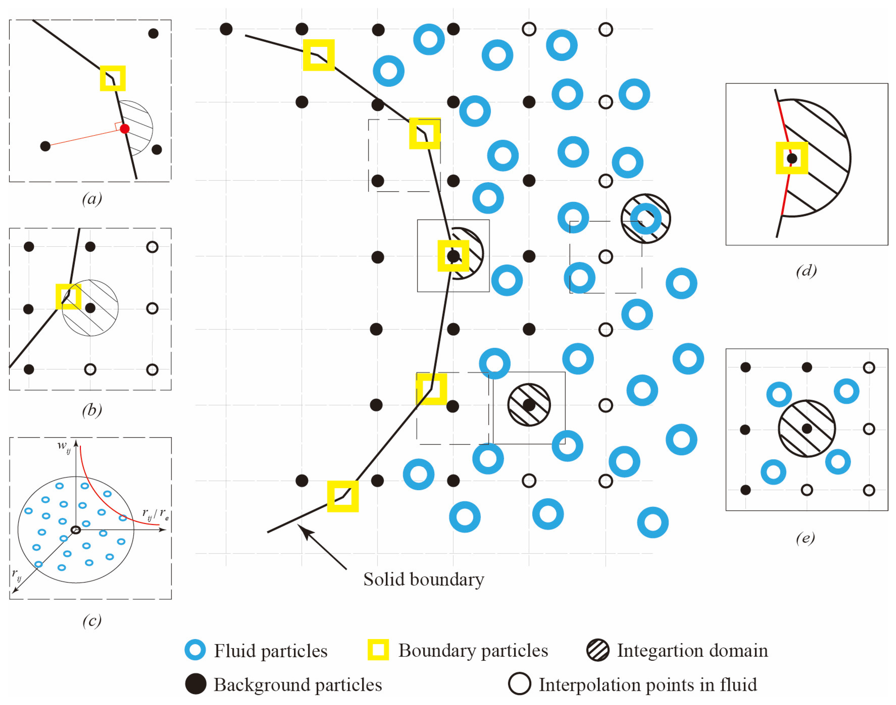
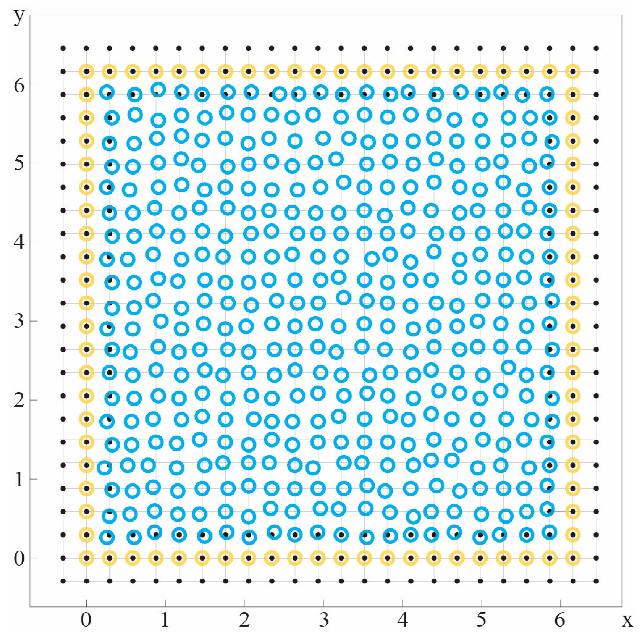
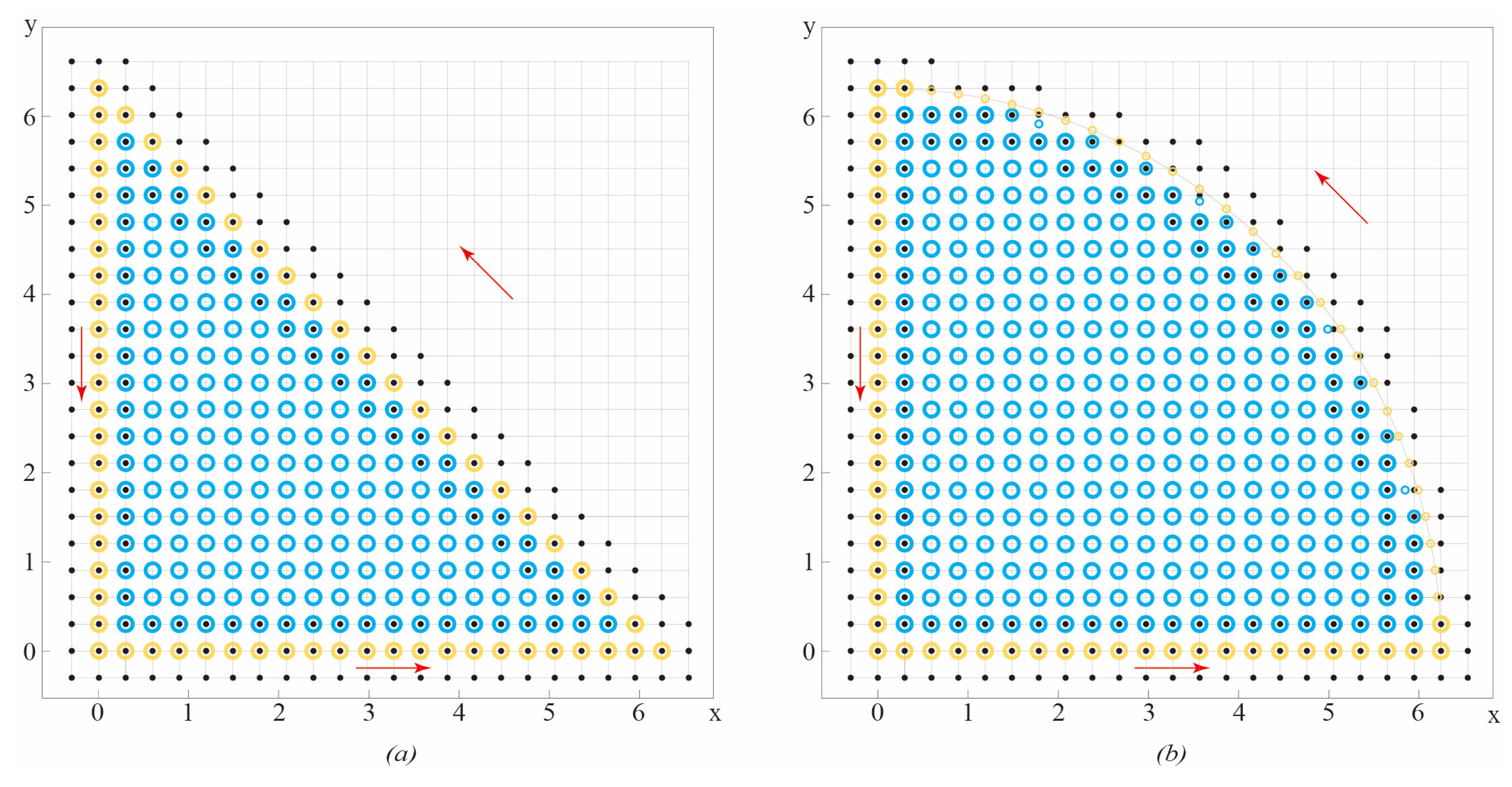
2.2. Enhancing the Boundary Condition Accuracy by Local Regular-Distributed Particles

The insufficiency of the support domain for the particles close to the boundaries is the main source of the difficulty in enforcing accurate boundary conditions in the particle methods. As discussed in the Introduction section, various techniques have been proposed based on the idea of adding additional layers of particles outside the boundary, such as the virtual particle method and the mirror particle method [11,16]. But, this type of technique usually needs artificial parameters that must be tuned for different problems. More importantly, the additional layers make it difficult to accommodate cases with complex geometries.
In order to fundamentally address the issues related to the insufficiency of the support domain while still preserving the meshless nature of the method, a new approach is adopted. This approach (as shown in Figure 1) involves establishing an area with regular-distributed particles across the boundaries, where the field variables on the particles (i.e., pressure in this paper) are treated as new unknowns in solving the Poisson equation. In order to distinguish from the original fluid and solid particles, these newly added particles are called background particles in this paper.
This new local regular-distributed background particles (LRBP) method aims to solve the problem of insufficient particles in the support domain when the fluid particles are close to the boundary. The core idea of the method is to establish a regular-distributed background particle area near the boundary and use the new unknown variable (pressure in this paper) carried by the background particles for spatial discretization. By performing Poisson equation calculations for each background particle, a new system of equations is introduced to solve these new unknown variables. When the fluid particles are within the background particle area, the unknown variables can be indirectly involved in the calculation by weighted summation from nearby background particles rather than directly solving the Poisson equation. For fluid particles in the internal flow domain, the boundary issues will not affect them and, therefore, they can be calculated according to the usual methods used in particle methods such as ISPH and MPS.
This separation of boundary/near-boundary and inner particles makes this method easier to implement in particle method algorithms. Unlike the traditional virtual particle method and the mirror particle method, this method does not need to adapt to boundary shapes and can directly impose boundary conditions on boundary particles without artificial maintenance.
The remaining questions of implementing this new framework include how to efficiently impose boundary conditions on boundary particles, how to solve new unknown variables, and how to accurately interpolate between background particles and fluid particles within the domain.
For the first question, it is recommended to use a weak form scheme to handle the boundary conditions, which makes it easier to impose boundary conditions on boundary particles, especially for Neumann boundary conditions.
For the second question, it is suggested to introduce new equations near the boundary and its vicinity, such as points between neighboring solid boundary particles, and impose boundary conditions on them. This will naturally introduce these new unknown variables into the equation system and make the equation system more representative of the real situation.
For the last question, it is suggested to use a least squares-type interpolation method in the background region, while conventional ISPH or MPS-type interpolation methods can be used in the internal region. This can achieve accurate interpolation and improve the accuracy and efficiency of the particle methods.
The details of these three key parts in the new framework will be discussed in the following sections of this paper.

2.3. Weak Form Poisson Equation and Imposing Boundary Condition

Assuming a finite region Ω with an arbitrary boundary Γ , integrating over Ω after multiplying Equation (1) by an arbitrary test function ϕ yields the following relationship:
Ω 2 p b ϕ d Ω = 0 ,
which is chosen appropriately to satisfy p 2 ϕ = 0 , and then the above equation can be further written using Gauss’s formula:
Γ n ϕ p n p ϕ d S = Ω b ϕ d Ω ,
where Γ is the integral along the boundary Γ , d Ω denotes the area element on Ω , d S denotes the length element on Γ , and n is the unit normal vector on the boundary.
Further organization leads to the Poisson equation of an integral type in the form of
Γ p n ϕ d Γ Ω p ϕ d Ω = Ω b ϕ d Ω .
In solving practical problems, Poisson’s equation can be solved by various numerical or analytical methods depending on the specific boundary conditions and the integration region. For example, the Heaviside step function is chosen as the test function, so the weakly compressible integral Poisson equation can be expressed as:
Γ p n ϕ d Γ = Ω b ϕ d Ω .
In the framework of the weakly compressible integral Poisson described above, the Neumann boundary condition can be easily imposed, thus guaranteeing the consistency of the whole system of linear equations.
As shown in Figure 1d, when applying boundary conditions on the boundary particles, the integration domain is a sector region enclosed by the boundary lines. The distribution function is composed of the known boundary conditions (red lines), the arc of a circle (black line), and the function over the sector surface area. Therefore, in this case, the left-hand side integral of Equation (6) is composed of two parts: the line integrals along the known boundary conditions and the arc. The right-hand side integral represents the double integration of the source term of the Poisson equation over the sector surface area. In Figure 1e, where the background particle is integrated within the complete integration domain, the corresponding integrals of Equation (6) can be directly computed.

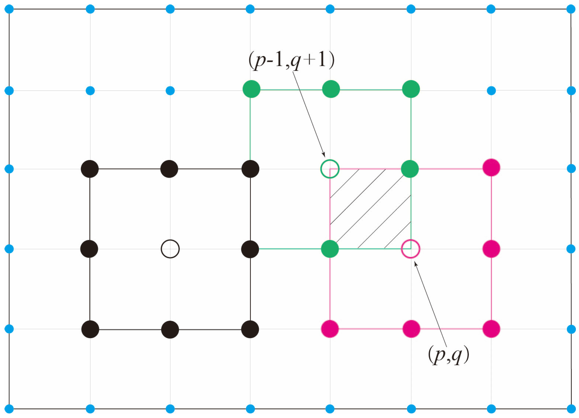
2.4. Closure Equations for the Background Particles

2.4.1. Closure Equations for Different Parts of Background Particles

As mentioned in Section 2.2, when solving the Poisson equation, the pressure variables on the background particles are treated as new unknowns, resulting in an overdetermined system of linear equations. Therefore, it is necessary to enforce the computation of the Poisson equation on the background particles, as given by Equation (6), in order to establish equations at the locations of the new unknown variables. Based on the distribution of the background particles, they can be classified into four categories: outside the boundary, closest to the boundary particles (or on the boundary), inside the background region, and closest to the fluid particles.
When discretizing the continuous boundary, the positions of the boundary particles can be represented using background particles on the left and right sides. This means that complex boundary shapes can also be easily represented. For background particles outside the boundary (as shown in Figure 1a), the nearest point on the boundary (red point) can be found, and a new Poisson equation can be introduced with this point as the center. For background particles inside the computational domain and closest to the boundary (Figure 1b), the physical information they carry can be understood as the value of the field variable at a certain point in time. Therefore, the Poisson equation can be directly written for these particles. The same treatment applies to background particles inside the background region. When it comes to the background particles closest to the fluid particles, i.e., Figure 1c, there are sufficient fluid particles in their support domain, which allows the Poisson equation to be solved according to the ISPH and MPS methods.
In the proposed local regular-distributed particles scheme, when discretizing the operators on the background region, the smallest shape function construction unit is the 9-point grid formed by the current computing point and its surrounding 8 points. This ensures that all the unknowns of the background particles are included in the equations and not overlooked. However, it is important to note that when evaluating Equation (6) on the boundary discretized points and background particles near the boundary, the integration regions should avoid overlapping as much as possible to avoid calculation errors.
The following Section 2.5 will describe in detail the construction method of the shape functions, i.e., how to obtain the expression of the current unit’s function using the 9 unknowns of the minimal interpolation function unit, as shown in Figure 2.

2.4.2. Gauss–Legendre Quadrature Formula

In the framework of the aforementioned weak-form integral equation, the choice of an appropriate integration method is equally important. The Gauss–Legendre integration method is a commonly used numerical integration method that offers high accuracy and good stability compared to other numerical integration methods. Moreover, it exhibits good adaptability in handling various types of functions, including high-order polynomials.
The Gauss–Legendre quadrature formula is an implementation within the framework of Gauss-type quadrature formulas, with specific interpolation nodes and weight coefficients. In computing the sampling points and weights, the Gauss–Legendre quadrature formula utilizes the properties of Legendre polynomials to enhance the accuracy of numerical integration, where the quadrature points are the zeros of Legendre polynomials and the interval is [ 1 , 1 ] . Therefore, for the Gauss–Legendre quadrature formula on a general bounded integration interval [ a , b ] , a simple transformation can be made by setting x = b a 2 t + b + a 2 , which yields the following equation [19,20]:
I = b a 2 1 1 f b a 2 t + b + a 2 d t b a 2 i = 0 n A i f ( b a 2 t i + b + a 2 ) ,
where A i and t i are the weights and Gaussian points on the interval [ 1 , 1 ] .
In a similar manner, the expression of the double Gauss–Legendre quadrature formula is
I = 1 1 d x 1 1 f x , y d y k = 0 m l = 0 n A k l f x k , y l .
Furthermore, the expression on the general integration interval can be obtained through a change of interval, which yields
I = a b d x c d f x , y d y = b a d c 4 1 1 d s 1 1 f b a 2 s + b + a 2 , d c 2 t + d + c 2 d t , = J a c i = 1 n j = 1 n A i A j f x s i , y t j
where s i and t j are the Gaussian points, A i and A j are the weights, and J a c is the Jacobian transformation coefficient.
Therefore, the aforementioned Equation (7) can be used to compute the left-hand term of Equation (6), while Equation (9) can be used to compute the right-hand term.

2.5. Different Interpolation Techniques

As mentioned above, obtaining the gradient operator and Laplace operator of pressure is also an important step. In the meshless methods, there are already many numerical models available for the gradient and Laplace operators. Additionally, first-order and second-order derivatives can be obtained by constructing the expression of the pressure function.

2.5.1. Least Square Type Interpolation Based on Taylor Series Expansion

For a differentiable function f x , y , the second-order Taylor series expansion at a given point p x 0 , y 0 has the following general form [21]:
f ( x , y ) f ( x 0 , y 0 ) + ( x x 0 ) f x | p + ( y y 0 ) f y | p + 1 2 ( x x 0 ) 2 2 f x 2 | p + ( x x 0 ) ( y y 0 ) 2 f x y | p + 1 2 ( y y 0 ) 2 2 f y 2 | p
and for convenience of expression, it can be abbreviated as
f ( x , y ) = f 0 + h f x 0 + k f y 0 + 1 2 h 2 f x x 0 + h k f x y 0 + 1 2 k 2 f y y 0 ,
where h = x x 0 , k = y y 0 , f 0 = f x 0 , y 0 , f x 0 = f x ( x 0 , y 0 ) , f y 0 = f y ( x 0 , y 0 ) , f x x 0 = f x x x 0 , y 0 , f x y 0 = f x y x 0 , y 0 , f y y 0 = f y y x 0 , y 0 .
If there are sufficient neighboring points j ( j = 1 , 2 , N ) within the support domain of point p , and the function values f j = f x j , y j are known, the expression of the derivatives of various orders at point p can be approximated by solving a series of linear equations. The series of linear equations can be written in matrix form, as follows:
A D f f = 0 ,
i.e.,
h 1 k 1 1 2 h 1 2 h 1 k 1 1 2 k 1 2 h 2 k 2 1 2 h 2 2 h 2 k 2 1 2 k 2 2 h N k N 1 2 h N 2 h N k N 1 2 k N 2 f x 0 f y 0 f x x 0 f x y 0 f y y 0 = f 1 f 0 f 2 f 0 f N f 0 .
From the above equation, it can be seen that the desired derivatives of various orders are the unknowns. Therefore, in order to solve the above linear equations, there should be at least 5 neighboring points to the point p . To improve the accuracy of the approximation, more than 5 points should be used. However, this will lead to the linear equations being overdetermined. Therefore, according to the least squares method, a weight function w r is introduced, and the following standard error criterion E is defined:
E = j = 1 N f 0 f j + h j f x 0 + k j f y 0 + 1 2 h j 2 f x x 0 + h j k j f x y 0 + 1 2 k j 2 f y y 0 w j 2 ,
where w r is the weighted function in the least squares method, and here it is common to use the singular weight function in the MPS method.
w ( R , d r ) = R d r 1 0 d r R 0 R d r
When E D f = 0 , the standard error is minimized and, thus, a set of five equations with five unknowns is obtained, the solving of which leads to the unknown derivatives.
A = w j 2 h j 2 w j 2 h j k j w j 2 1 2 h j 2 w j 2 h j 2 k j w j 2 1 2 h j k j 2 w j 2 h j k j w j 2 k j 2 w j 2 1 2 h j 2 k j w j 2 h j k j 2 w j 2 1 2 k j 3 w j 2 1 2 h j 3 w j 2 1 2 h j 2 k j w j 2 1 4 h j 4 w j 2 1 2 h j 3 k j w j 2 1 4 h j 2 k j 2 w j 2 h j 2 k j w j 2 h j k j 2 w j 2 1 2 h j 3 k j w j 2 h j 2 k j 2 w j 2 1 2 h j k j 3 w j 2 1 2 h j k j 2 w j 2 1 2 k j 3 w j 2 1 4 h j 2 k j 2 w j 2 1 2 h j k j 3 w j 2 1 4 k j 4 ,
D f = f x 0 f y 0 f x x 0 f x y 0 f y y 0 ,   f = f j w j 2 h j f 0 w j 2 h j f j w j 2 k j f 0 w j 2 k j f j w j 2 h j 2 2 f 0 w j 2 h j 2 2 f j w j 2 h j k j f 0 w j 2 h j k j f j w j 2 k j 2 2 f 0 w j 2 k j 2 2 .

2.5.2. Moving Particle Semi-Implicit Method (MPS)

The MPS (Moving Particle Semi-implicit) method, which was first introduced in the work of Koshizuka and Oka [11], is a meshless numerical method that simplifies the computation process by using a simplified continuity equation to solve the fluid motion equations. Compared to SPH, the MPS method improves the stability and accuracy of numerical solutions by introducing a semi-implicit handling technique. The implicit treatment enables the numerical solution to be less sensitive to the choice of time step, thus allowing for the use of larger time steps. The pressure field of the MPS method is obtained by solving the pressure Poisson equation using a semi-implicit approach instead of using the equation of state as in the SPH method.
In addition, the discretization of operators in the MPS method is different from that in the SPH method. In the MPS method, the gradient operator discretizes the particle interaction forces based on mathematical concepts, associating them with velocity and density. Its role is to discretize the pressure gradient using the distances between particles and the weights of the kernel function. By summing the weighted gradients of all the particles within the support domain of a particle, the gradient operator can be obtained.
ϕ i = d n 0 j i ϕ j ϕ i r j r i 2 r j r i w r j r i ,
where d is the number of spatial dimensions, n 0 is the initial particle number density, ϕ is the physical quantity, r is the coordinate, and w ( r ) is the kernel function.
w r = r e r 1 0 r r e 0 r e r
The Laplacian operator in the MPS method is analogous to a second-order derivative. By considering the function values and positions of neighboring particles, the Laplace operator incorporates the interaction effects between particles into the discretized computation model. Initially, the Laplace operator in MPS was derived from linear diffusion problems, where the Laplace operator of a variable is considered equivalent to the temporal diffusion of that variable. The diffusion of particles is constrained within the support domain of the kernel function, and the Gaussian function is replaced by the kernel function to obtain the increment of the physical quantity within a Δ t time step.
Since diffusion is a linear problem, the transport of a physical quantity ϕ between particles and neighboring particles in time can be weighted and superimposed. Additionally, the diffusion problem of a physical quantity ϕ in the time domain can be regarded as a Laplacian method. Therefore, the Laplacian operator model is as follows:
2 ϕ i = 2 d n 0 λ j i ϕ j ϕ i w r j r i ,
where λ is the compensation for the error introduced by replacing the Gaussian function with a kernel function.
λ = j i w r j r i r j r i 2 j i w r j r i

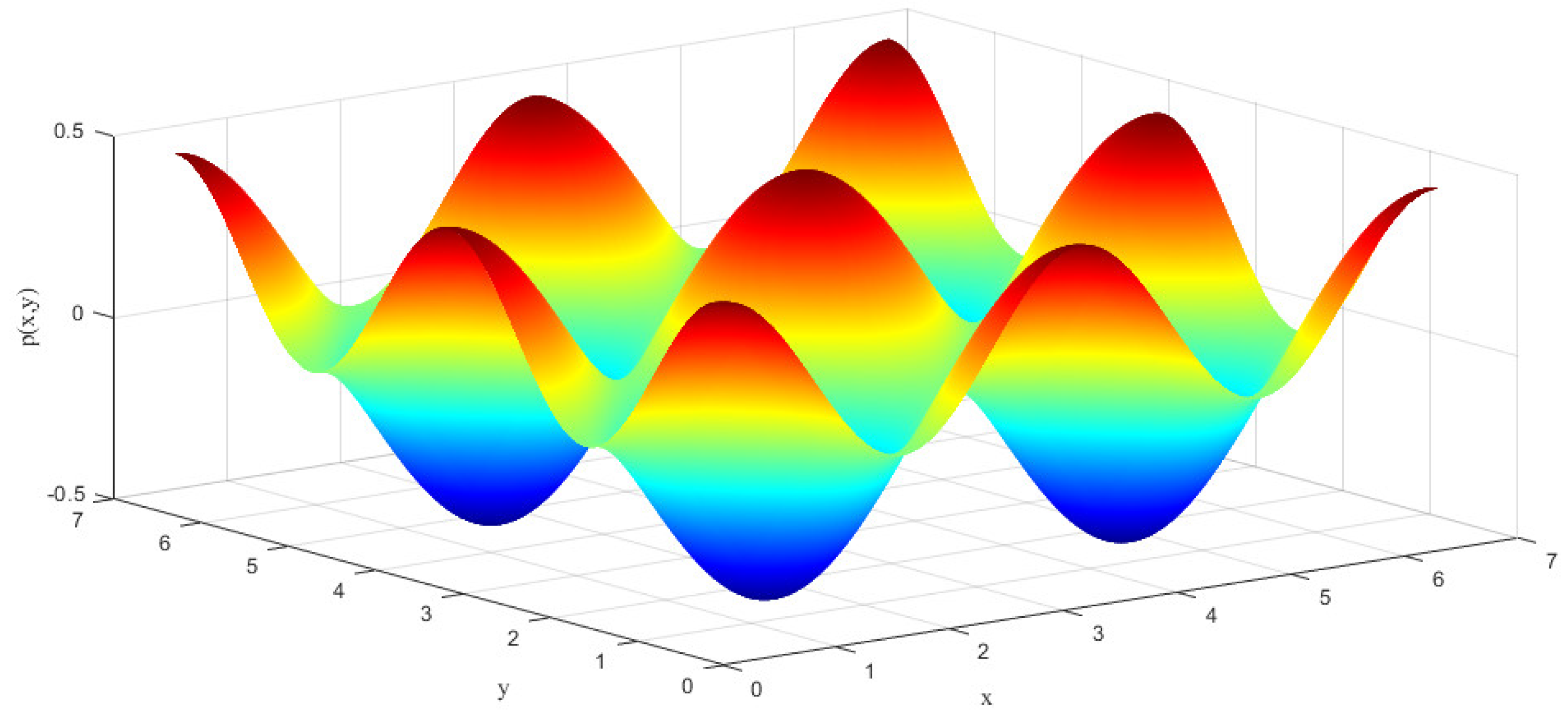
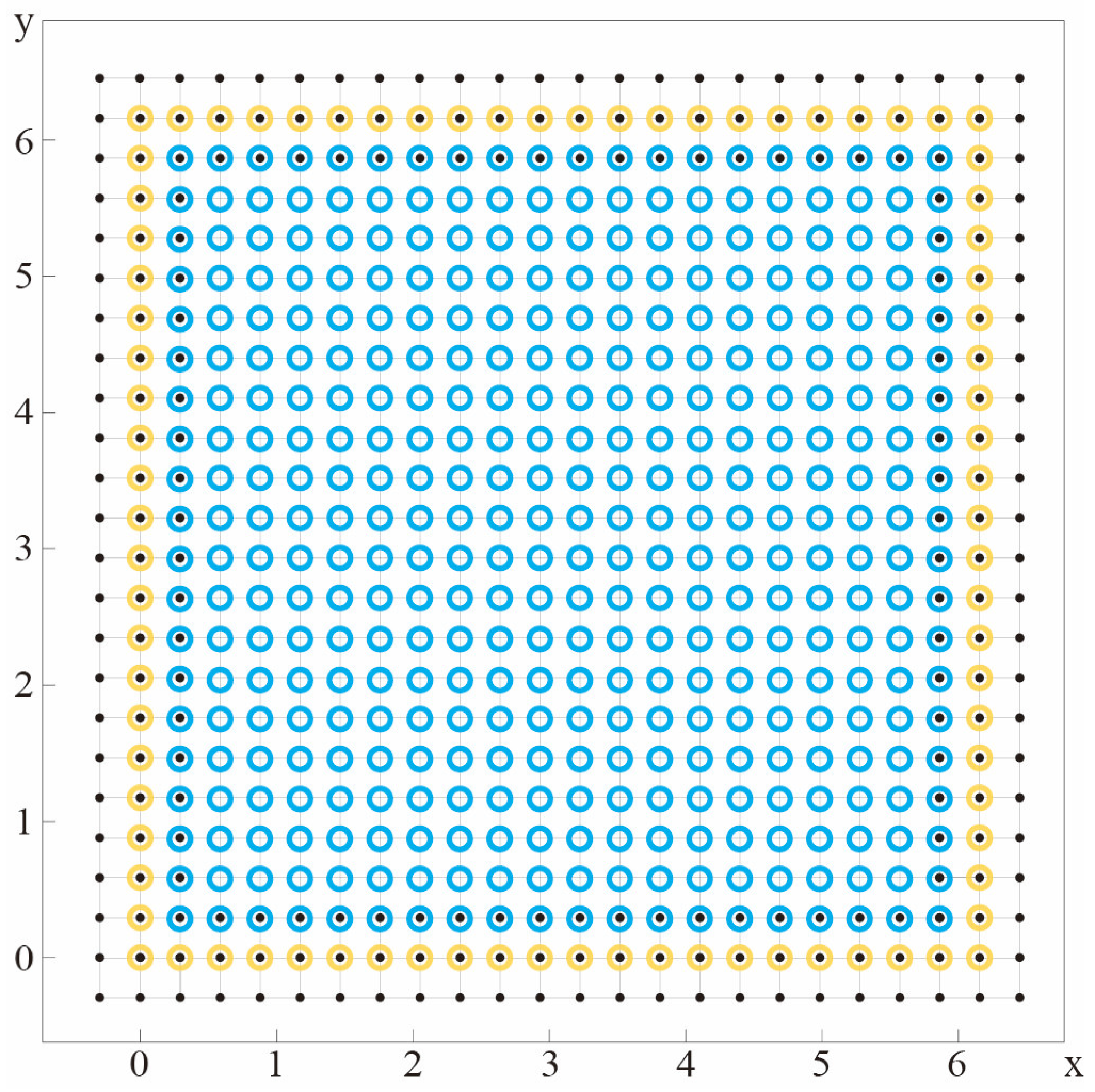
3. Numerical Results and Discussion

To demonstrate the accuracy and efficiency of the proposed algorithm for solving the Poisson equation, the Taylor–Green vortex [22] is chosen as an example for numerical validation.
The Taylor–Green vortex is a classic fluid dynamics problem that describes a rotating vortex in a two-dimensional plane. In this problem, the initial velocity distribution of the vortex satisfies the two-dimensional, steady, incompressible Navier–Stokes equations, and the velocity and pressure fields of the vortex satisfy the Poisson equation, i.e., Equation (22), at a given time t = t p .
2 p x , y = 2 ρ v x x , y u y x , y u x x , y v y x , y ,
where p is the pressure, ρ is the fluid density, and the subscripts x and y refer to partial derivatives with respect to x and y , respectively.
The initial velocity distribution of the Taylor–Green vortex can be represented by a simple mathematical function, Equations (23) and (24), commonly known as the Green function. This function takes the form of a mathematically defined rotating rule, which allows the fluid to form a vortex at the initial moment. The vortex continues to rotate and deform in a certain pattern over time.
u ( x , y , t ) = U 1 e 2 π 2 ξ sin ( 2 π x ) cos ( 2 π y ) ,
v ( x , y , t ) = U 1 e 2 π 2 ξ cos ( 2 π x ) sin ( 2 π y ) ,
where U is the velocity, u and v are the components of velocity vector, ξ = t T is dimensionless time, υ is the kinematic viscosity coefficient, and T is a parameter defining the angular velocity of the vortex.
The Taylor–Green vortex has significant applications, particularly in fluid dynamics and turbulence research. It is widely used to verify the accuracy and efficiency of numerical algorithms, as it has a known analytical solution, and the evolution of the vortex can be simulated numerically. By comparing the numerical results of an algorithm with the analytical solution, we can assess the performance and accuracy of the algorithm.
In this analysis, the computational domain is set to 0 , 2 π × 0 , 2 π , and the initial velocity field is given as [23]:
u x , y , t = sin x cos y e 2 υ t ,
v x , y , t = cos x sin y e 2 υ t ,
where ρ = 1 , υ = 1   m 2 / s , and t = 10 4   s are selected. The pressure field of the Taylor–Green vortex is shown in Figure 3.

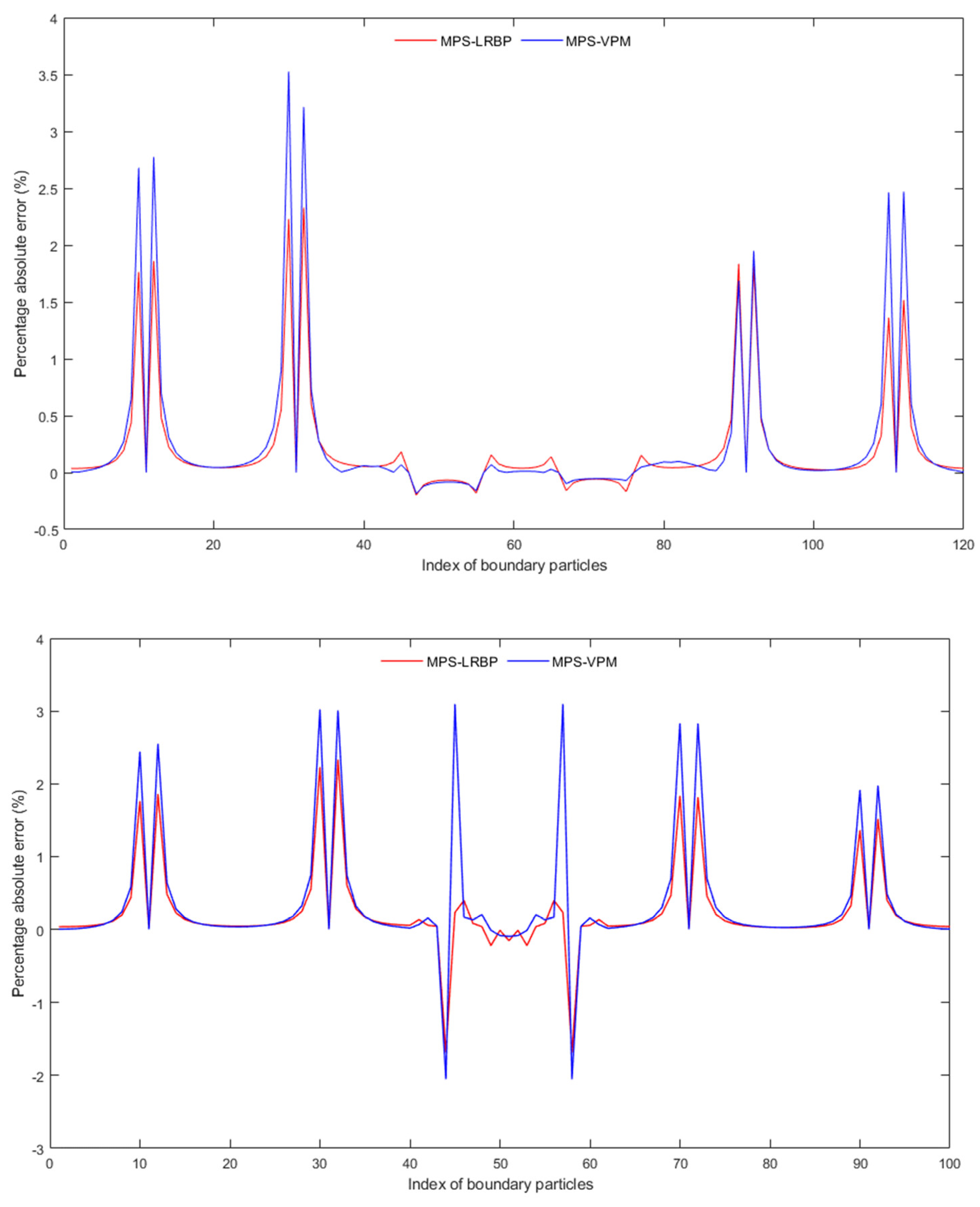
3.1. Validation of Boundary Local Background Particles Method

To verify the effectiveness and accuracy of introducing the background particles as a replacement for the virtual particle method, a set of different grid sizes is selected to calculate the pressure field of the Taylor–Green vortex under Neumann boundary conditions, which refers to the normal derivative of vorticity being zero at the boundary of the vortices:
p x ( 0 , y ) = p x ( 2 π , y ) = ρ 4 cos 2 y e 2 υ t p 2 ,
p y ( x , 0 ) = p y ( x , 2 π ) = ρ 4 cos 2 x e 2 υ t p 2 ,
and an example of the grid points in the domain is shown in Figure 4.
In the case of regular particle distribution, calculations are performed by combining the LRBP method with the MPS method and the least square-type interpolation method separately. As shown in Table 1, LS represents the combination of the Least Squares interpolation, MPS-LRBP represents the combination of the MPS method and the LRBP method, while MPS-VPM represents the combination of the MPS method and the virtual particle method. To better evaluate the accuracy of solving the Poisson equation by the combination of the interpolation functions construction and background particles scheme, the L 2 norm and L norm are introduced for statistical analysis. The variations of the errors with the grid size are plotted to investigate the convergence order of the proposed interpolation method.
E r r L 2 = u n u m u a n 2 u a n 2 ,
E r r L = u n u m u a n u a n ,
where u n u m and u a n are the numerical and analytical solutions, respectively.
As shown in the convergence curves of Figure 5, with an increase in the particle numbers, the convergence rate of the overall pressure field of the least square-type interpolation method combined with the LRBP method tends to be around 3, and the convergence rate fluctuates little at different initial particle spacings, basically stabilizing around 2.6. The convergence rate of the MPS method combined with the LRBP is slightly lower, and the convergence rate fluctuates at different initial particle spacings. However, from the trend of its convergence curve, it can be seen that its overall convergence rate is around 2.5, which is still an acceptable and good result. To better demonstrate the accuracy of the LRBP method, the convergence of the original MPS method combined with VPM (virtual particle method) is calculated, and the result is as expected, that is, the convergence rate tended to be 1. Therefore, the LRBP method has good numerical accuracy and can be well applied in practical computing.

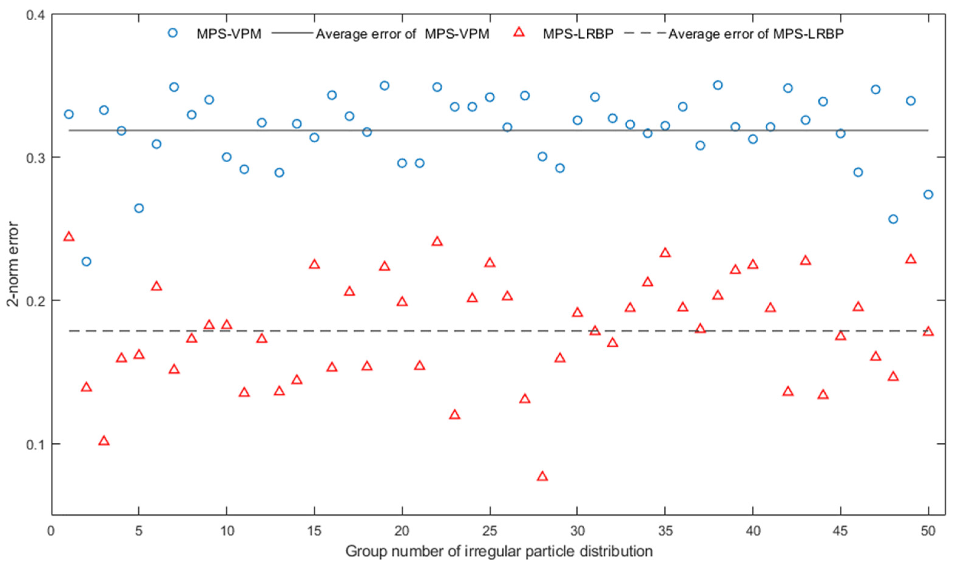
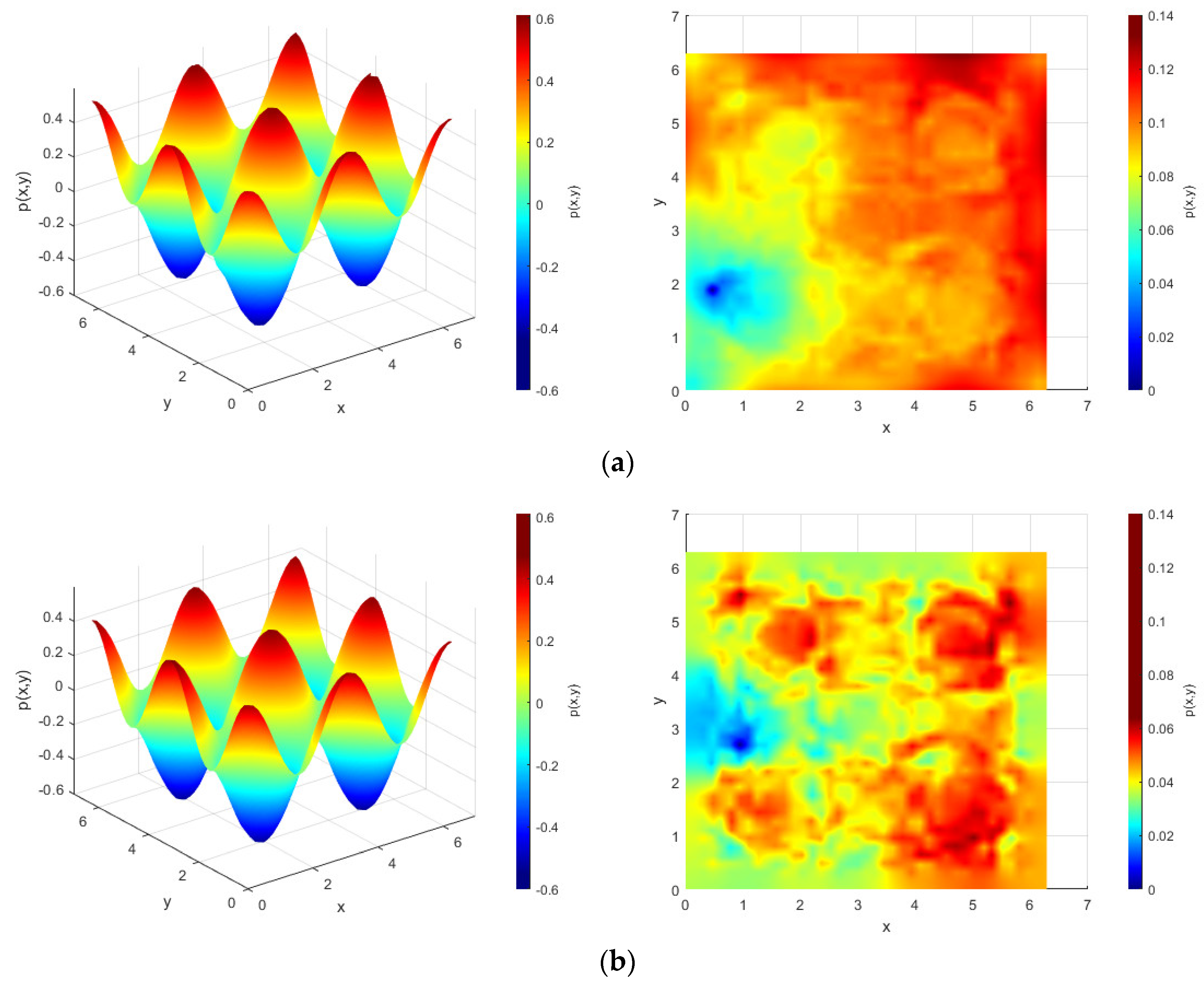
3.2. Different Choice of Interpolation Methods for Inner Areas

The difference in the size of the influence radius and particle search radius, as well as the distinct interpolation principles of the two, implies a high degree of flexibility in the proposed algorithm. When using local background particles instead of placing virtual particles, different gradient operators and Laplacian models can be used to calculate the Poisson equation for the particles in the fluid. Next, the coupled calculation with the MPS method, which is widely used and has sufficient development, will be performed to verify the compatibility and flexibility of the algorithm.
Due to the flow motion, the particles are not uniformly distributed in space, which makes it necessary to verify the accuracy of calculations for irregularly distributed points. As shown in Figure 6, an irregular particle distribution is obtained by applying random noise to the internal fluid particle points within the computational domain. The parameters selected in this section are the initial distance d r = π / 20 and the support domain radius r e = 2.1 d r . The random noise is defined as a uniform distribution within a radius of 0.1 d r around the original position of the 41 × 41 regular grid. The randomization process is repeated to generate 50 groups of irregular distribution.
Based on the 2-norm, error statistics are performed on the numerical solution of the Taylor–Green vortex. In 50 sets of non-repeating and irregular initial particle distributions, as shown in Figure 7, the global 2-norm error combined with the LRBP method is lower, with a fluctuation range of 0.05–0.25 and an average 2-norm error of about 0.18. In contrast, the 2-norm error range with the virtual particle method is between 0.27 and 0.35, with an average 2-norm error of about 0.32. Therefore, combining the LRBP method results in smaller calculation errors and higher accuracy. In order to analyze the pressure field more intuitively, a pressure field cloud map and an absolute error cloud map are given for a certain particle distribution. From Figure 8, it can be seen that the virtual particle method has lower accuracy in solving the boundary and slightly larger errors in the entire pressure field, while the LRBP method has improved accuracy in solving the boundary pressure values and also improved the calculation of the internal pressure field. This proves that combining the LRBP method with the MPS method for calculation is feasible and can improve the calculation accuracy to a certain extent.

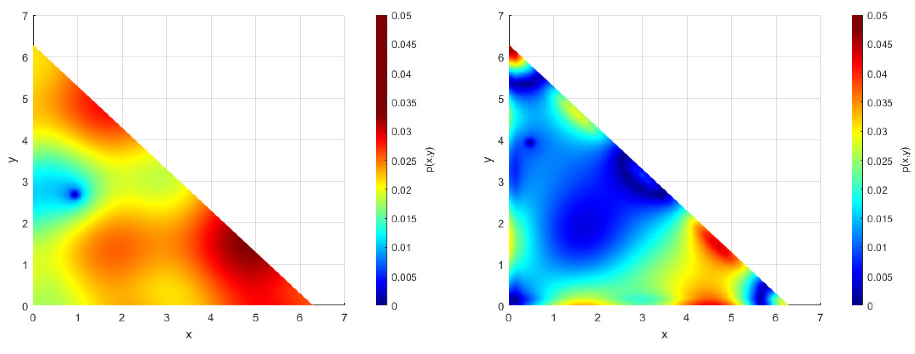
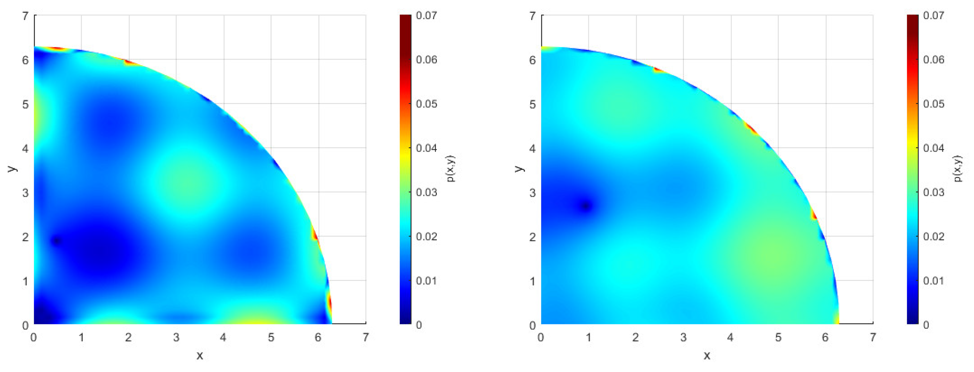
3.3. Different Shapes for the Boundary

To further explore the effectiveness of the background particle method in dealing with problems with complex boundary shapes, the shape of the computational domain is changed based on the previous problem. Two boundary conditions are selected: a triangular boundary and a quarter-circle boundary.
Based on the previous section, it is known that the error is smaller when combining the background particle method with the MPS method. Therefore, the background particle method is used at the boundary and the MPS method is used internally. The particles are evenly distributed and the initial particle spacing for the calculation is d r = π / 20 , where the support domain radius is 2.1 d r . The particle distribution is shown in Figure 9.
To visually analyze the accuracy of the background particle method in calculating the boundary pressure values, the numerical solution of the boundary particles is compared to the theoretical solution in Figure 10 and Figure 11, according to the numbering order of the boundary particles in the direction of the arrows in Figure 9. For the triangular boundary, it can be seen that the computational accuracy is consistent, and the error is small on the boundary. For the quarter-circle boundary, the error is smaller on the straight boundary compared to the curved boundary, which is due to the discrete nature of the boundary particles affecting the calculation. At the same time, it can be seen from the error cloud map that combining the LRBP method improves the accuracy of calculating the boundary pressure values and is more accurate in solving the internal flow field than using the virtual particle method, and its error fluctuation range is also smaller. It can be concluded that the background particle method can effectively handle these types of boundary problems and has the potential to handle problems with complex boundary shapes.

4. Conclusions

This article proposes a new boundary handling scheme called Local Regular Distribution Background Particles (LRBP), which retains the meshless characteristics of most domains while solving problems such as insufficient particles in the local support domain of traditional boundary handling methods and difficulty in representing complex boundaries. Compared to the commonly used virtual particle method (VPM), as a new approach for boundary handling, this scheme avoids the placement of virtual particles through background particles, making it easier to represent different boundary shapes and apply boundary conditions. In addition, information transfer between fluid particles and boundary particles is achieved by background particles delved into the fluid domain. To validate the numerical accuracy and ability to handle complex boundary problems of the proposed LRBP method and the commonly used virtual particle method, the popular MPS method is used for verification. The boundary handling methods are selected by the LRBP method and the virtual particle method, respectively. The comparison is conducted using the Taylor–Green vortex, and the results show that the proposed LRBP method has a third-order convergence accuracy, which is significantly higher than the first-order accuracy of the MPS method. Furthermore, under irregular particle distributions, the coupled LRBP method has a higher flow field solution accuracy than the coupled virtual particle method, especially at the boundary. Additionally, calculations with complex solid boundaries show that the LRBP method has better accuracy than the virtual particle method and can handle such problems well. Due to its higher numerical accuracy, applicability, and ability to handle complex boundary problems, the LRBP method as a new boundary-handling approach has great potential for application. Currently, LRBP-related work mainly focuses on its feasibility, accuracy, and applicability, and in future research, it will be necessary to apply the LRBP method to actual flow problems for further testing. In addition to applying the LRBP method to solid boundary conditions, the local regular-distributed background particles can also serve as a medium for information transfer. Therefore, its application to structural interaction and fluid–structure interaction problems is also a potential area for future research.

Author Contributions

Conceptualization, Z.S., L.D., Z.M., S.T., Z.Z., K.D. and G.Z.; investigation, Z.S., L.D. and S.T.; resources, Z.S.; data curation, L.D. and S.T.; writing—original draft preparation, Z.S., L.D. and S.T.; writing—review and editing, Z.M., Z.Z., K.D. and G.Z.; supervision, Z.S.; project administration, Z.S.; funding acquisition, Z.S. All authors have read and agreed to the published version of the manuscript.

Funding

This work is supported by the National Key Research and Development Program of China (2021YFC2801701 & 2021YFC2801700), the National Natural Science Foundation of China (No. 52171295, 52192692), and Fundamental Research Funds for the Central Universities (No. DUT22LK17).

Institutional Review Board Statement

Not applicable.

Informed Consent Statement

Not applicable.

Data Availability Statement

All data have been provided in this paper. Further inquiries can be directed to the corresponding authors.

Acknowledgments

Many thanks to the funders, as well as all the authors for their hard work and dedication.

Conflicts of Interest

Author Zongbao Mu was employed by the company Dalian Ship building Industry Company. The remaining authors declare that the research was conducted in the absence of any commercial or financial relationships that could be construed as a potential conflict of interest.

References

  1. Sun, Z.; Liu, G.; Zou, L.; Zheng, H.; Djidjeli, K. Investigation of Non-Linear Ship Hydroelasticity by CFD-FEM Coupling Method. J. Mar. Sci. Eng. 2021, 9, 511. [Google Scholar] [CrossRef]
  2. Zhang, G.; Hu, T.; Sun, Z.; Wang, S.; Shi, S.; Zhang, Z. A delta SPH-SPIM coupled method for fluid-structure interaction problems. J. Fluid Struct. 2021, 101, 103210. [Google Scholar] [CrossRef]
  3. Kim, K.S.; Kim, M.H.; Park, J. Development of Moving Particle Simulation Method for Multiliquid-Layer Sloshing. Math. Probl. Eng. 2014, 2014, 350165. [Google Scholar] [CrossRef]
  4. Sun, Z.; Djidjeli, K.; Xing, J.T.; Cheng, F. Coupled MPS-modal superposition method for 2D nonlinear fluid-structure interaction problems with free surface. J. Fluid Struct. 2016, 61, 295–323. [Google Scholar] [CrossRef]
  5. Khayyer, A.; Gotoh, H. A Multiphase Compressible-Incompressible Particle Method for Water Slamming. Int. J. Offshore Polar 2016, 26, 20–25. [Google Scholar] [CrossRef]
  6. Chaudhry, A.Z.; Shi, Y.; Pan, G. Recent developments on the water entry impact of wedges and projectiles. Ships Offshore Struct. 2022, 17, 695–714. [Google Scholar] [CrossRef]
  7. Sun, Z.; Djidjeli, K.; Xing, J.T. The weak coupling between MPS and BEM for wave structure interaction simulation. Eng. Anal. Bound. Elem. 2017, 82, 111–118. [Google Scholar] [CrossRef]
  8. Khayyer, A.; Tsuruta, N.; Shimizu, Y.; Gotoh, H. Multi-resolution MPS for incompressible fluid-elastic structure interactions in ocean engineering. Appl. Ocean Res. 2019, 82, 397–414. [Google Scholar] [CrossRef]
  9. Hwang, S.; Khayyer, A.; Gotoh, H.; Park, J. Development of a fully Lagrangian MPS-based coupled method for simulation of fluid-structure interaction problems. J. Fluid Struct. 2014, 50, 497–511. [Google Scholar] [CrossRef]
  10. Shao, S.; Lo, E.Y.M. Incompressible SPH method for simulating Newtonian and non-Newtonian flows with a free surface. Adv. Water Resour. 2003, 26, 787–800. [Google Scholar] [CrossRef]
  11. Koshizuka, S.; Oka, Y. Moving-particle semi-implicit method for fragmentation of incompressible fluid. Nucl. Sci. Eng. 1996, 123, 421–434. [Google Scholar] [CrossRef]
  12. Solenthaler, B.; Pajarola, R. Predictive-Corrective Incompressible SPH. ACM T Graph. 2009, 28, 1–6. [Google Scholar] [CrossRef]
  13. Ihmsen, M.; Cornelis, J.; Solenthaler, B.; Horvath, C.; Teschner, M. Implicit Incompressible SPH. IEEE Trans. Vis. Comput. Graph. 2014, 20, 426–435. [Google Scholar] [CrossRef] [PubMed]
  14. Nomeritae, N.; Bui, H.H.; Daly, E. Modeling Transitions between Free Surface and Pressurized Flow with Smoothed Particle Hydrodynamics. J. Hydraul. Eng. 2018, 144, 4018012. [Google Scholar] [CrossRef]
  15. Monaghan, J.J. Simulating free-Surface flows with sph. J. Comput. Phys. 1994, 110, 399–406. [Google Scholar] [CrossRef]
  16. Xie, H.; Koshizuka, S.; Oka, Y. Modelling of a single drop impact onto liquid film using particle method. Int. J. Numer. Methods Fluids 2004, 45, 1009–1023. [Google Scholar] [CrossRef]
  17. Monaghan, J.J.; Kajtar, J.B. SPH particle boundary forces for arbitrary boundaries. Comput. Phys. Commun. 2009, 180, 1811–1820. [Google Scholar] [CrossRef]
  18. Park, S.; Jeun, G. Coupling of rigid body dynamics and moving particle semi-implicit method for simulating isothermal multi-phase fluid interactions. Comput. Method Appl. M 2011, 200, 130–140. [Google Scholar] [CrossRef]
  19. Shivaram, K.T. Gauss Legendre quadrature over a unit circle. Int. J. Eng. Tech. Res. 2013, 2, 1043–1047. [Google Scholar]
  20. Shivaram, K.T. Generalised Gaussian Quadrature over a Sphere. Int. J. Sci. Eng. Res. 2013, 4, 1530–1534. [Google Scholar]
  21. Koh, C.G.; Gao, M.; Luo, C. A new particle method for simulation of incompressible free surface flow problems. Int. J. Numer. Methods Eng. 2012, 89, 1582–1604. [Google Scholar] [CrossRef]
  22. Taylor, G.I.; Green, A.E. Mechanism of the Production of Small Eddies from Large Ones. Proc. R. Soc. Lond. Ser. A Math. Phys. Sci. 1937, 158, 499–521. [Google Scholar]
  23. Bardazzi, A.; Lugni, C.; Antuono, M.; Graziani, G.; Faltinsen, O.M. Generalized HPC method for the Poisson equation. J. Comput. Phys. 2015, 299, 630–648. [Google Scholar] [CrossRef]
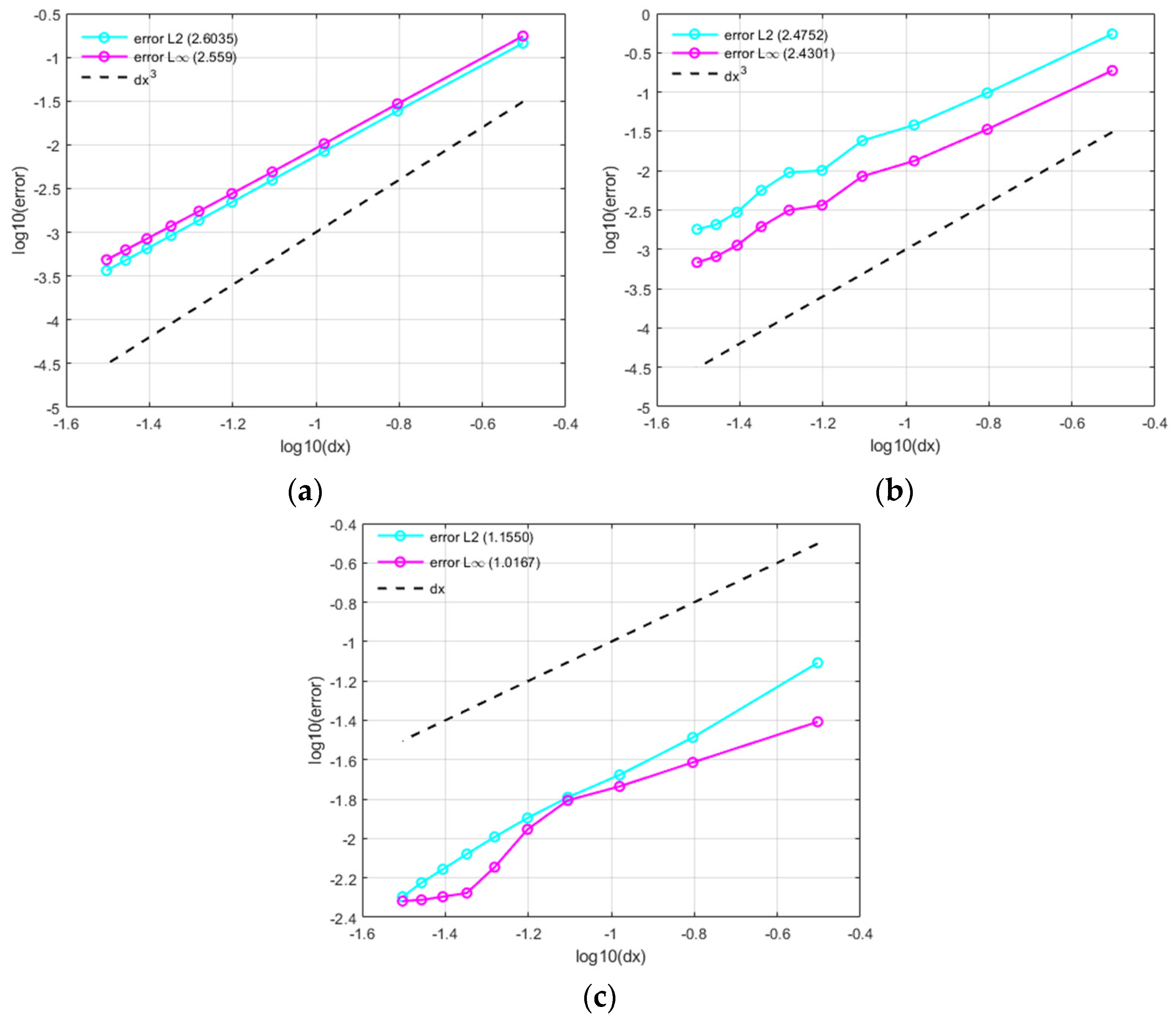
Figure 1. Illustration of the method for applying boundary conditions based on local regular-distributed particles: (a) Closure equations for background particles outside the boundary; (b) Closure equations for background particles inside the computational domain and closest to the boundary; (c) Closure equations for background particles closest to the fluid particles; (d) Integration region for boundary; (e) Integration region within the interior.
Jmse 11 02183 g001
Figure 2. Construction method of shape functions on 9−point cell, where the three different colors represent three different groups of construction units.
Jmse 11 02183 g002
Figure 3. Taylor–Green vortex field: solution of the pressure field in Ω = 0 , 2 π × 0 , 2 π at t = 10 4   s .
Jmse 11 02183 g003
Figure 4. Regular discretization of domain. The black dot, yellow dot, and blue dot, respectively, represent background particles, boundary particles, and fluid particles.
Jmse 11 02183 g004
Figure 5. Convergence of the pressure field for the Neumann boundary condition: (a) Least square-type interpolation; (b) MPS−LRBP (the combination of MPS method and LRBP method); (c) MPS−VPM (the combination of MPS method and VPM method).
Jmse 11 02183 g005
Figure 6. Irregular discretization of domain. The black dot, yellow dot, and blue dot, respectively, represent background particles, boundary particles, and fluid particles.
Jmse 11 02183 g006
Figure 7. 2-norm errors of coupled computation by background particles method.
Jmse 11 02183 g007
Figure 8. Pressure cloud map and error cloud map of a given particle distribution: (a) MPS−VPM; (b) MPS−LRBP.
Jmse 11 02183 g008
Figure 9. Particle distribution of triangle boundary (a) and circle boundary (b).
Jmse 11 02183 g009
Figure 10. Numerical and theoretical results of triangular boundary (above) and a quarter−circle boundary (below).
Jmse 11 02183 g010
Figure 11. Error cloud map of triangular boundary (above) and a quarter-circle boundary (below), where the left is MPS-VPM and the right is MPS-LRBP.
Jmse 11 02183 g011aJmse 11 02183 g011b
Table 1. Convergence study: grid parameters and order of convergence.
GridNxNyOrder of Convergence
LSMPS–LRBPMPS–VPM
E r r L 2 E r r L E r r L 2 E r r L E r r L 2 E r r L
1st2121
2.57142.57002.49222.48551.26050.6855
2nd4141
2.62012.58972.31562.27941.07740.6919
3rd6161
2.62502.57741.59351.56860.91370.5662
4th8181
2.61962.55993.90453.78511.08271.5220
5th101101
2.61062.54160.33370.80711.21382.4241
6th121121
2.60002.52383.39263.12121.29801.9567
7th141141
2.58892.50694.80214.07671.33340.3329
8th161161
2.57762.49103.06692.81461.34130.3075
9th181181
2.56652.47611.31291.63201.55380.1371
10th201201
Mean value2.59772.53742.57932.50781.23050.9582
Global value2.60352.55902.47522.43011.15501.0167
Disclaimer/Publisher’s Note: The statements, opinions and data contained in all publications are solely those of the individual author(s) and contributor(s) and not of MDPI and/or the editor(s). MDPI and/or the editor(s) disclaim responsibility for any injury to people or property resulting from any ideas, methods, instructions or products referred to in the content.

