

A Simple Bias Correction Scheme in Ocean Data Assimilation
Abstract
:1. Introduction
2. Model, Bias, Data and Bias Correction Scheme
2.1. Ocean Model
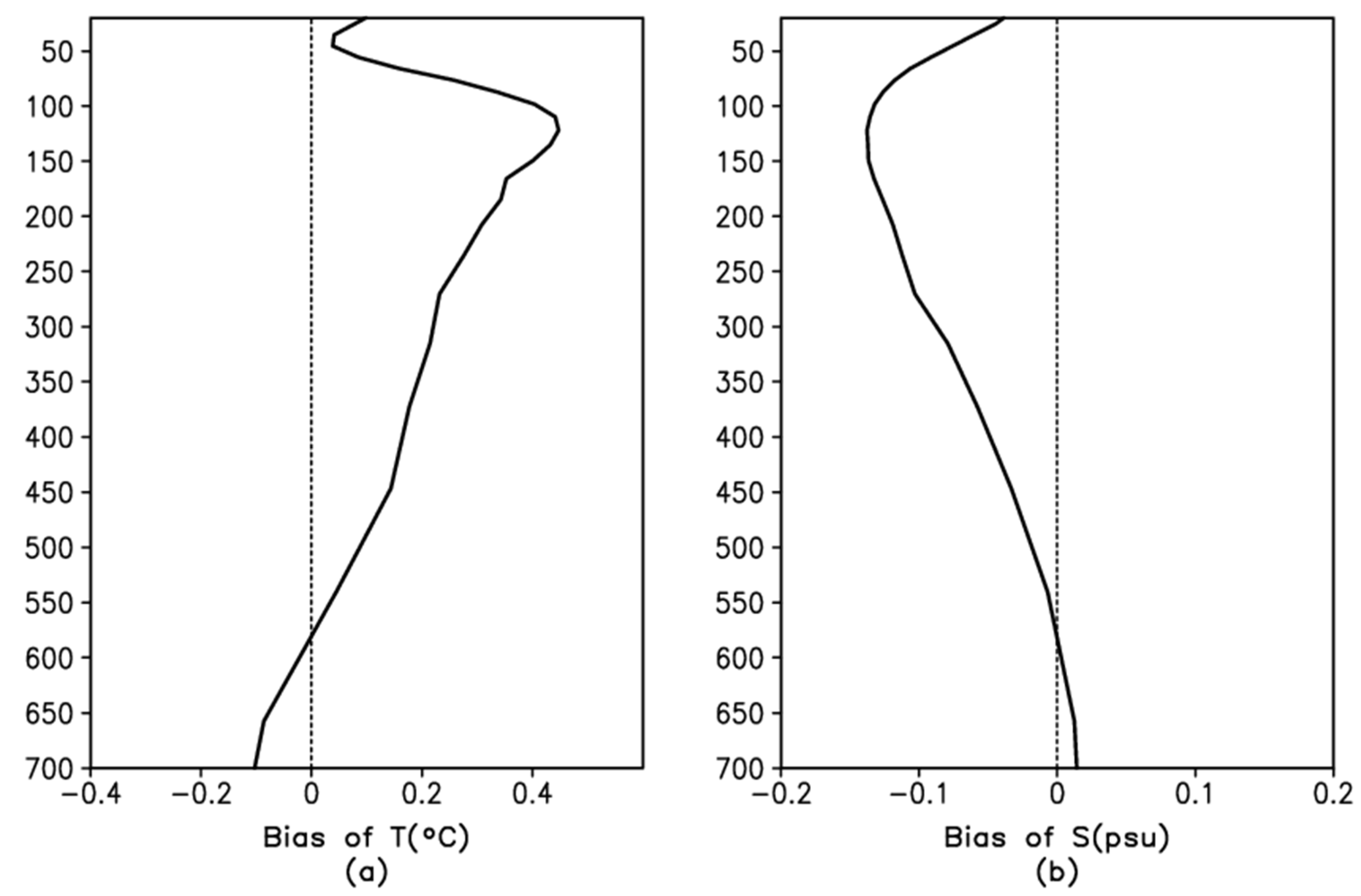
2.2. Model Bias
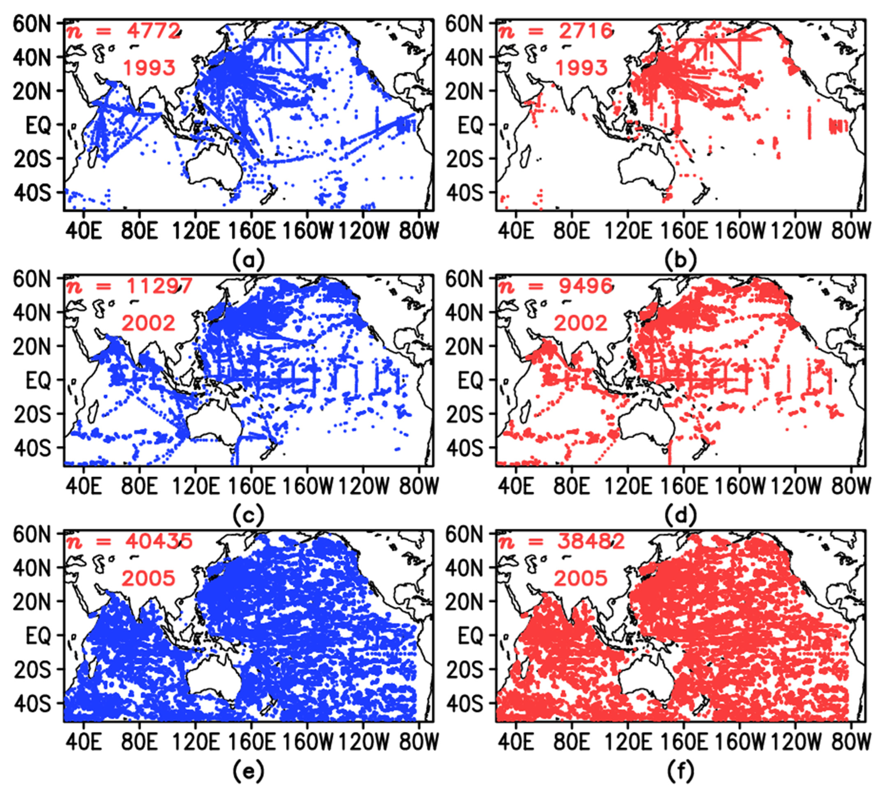
2.3. Data
2.4. The Bias Correction Scheme
3. Results
3.1. Experiment Setup
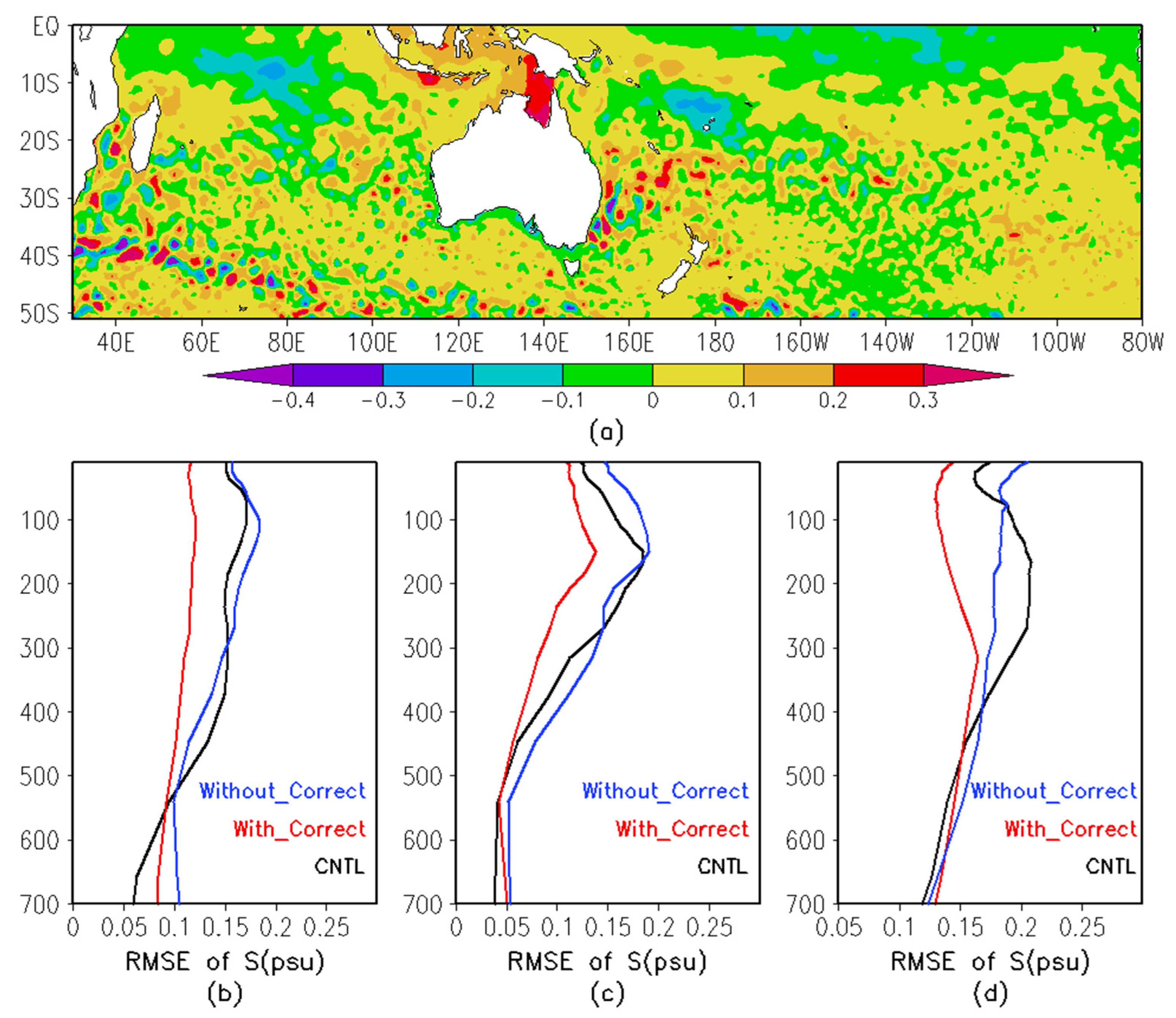
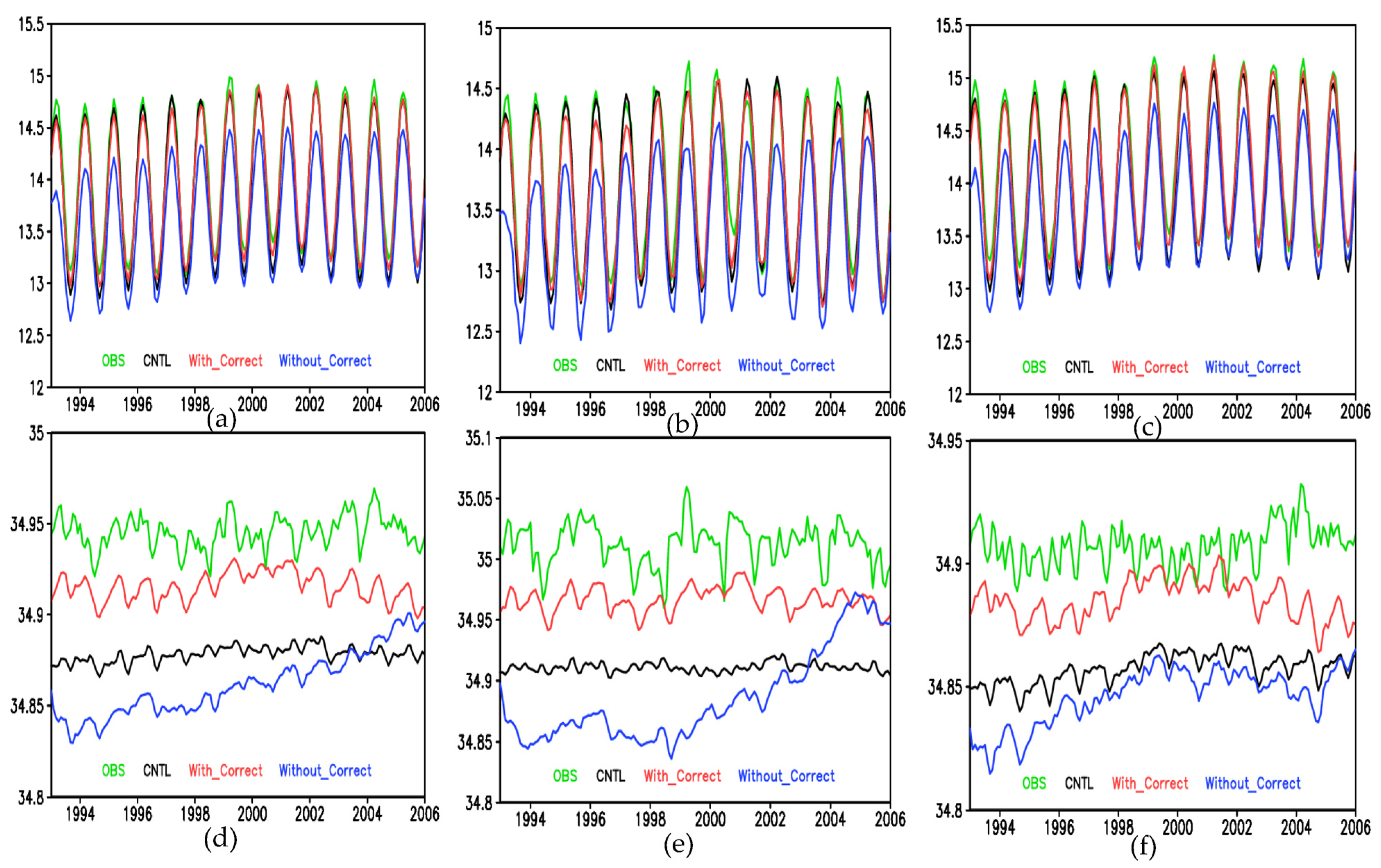
3.2. Impacts on Subsurface Temperature and Salinity
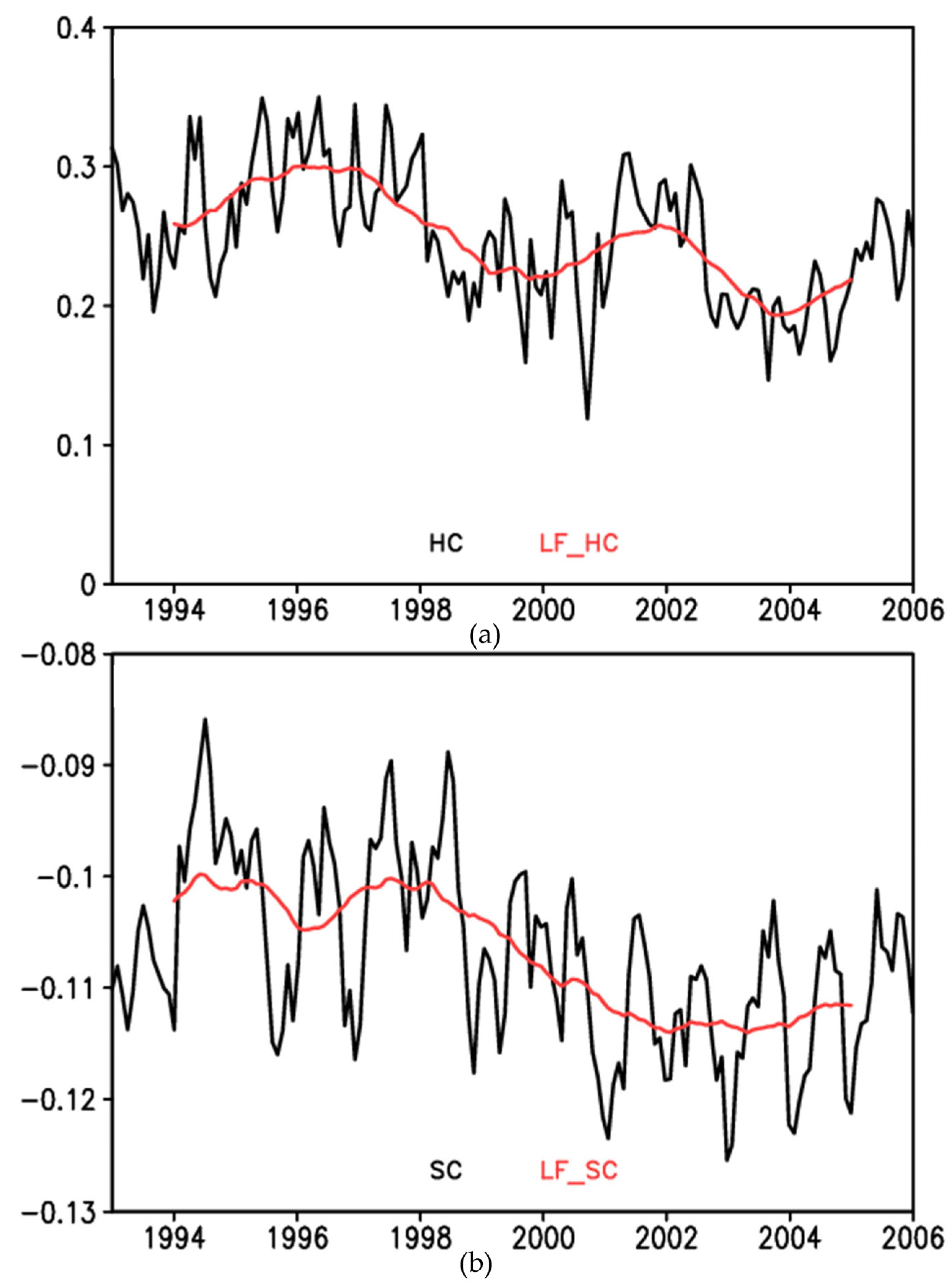
3.3. Impacts on the Heat and Salt Content
4. Discussion and Conclusions
Author Contributions
Funding
Institutional Review Board Statement
Informed Consent Statement
Data Availability Statement
Acknowledgments
Conflicts of Interest
References
- Artana, C.; Ferrari, R.; Bricaud, C.; Lellouche, J.M.; Garric, G.; Sennechael, N.; Lee, J.H.; Park, Y.H.; Provost, C. Twenty-five years of Mercator Ocean reanalysis GLORYS12 at Drake Passage: Velocity assessment and total volume transport. Adv. Space Res. 2021, 68, 447–466. [Google Scholar] [CrossRef]
- Han, G.; Fu, H.; Zhang, X.; Li, W.; Wu, X.; Wang, X.; Zhang, L. A global ocean reanalysis product in the China Ocean reanalysis (CORA) project. Adv. Atmos. Sci. 2013, 30, 1621–1631. [Google Scholar] [CrossRef]
- Pohlmann, H.; Jungclaus, J.; Marotzke, J.; Kohl, A.; Stammer, D. Improving predictability through the initialization of a coupled climate model with global oceanic reanalysis. J. Clim. 2009, 22, 3926–3938. [Google Scholar] [CrossRef]
- Balmaseda, M.A.; Alves, O.J.; Arribas, A.; Awaji, T.; Behringer, D.W.; Ferry, N.; Fujii, Y.; Lee, T.; Rienecker, M.; Rosati, T.; et al. Ocean initialization for seasonal forecasts. Oceanography 2009, 22, 154–159. [Google Scholar] [CrossRef]
- Hackert, E.C.; Kovach, R.M.; Busalacchi, A.J.; Ballabrera-Poy, J. Impact of Aquarius and SMAP satellite sea surface salinityobservations on coupled ElNiño/Southern Oscillation forecasts. J. Geophys. Res. Ocean. 2019, 124, 4546–4556. [Google Scholar] [CrossRef] [Green Version]
- Gao, C.; Zhang, R.; Wu, X.; Sun, J. Idealized experiments for optimizing model parameters using a 4D-Variational method in an intermediate coupled model of ENSO. Adv. Atmos. Sci. 2018, 35, 410–422. [Google Scholar] [CrossRef]
- Zheng, F.; Zhu, J. Roles of initial ocean surface and subsurface states on successfully predicting 2006–2007 El Niño with an intermediate coupled model. Ocean Sci. 2015, 11, 187–194. [Google Scholar] [CrossRef] [Green Version]
- Zhao, M.; Hendon, H.; Alves, O.; Yin, Y. Impact of improved assimilation of temperature and salinity for coupled model seasonal forecasts. Clim. Dyn. 2014, 42, 2565–2583. [Google Scholar] [CrossRef]
- Lellouche, J.M.; Greiner, E.; Le Galloudec, O.; Garric, G.; Regnier, C.; Drevillon, M.; Benkiran, M.; Testut, C.E.; Bourdalle-Badie, R.; Gasparin, F.; et al. Recent updates on the Copernicus Marine Service global ocean monitoring and forecasting real-time 1/12o high resolution system. Ocean Sci. 2018, 14, 1093–1126. [Google Scholar] [CrossRef] [Green Version]
- Eden, C.; Greatbatch, R.J.; Boning, C.W. Adiabatically correcting an eddy-permitting model using large-scale hydrographic data: Application to the Gulf Stream and the North Atlantic Current. J. Phys. Oceanogr. 2004, 34, 701–719. [Google Scholar] [CrossRef]
- Chepurin, G.A.; Carton, J.; Dee, D.P. Forecast model bias correction in ocean data assimilation. Mon. Wea. Rev. 2005, 133, 1328–1342. [Google Scholar] [CrossRef] [Green Version]
- Dee, D.P.; Uppala, S. Variational bias correction of satellite radiance data in the ERA-Interim reanalysis. Q. J. Roy. Meteorol. Soc. 2009, 135, 1830–1841. [Google Scholar] [CrossRef]
- Dee, D.P. Bias and data assimilation. Q. J. R. Meteorol. Soc. 2005, 131, 3323–3343. [Google Scholar] [CrossRef] [Green Version]
- Zuo, H.; Balmaseda, M.A.; Tietsche, S.; Mogensen, K.; Mayer, M. The ECMWF operational ensemble reanalysis–analysis system for ocean and sea ice: A description of the system and assessment. Ocean Sci. 2019, 15, 779–808. [Google Scholar] [CrossRef] [Green Version]
- Dee, D.P.; Da Silva, A.M. Data assimilation in the presence of forecast bias. Q. J. R. Meteorol. Soc. 1998, 124, 269–295. [Google Scholar] [CrossRef]
- Balmaseda, M.A.; Mogensen, K.; Weaver, A.T. Evaluation of the ECMWF ocean reanalysis system ORAS4. Q. J. R. Meteorol. Soc. 2013, 139, 1132–1161. [Google Scholar] [CrossRef]
- Dee, D.P.; Todling, R. Data assimilation in the presence of forecast bias: The GEOS moisture analysis. Mon. Wea. Rev. 2000, 128, 3268–3282. [Google Scholar] [CrossRef]
- Bell, M.J.; Martin, M.J.; Nichols, N.K. Assimilation of data into an ocean model with systematic errors near the equator. Q. J. R. Meteorol. Soc. 2004, 130, 873–893. [Google Scholar] [CrossRef]
- Balmaseda, M.A.; Dee, D.; Vidard, A.; Anderson, D.L.T. A multivariate treatment of bias for sequential data assimilation: Application to the tropical oceans. Q. J. R. Meteorol. Soc. 2007, 133, 167–179. [Google Scholar] [CrossRef] [Green Version]
- Fujii, Y.; Nakaegawa, T.; Matsumoto, S.; Yasuda, T.; Yamanaka, G.; Kamachi, M. Coupled climate simulation by constraining ocean fields in a coupled model with ocean data. J. Clim. 2009, 22, 5541–5557. [Google Scholar] [CrossRef]
- Shapiro, G.I.; Gonzalez-Ondina, J.M.; Salim, M.; Tu, J.; Asif, M. Crisis Ocean Modelling with a Relocatable Operational Forecasting System and Its Application to the Lakshadweep Sea (Indian Ocean). J. Mar. Sci. Eng. 2022, 10, 1579. [Google Scholar] [CrossRef]
- Bleck, R. An oceanic general circulation model framed in hybrid isopycnic-Cartesian coordinates. Ocean. Model. 2002, 4, 55–88. [Google Scholar] [CrossRef]
- Bertino, L.; Lisaeter, K.A.; Scient, S. The TOPAZ monitoring and prediction system for the Atlantic and Arctic Oceans. J. Oper. Oceanogr. 2008, 1, 15–18. [Google Scholar] [CrossRef] [Green Version]
- Sakov, P.; Counillon, F.; Bertino, L.; Lisaeter, K.A.; Oke, P.R.; Korablev, A. TOPAZ4: An ocean-sea ice data assimilation system for the North Atlantic and Arctic. Ocean Sci. 2012, 8, 633–656. [Google Scholar] [CrossRef] [Green Version]
- Large, W.G.; McWilliams, J.C.; Doney, S.C. Oceanic vertical mixing: A review and a model with a nonlocal boundary layer parameterization. Rev. Geophys. 1994, 32, 363–403. [Google Scholar] [CrossRef] [Green Version]
- Steele, M.; Morley, R.; Ermold, W. PHC: A global ocean hydrography with a high-quality Arctic Ocean. J. Clim. 2001, 14, 2079–2087. [Google Scholar] [CrossRef]
- Dee, D.P.; Uppala, S.M.; Simmons, A.J.; Berrisford, P.; Poli, P.; Kobayashi, S.; Andrae, U.; Balmaseda, M.A.; Balsamo, G.; Bauer, P.; et al. The ERA-Interim reanalysis: Configuration and performance of the data assimilation system. Q. J. Roy. Meteor. Soc. 2011, 137, 553–597. [Google Scholar] [CrossRef]
- Good, S.A.; Martin, M.J.; Rayner, N.A. EN4: Quality controlled ocean temperature and salinity profiles and monthly objective analyses with uncertainty estimates. J. Geophys. Res. Ocean 2013, 118, 6704–6716. [Google Scholar] [CrossRef]
- Cheng, L.; Zhu, J.; Cowley, R.; Boyer, T.; Wijffels, S. Time, Probe Type, and Temperature Variable Bias Corrections to Historical Expendable Bathythermograph Observations. J. Atmos. Ocean. Technol. 2014, 31, 1793–1825. [Google Scholar] [CrossRef]
- Gouretski, V.; Cheng, L. Correction for Systematic Errors in the Global Dataset of Temperature Profiles from Mechanical Bathythermographs. J. Atmos. Technol. Ocean. Res. 2020, 37, 841–855. [Google Scholar] [CrossRef]
- Zhang, R.H.; Wang, G.H.; Chen, D.; Busalacchi, A.J.; Hackert, E.C. Interannual biases induced by freshwater flux and coupled feedback in the tropical Pacific. Mon. Weather Rev. 2010, 138, 1715–1737. [Google Scholar] [CrossRef] [Green Version]
- Hackert, E.; Ballabrera Poy, J.; Busalacchi, A.J.; Zhang, R.H.; Murtugudde, R. Impact of sea surface salinity assimilation on coupled forecasts in the tropical Pacific. J. Geophys. Res. 2011, 116, C05009. [Google Scholar] [CrossRef] [Green Version]
- Pujol, M.I.; Faugere, Y.; Taburet, G.; Dupuy, S.; Pelloquin, C.; Ablain, M.; Picot, N. DUACS DT2014: The new multi-mission altimeter data set reprocessed over 20 years. Ocean Sci. 2016, 12, 1067–1090. [Google Scholar] [CrossRef] [Green Version]
- Reynolds, R.W.; Smith, T.M.; Liu, C.Y.; Chelton, D.B.; Casey, K.S.; Schlax, M.G. Daily high-resolution blended analyses for sea surface temperature. J. Clim. 2007, 20, 5473–5496. [Google Scholar] [CrossRef]
- Reynolds, R.W.; Banzon, V.F.; NOAA CDR Program. NOAA Optimum Interpolation 1/4 Degree Daily Sea Surface Temperature (OISST) Analysis, Version 2; NOAA National Centers for Environmental Information: Asheville, NC, USA, 2008. [Google Scholar]
- Argo. Argo Float Data and Metadata from Global Data Assembly Centre (Argo GDAC); SEANOE: La Spezia, Italy, 2000. [Google Scholar]
- Curry, R. HydroBase 2—A Database of Hydrographic Profiles and Tools for Climatological Analysis; Woods Hole Oceanographic Institution: Falmouth, MA, USA, 2001. [Google Scholar]
- Swift, J. Physical and Chemical Properties from Selected Expeditions in the Arctic Ocean; Digital Media; Dichtl, R., Axford, Y., Haran, T., Eds.; National Snow and Ice Data Center: Boulder, CO, USA, 2002. [Google Scholar]
- Sun, C.; Thresher, A.; Keeley, R.; Hall, N.; Hamilton, M.; Chinn, P.; Tran, A.; Goni, G.; Petit de la Villeon, L.; Carval, T.; et al. The data management system for the global temperature and salinity profile programme. In Proceedings of the OceanObs.09: Sustained Ocean Observations and Information for Society, Venice, Italy, 21–25 September 2009; Hall, J., Harrison, D.E., Stammer, D., Eds.; ESA Publication WPP-306: Paris, France, 2010; Volume 2. [Google Scholar] [CrossRef] [Green Version]
- Boyer, T.P.; Antonov, J.I.; Baranova, O.K.; Coleman, C.; Garcia, H.E.; Grodsky, A.; Johnson, D.R.; Locarnini, R.A.; Mishonov, A.V.; O’Brien, T.D.; et al. World Ocean Database 2013; Levitus, S., Mishonov, A., Eds.; NOAA Atlas NESDIS 72: Washington, DC, USA, 2013; p. 209. [Google Scholar]
- Guinehut, S.; Coatanoan, C.; Dhomps, A.-L.; Le Traon, P.-Y.; Larnicol, G. On the use of satellite altimeter data in Argo quality control. J. Atmos. Ocean. Technol. 2009, 26, 395–402. [Google Scholar] [CrossRef]
- Evensen, G. The Ensemble Kalman Filter: Theoretical formulation and practical implementation. Ocean. Dyn. 2003, 53, 343–367. [Google Scholar] [CrossRef]
- Gaspari, G.; Cohn, S.E. Construction of correlation functions in two and three dimensions. Q. J. Roy. Meteor. Soc. 1999, 125, 723–757. [Google Scholar] [CrossRef]
- Yan, C.; Zhu, J.; Tanajura, C.A.S. Impacts of mean dynamic topography on a regional ocean assimilation system. Ocean Sci. 2015, 11, 829–837. [Google Scholar] [CrossRef] [Green Version]
- Zhu, J.; Zheng, F.; Li, X. A new localization implementation scheme for ensemble data assimilation of non-local observations. Tellus A 2011, 63, 244–255. [Google Scholar] [CrossRef]
- Xie, J.; Zhu, J. Ensemble optimal interpolation schemes for assimilating Argo profiles into a hybrid coordinate ocean model. Ocean Model. 2010, 33, 283–298. [Google Scholar] [CrossRef]
- Lorenc, A.C.; Bell, R.S.; Macpherson, B. The Meteorological Office analysis correction data assimilation scheme. Q. J. R. Meteorol. Soc. 1991, 117, 59–89. [Google Scholar] [CrossRef]


| Experiment Name | Scheme | Assimilated Data | Assimilation Frequency | Period |
|---|---|---|---|---|
| Without_Correct | No bias correction | SST, SLA, T/S | 7 days | 1993–2005 |
| With_Correct | Bias correction | SST, SLA, T/S | 7 days | 1993–2005 |
| CNTL | No assimilation and no bias correction | None | N/A | 1993–2005 |
Disclaimer/Publisher’s Note: The statements, opinions and data contained in all publications are solely those of the individual author(s) and contributor(s) and not of MDPI and/or the editor(s). MDPI and/or the editor(s) disclaim responsibility for any injury to people or property resulting from any ideas, methods, instructions or products referred to in the content. |
© 2023 by the authors. Licensee MDPI, Basel, Switzerland. This article is an open access article distributed under the terms and conditions of the Creative Commons Attribution (CC BY) license (https://creativecommons.org/licenses/by/4.0/).
Share and Cite
Yan, C.; Zhu, J. A Simple Bias Correction Scheme in Ocean Data Assimilation. J. Mar. Sci. Eng. 2023, 11, 205. https://doi.org/10.3390/jmse11010205
Yan C, Zhu J. A Simple Bias Correction Scheme in Ocean Data Assimilation. Journal of Marine Science and Engineering. 2023; 11(1):205. https://doi.org/10.3390/jmse11010205
Chicago/Turabian StyleYan, Changxiang, and Jiang Zhu. 2023. "A Simple Bias Correction Scheme in Ocean Data Assimilation" Journal of Marine Science and Engineering 11, no. 1: 205. https://doi.org/10.3390/jmse11010205