1. Introduction
One of the important tasks of physical oceanography is an assessment of vertical turbulent exchange in the stratified waters of seas and oceans. In particular, the vertical flux of nutrients from the deep waters into the photic layer, where most biological production takes place, depends on the intensity of the turbulent exchange [
1,
2]. Knowledge of the vertical turbulent mass diffusion coefficient and the vertical gradients of nutrients (first of all, nitrates) would make it possible to quantify this flux in the sea and assess its significance for bioproductivity and the carbon cycle [
3].
The most reliable methods for estimating the coefficient of vertical turbulent mass diffusion are based on direct measurements of the turbulent energy dissipation rates and other parameters of hydrophysical microstructures on scales close to the Kolmogorov scale [
4]. Such studies involved special equipment, including free-falling or towing streamline apparatuses with microscale hydrophysical probes [
5,
6], and were carried out all over the world ocean [
7], including the Black Sea [
8,
9,
10]. As a result of these experimental studies, the profiles of turbulent energy dissipation rate ε(z), where z is depth, were determined and the coefficient of vertical turbulent diffusion K
ρ(z) was calculated using several methods, including the semi-empirical formula proposed by Osborn [
11]: K
ρ ≤ 0.2 ε/N
2, where N is the buoyancy frequency. However, direct measurements of turbulent exchange are rather difficult, and the vertical turbulent diffusion coefficient is often estimated on the basis of semi-empirical parameterizations and hydrophysical data with a much coarser resolution.
One such parameterization was proposed by Munk and Anderson [
12]. It was based on the dependence of the coefficient of vertical turbulent diffusion K
ρ on the Richardson number Ri in a stratified shear flow:
The exponent of the power function is often defined as n = 1.5, Ri = N
2/Sh
2, where N
2 = −g/ρ
0·∂ρ/∂z is the squared buoyancy frequency, Sh
2 = (∂u/∂z)
2 + (∂v/∂z)
2 is the squared vertical shear of the current velocity, and u and v are the eastern and northern velocity components, respectively. Following this pioneering paper, many authors [
13,
14,
15,
16,
17] applied modified formulas parameterizing the dependence of K
ρ on Ri. Basically, these formulas were defined as follows:
where K
0s, K
bs, α
s, and n
s are constants that depend on the vertical averaging scales of Ri. Here, K
0s represents mixing in the unstratified ocean, and K
bs is the background mixing by sources other than shear-induced instability.
Forryan et al. [
17] analyzed the parameterization (2) using the data of direct observations of vertical turbulent diffusivity from three separate ocean regions in the North Atlantic and Southern Ocean. It was found that equation (2) is robust for Ri > 1 at depths below the ocean near-surface boundary layer. In particular, when equation (2) was fitted to all the data for turbulent diffusivity from all three data sets simultaneously, then the best fit was for a smoothing window of 56 m with the following parameters: α
s = 1, n
s = 1.49, K
os = 3.62·10
−4 m
2/s, and K
bs = 8.14·10
−6 m
2/s.
For the Black Sea in particular, Stanev [
18] successfully used the parameterization proposed by Pacanowski and Philander [
13] for the numerical general circulation model of the Black Sea.
Zaron and Moum [
19] indicated that there are not enough dimensional groups in S
2, N
2, and K
ρ to provide a relation between K
ρ and Ri that is invariant to the dimensional units. In order to overcome this difficulty, they proposed a new parameterization, which is based not only on Ri but also included the shear length scale and the kinetic energy of the background flow. This parametrization appears to be very promisingand should be tried for the Black Sea.
Podymov et al. [
20,
21] estimated the values of K
ρ in the upper layer of the Black Sea (30–220 m) using the modified formula of Munk and Anderson and the Aqualog data of synchronously measured density and current velocity profiles from 2013 to 2016. It was shown that K
ρ varied from 10
−6 to 8.5·10
−3 m
2/s, and its average value was 8.8·10
–5 m
2/s, in agreement with the previous estimates of K
ρ for the same depth layer in the Black Sea [
22,
23] based on ship measurements using the LADCP current velocity profiles and data of the CTD casts. In the latter case, the dissipation rate of turbulent energy was calculated using the values of velocity shear and buoyancy frequency, smoothed with a 10 m vertical window. These values were close to the estimates of K
ρ obtained for the upper 20–80 m stratified layer in the Black Sea, based on direct measurements of the turbulent energy dissipation rate [
9].
Despite progress in the estimation methods for the coefficient of vertical turbulent diffusion in a shear flow of stratified fluids by using the parameterizations based on the Richardson number, there are at least two obstacles. First, the constant n in (1) can be less than 1.5 for small values of the Richardson number (Ri < 1) [
17]. Laboratory experiments with a mixing of stably stratified fluid resulted in a similar conclusion [
24]. Therefore, small values of the Richardson number could lead to uncertainty in the estimate. It is currently unclear which formula better suits such conditions. The second issue is that the Richardson number is a function of the vertical velocity shear and the buoyancy frequency, both of which depend on the averaging procedure, so the coefficient K
ρ should also depend on the size of the averaging window.
A possible approach to determine the vertical turbulent diffusion coefficient is based on the analysis of the fine structure (FS) of stratified ocean waters [
25]. Usually, an FS appears in vertical profiles of temperature, salinity, density, velocity, concentrations of passive and non-passive tracers, etc. It is characterized either by the presence of layers (whose thickness is up to several tens of meters) with low vertical gradients of these parameters, separated by high-gradient interlayers (step-like type), or by layers with temperature and salinity inversions compensated in density (intrusive type). For the latter, a change in the sign of the vertical gradient to the opposite, in comparison with the sign of the background gradient, is considered an inversion.
An FS can have a reversible or irreversible nature. The reversible FS is usually associated with internal waves and their kinematic effect, which leads to adiabatic deformations in temperature and salinity profiles. The irreversible FS occurs as a result of internal vertical mixing events or quasi-isopycnic intrusions, both causing non-adiabatic profile changes and producing vertical and lateral fluxes in mass and momentum. In contrast to fluctuations of an isotropic turbulent nature, ocean FS layers have horizontal extensions usually 10
2–10
4 times larger than their vertical thickness [
25].
FSs in different parts of the world ocean were the subject of many detailed studies during the last 40–50 years. Much attention was paid to transfrontal thermohaline intrusions, whose dynamics largely depend on buoyancy fluxes caused by differential diffusion–convection. Among the publications on this subject, we would like to mention the pioneering work of Joyce [
26] and a review by Ruddick [
27], which focused on the theory of intrusions and their laboratory modeling. In the case of Black Sea regional oceanography, investigations were mostly concerned with the intrusive type of FS formed via the intrusions of modified waters of the lower Bosphorus current into the Black Sea pycno-halocline and deeper layers [
28,
29]. Reliable evidence for such intrusions was found recently, based on the analysis of the vertical profiles of temperature, salinity, and dissolved oxygen obtained with the Argo floats [
30,
31,
32,
33].
A new step in the study of the Black Sea intrusions was conducted by Stanev et al. [
34]. It was shown that optical backscattering coefficient data from the bio-Argo floats with a vertical resolution of 1 m can be successfully used to indicate thermohaline intrusions in the Bosphorus region and to the east of it. In this area, this coefficient is more than five times larger than elsewhere and could be an indicator of bacterial abundance and biological involvement in the precipitation of manganese-containing particles. The observations clearly identify thermal and «particle» intrusions down to ~700–800 m in the Bosphorus inflow area.
More recently, isopycnic mesoscale (20–50 km) thermohaline anomalies were identified and analyzed in the upper 300 m layer of the Northeastern Black Sea based on the archive of the ship-born CTD-data along 100 nautical miles cross-sections between the coastal zone and the deep part of the sea [
35]. It was shown that the FS in the temperature profiles was mostly of the intrusive type at the boundaries of the thermohaline anomalies where an absolute value of the product ΔT [(φ
ro − φ
T)
2]
1/2 was sufficiently large. Here, ΔT is the value of the isopycnic temperature anomaly between two CTD-stations, and φ
ro – φ
T is the angle between isotherms and isopycnals. The observed temperature inversions did not result in density inversions. Their formation was due to quasi-isopycnic intrusions at the thermohaline fronts at the boundaries of the mesoscale thermohaline anomalies. Yet the number of profiles with the FS temperature inversions at each cross-section was much less than the number of profiles with the step-like FS associated with multimode internal waves and vertical turbulent mixing processes. It should be noted that the conditions for double-diffusive convection are lacking in the upper 300 m of the Black Sea [
36]. Therefore, it could not be attributed any role in the formation of the step-like FS.
Part of the step-like FS is formed due to vertical mixing processes caused by breaking internal waves and shear flow instability. The latter mechanism seems to prevail in the Black Sea Rim Current zone (see below), where significant vertical velocity shear is observed from time to time. In such cases, the Richardson number has low values and the intensity of vertical turbulent mixing increases [
9,
37]. As it was shown in [
9], a decrease in the bulk Richardson number, estimated using geostrophic velocity shear and CTD measurements of density vertical distribution, was associated with the FS interleaving intensity (a magnitude of deviation in the smoothed temperature, salinity, and density profiles from the original measurements) in the seasonal thermocline and the permanent pycno-halocline. At the same time, the FS intensity increases along with the turbulent energy dissipation, as was revealed in experiments with the free-falling microstructure probe Baklan [
5]. However, these preliminary results require further research based on more numerous observations.
Of course, there is difficulty in extracting a turbulent mixing signal from FS data, since non-breaking internal waves and intrusion processes cause deformation in the density profile [
25]. Furthermore, a standard CTD sampling is usually performed using a probe lowered from a ship on a conducting wire cable. This results in data pulsations, caused by cable jerking and probe snaking because of ship pitching, thus producing an artificial fine-scale vertical distribution of the thermohaline parameters. A particularly strong noisiness in fine-structure data should be expected when using massive rosette (carousel) complexes with water sampling bottles. This kind of measurement is conventionally used in multidisciplinary ocean studies. To reduce the data noise as much as possible, a free-falling CTD probe with a streamlined shape should be used [
38,
39]. However, such measurement methods are far from being widespread.
This paper presents the results of the studies of the FS characteristics of density profiles in the Northeastern Black Sea and their dependence on the Richardson number, based on the large dataset composed of synchronized and accurate measurements of density and current velocity profiles using the moored profiler Aqualog [
40]. The Aqualog was deployed at the upper part of the continental slope within the zone of the Rim Current, which is a basin-scale current that encircles the Black Sea in a counterclockwise direction [
28]. The main reason for the formation of a cyclonic annular current in the Black Sea is the cyclonic vorticity of the wind stress on its surface [
18,
41,
42]. As was shown with a drifter experiment, the typical speed of the Rim Current in the upper layer is about 0.15–0.2 m/s, and it can increase up to 0.8–0.9 m/s [
43,
44]. Due to the sharp pycno-halocline located at a depth of 100–200 m, the current velocity decreases rapidly with depth in the upper 250 m layer, resulting in substantial velocity shear [
45].
The Rim Current core is usually observed further into the deep sea than the Aqualog location. However, due to meandering, from time to time, the current moves close to the shore, and the Aqualog registers a significant increase in the flow velocity directed to the northwest. This happens when the mooring station moves into a cyclonic meander of the Rim Current. When it moves into an anticyclonic meander (or a mesoscale anticyclonic eddy), a southeastern countercurrent is observed. A typical period of a change in the velocity direction in the study area is about 10 days [
46].
The aim of this work was to find the interrelations between the Black Sea FS characteristics of density profiles and the vertical turbulent exchange based on the Aqualog measurements. The data and methods are described in
Section 2. The evidence for the dependence of the FS characteristics of the density profiles on the Richardson number is demonstrated in
Section 3.1 and their interrelation with vertical turbulent exchange is analyzed in
Section 3.2, along with their application for estimating the coefficient of vertical turbulent mass diffusion. The discussion of the results is contained in
Section 4 and the preliminary conclusions in
Section 5.
2. Materials and Methods
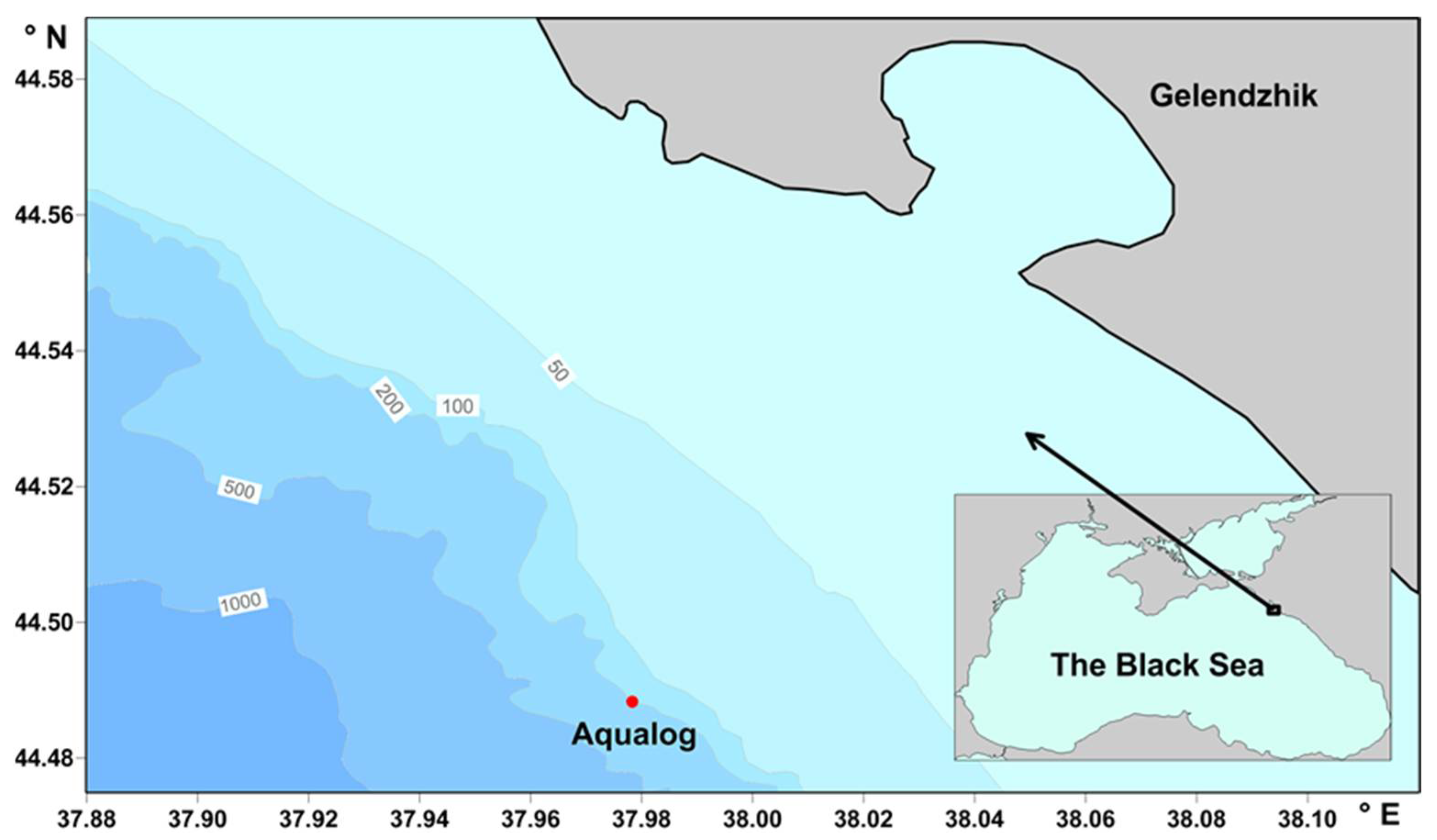
The analyzed data were collected using the autonomous moored profiler Aqualog [
40] located on the continental slope, five nautical miles from the Black Sea coast near the town of Gelendzhik (
Figure 1). The mooring depth was about 240 m.
The Aqualog profiler is capable of moving up and down along the mooring line stretched between the bottom anchor and the top floatation. The latter was positioned about 30 m below the sea surface—deep enough to avoid any significant effect on it from the surface waves (
Figure 2).
Because of the stable propulsive force and streamlined body of the device, its speed along the mooring cable was stable (about 20 cm/s on average, with an SD of about 0.7 cm/s), varying within a few cm/s (
Figure 3). During the observational survey, the Aqualog was equipped with the CTD probe Idronaut Ocean Seven 316 to measure temperature and salinity with a vertical resolution of 8–10 cm and the Doppler acoustic current meter Nortek Aquadopp 3D to measure current velocity with a vertical resolution of about 1 meter. Hence, the Aqualog was a reliable tool for the accurate measuring of the hydrophysical parameters with a fine vertical resolution.
Below, we analyze the data obtained with the Aqualog from 25 October 2015 to 1 March 2016. The profiler operated continuously for 129 days, measuring the vertical profiles of the hydrophysical parameters every 6 h from the subsurface floatation downward to a depth of about 220 m. All measured parameters, including the current velocity, were binned into 1 m vertical cells and considered as primary data.
While the Doppler acoustic current meter Aquadopp provided us with high quality data, there was still a measurement error that could lead to extremely high values of Ri when velocity was rather low and density gradient was high, causing distortions in the Ri-based estimations. To remove these errors, the following procedure was used to calculate the vertically averaged Richardson number. The profiles of N
2(z) and Sh
2(z) were smoothed with a vertical moving average window of 25 m. The width of the window was chosen to overlay the FS layers, of which thickness usually did not exceed 10 m [
9]. Henceforth, we shall use the angle brackets (<...>) to indicate that a certain parameter was smoothed in a 25 m averaging window, or its calculation was based on similarly smoothed components. The values of <N
2> and <Sh
2> were used to obtain the average Richardson number <Ri> = <N
2>/<Sh
2> that characterized the stratified shear flow stability, the intensity of the vertical turbulent exchange, and the FS characteristics.
One of the most important methodological aspects of this work was the procedure of FS extraction from the primary data profiles. Let us note that the FS variability of the potential density profiles σ(z) was determined with the variability of the density gradient Δσ/Δz, which characterized the density stratification of the aquatic environment. The density gradient was calculated from the primary vertical distribution of density as Δσ/Δz, where Δσ is the density difference between the lower and upper points of the density profile with a distance of Δz = 1 m between them. The gradient magnitude may vary widely, and the gradient changes its sign in the layers in which the stable stratification is locally overturned. The FS variations appear around the averaged values of Δσ/Δz. To calculate the average gradient <Δσ/Δz> we used the same moving average procedure with a 25 m window as that for the calculation of <Ri>. The fluctuating part (pulsation) of the density gradient was defined as the difference between the primary and the averaged gradient: (Δσ/Δz)′ = Δσ/Δz − <Δσ/Δz>.
Typical profiles of the density gradient and its pulsations are presented in
Figure 4. Let us consider an element of FS as a layer situated between consecutive odd crossings of the original profile with the smoothed profile (transition through zero for (Δσ/Δz)′). Such an element with the thickness h contains both positive and negative anomalies of Δσ/Δz and could appear after an incomplete vertical mixing. The negative anomaly can be associated with a partly mixed portion of the profile and the positive anomaly, with the interface between the negative anomalies.
Along with the calculations of the thickness of all h-elements for all acquired profiles, we also calculated the thickness of the layers with positive and negative gradient anomalies (sublayers of h element, denoted as h+ and h−, respectively), as well as the thickness of the density gradient inversion layers, hinv.
The following procedure was used to estimate the thickness of the density gradient inversion layers. Since these layers were relatively thin (their thickness in most cases was less than 1 m), the original CTD data were binned into 10 cm vertical cells and smoothed with a 1 m moving average. Since the density of water in the Black Sea generally increases with depth, the inversion layers were those where the density decreased with depth. All acquired profiles were scanned from top to bottom. The thickness hinv of every inversion layer was calculated as an absolute depth difference between the bin, where density decreased with depth compared with the overlying (upper) bin, and the first underlying (lower) bin, where density increased with depth again. Therefore, the estimation error was ±10 cm. To cut off insignificant density fluctuations inside the step-like FS and minor probing errors, the density fluctuations smaller than 0.001 kg/m3 were ignored.
Since the Richardson number was calculated with a 1 m vertical step, to find a connection between <Ri> and the hinv intervals, the values of <Ri> were interpolated over a uniform 10 cm vertical grid, matching the 10 cm CTD data cells used for the hinv calculation. After that, <Ri> was calculated for every hinv, as a mean value of <Ri> over all the 10 cm cells that fell within a particulate hinv layer.
To estimate the non-dimensional intensity of the FS density gradient pulsations we used a form of the Cox number [
47]. Initially [
48,
49], this number was introduced as a dimensionless quadratic measure of microstructural fluctuations in temperature and salinity. In our case, the “fine scale” analog of this number has the following expression:
To calculate <C(z)>, the profile of the squared values of density gradient pulsations (Δσ/Δz)′
2 was smoothed with the same 25 m window, as indicated by the angle brackets in (3). The values of <C(z)> and their dependence on <Ri> will be used to find the relationship between <C(z)> and the turbulent mass diffusion coefficient K
ρ (see
Section 3.2 below).
To calculate the turbulent mass diffusion coefficient K
ρ with Equation (2), we used the same “Aqualog” data, a 40 m smoothing window, and the previously obtained coefficients [
20]: α
s = 0.2, n
s = 1.5, K
0s = 10
–3, and K
bs = 10
−6.
4. Discussion
As was mentioned in the introduction, an estimation of the coefficient of vertical turbulent mass diffusion in a stratified water column is an important oceanographic problem. Ri-based parameterization of this coefficient is not always applicable since it involves both CTD data and data on the vertical distribution of the flow velocity or its vertical shear. Such data are present if the profiles of temperature, salinity, and current velocity are measured simultaneously with a CTD probe and either a ship-mounted ADCP or an LADCP in the profiling mode [
22]. However, CTD data are usually not supplemented with the current velocity profiles. There is a lot of information on the vertical distributions of sea temperature, salinity, and density with the FS resolution missing the quasi-synchronous data on the current velocity shear. The question is whether the data of the CTD measurements alone could be successfully used to estimate the coefficient of vertical turbulent diffusion or not. We tried to address this challenge by analyzing the measurement data obtained using the moored profiler Aqualog in the Black Sea.
The estimates of the averaged Richardson number <Ri> based on the Ri values obtained for the high-resolution (one meter) data seem to be quite realistic. The smoothing of the N
2 and Sh
2 profiles with a 25 m moving average, before using them for the Ri calculation, made it possible to denoise the estimates and obtain a <Ri> that is a reliable characteristic of the stratified shear flow stability. It may serve as a criterion for the dynamical status of the flow. When the velocity shear is strong enough, the <Ri> values comply with the criterion of Miles–Howard for shear instability. Another piece of evidence in support of the reliability of this estimation is that almost all density inversions during the observed events of vertical mixing (overturning of stratified water layers) occur when <Ri> < 0.25 [
50]. However, we should use the calculations of density inversions with caution, since they are usually performed at the lower limit of the sensors’ vertical resolution and may be affected by measurement errors.
An important role in finding the correlation between the values of the FS Cox and Richardson numbers was the additional ensemble averaging of these parameters with a 5-day (20 profiles) moving average along the density surfaces. As it was shown earlier, a typical period of mesoscale variability is about 10 days in the zone of the Rim Current [
46,
55]. Therefore, a 5-day average retains the mesoscale variability caused by meandering and eddy formation in the Rim Current area.
Another important factor is that the energy of internal waves in the Black Sea is relatively small compared with the ocean since the Black Sea belongs to non-tidal seas and is characterized by moderate wind forcing [
22,
23]. Thus, the processes of vertical mixing and FS formation depend mostly on the velocity shear produced by the highly baroclinic Rim Current and mesoscale eddies [
9]. It should be noted that the strong dependence of the vertical mixing on the current velocity shear is characteristic not only of the Rim Current but also of other jet-like currents, for example, the western boundary currents [
15].
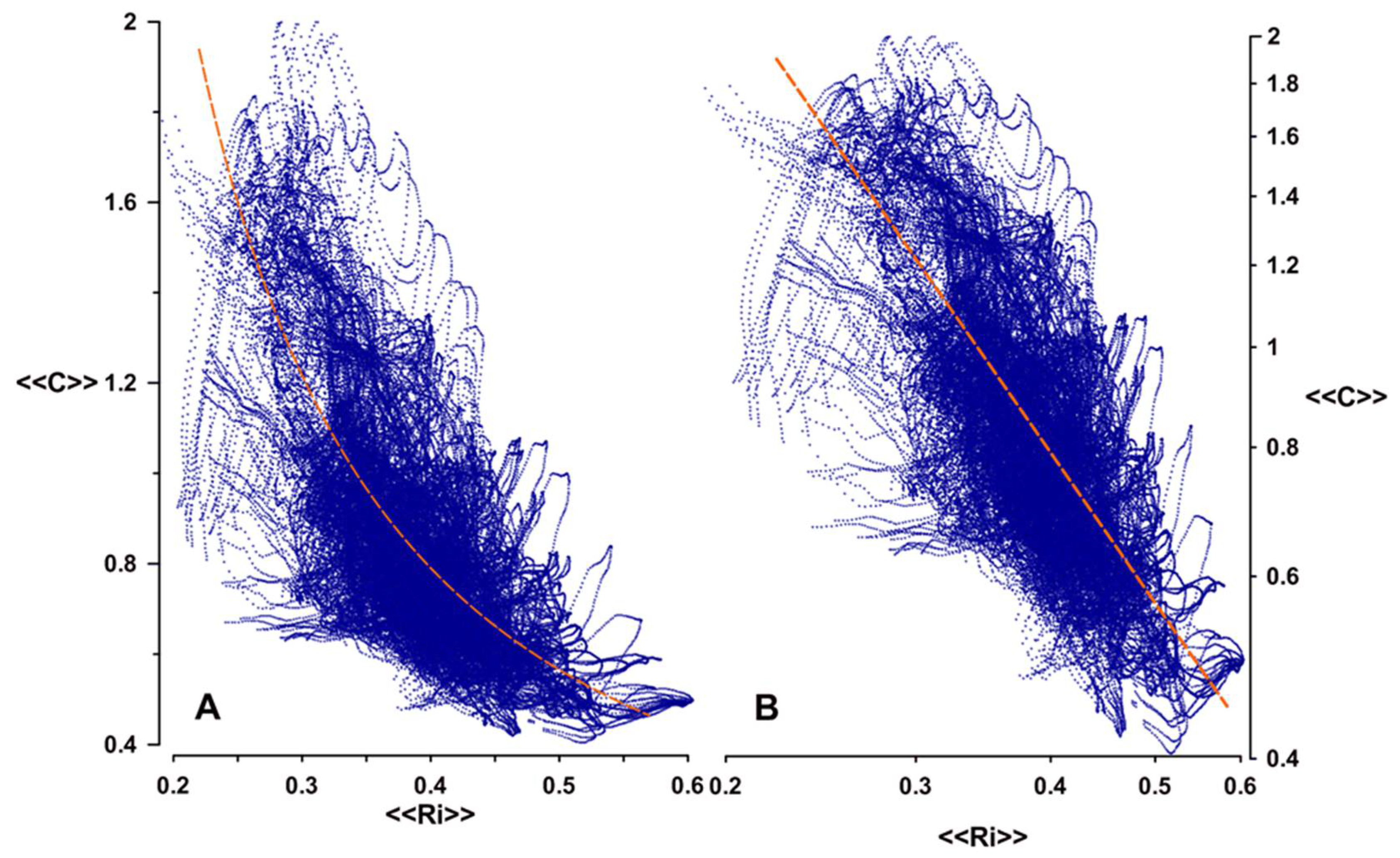
The ensemble averaging of <C> and <Ri> provided us with an opportunity to look for a correlation between these parameters. It was found that <<C>>~(<<Ri>>)
−n when n = 1.5 with a Pearson correlation coefficient R = 0.68 (RMSE = 0.35). Since the same power function with the same exponent n was successfully used by Podymov et al. [
20,
21] for the parameterization of the coefficient of vertical turbulent mass diffusion K
ρ, it was plausible to assume that a linear correlation exists between <<C>> and <<K
ρ>>, where <<K
ρ>> was calculated using the same Aqualog data and averaged in the same manner as <<C>>. We obtained a statistically significant linear correlation, although with a smaller correlation coefficient (R = 0.54).
The relationship found between the FS Cox number and the coefficient of vertical turbulent mass diffusion is only one step in a study of the FS characteristics and their dependence on the intensity of the vertical turbulent exchange in the Black Sea. In the future, it would be plausible to apply Thorpe’s and Ellison’s scales to the Aqualog data in order to estimate the turbulent energy dissipation velocity, as it was performed in, e.g., [
56], and use it to calculate the turbulent mass diffusivity. The advanced methods for K
ρ calculation proposed by Zaron and Moum [
19], or Gregg et al. [
57] (as formalized by Kunze et al. [
58]), also appear worth trying (e.g., [
59]), using the high-resolution and long-term data obtained with the Aqualog profilograph.
5. Conclusions
We analyzed the data of continuous long-term measurements of the vertical distribution of density and current velocity in a depth range of 30–220 m sampled using the autonomous Aqualog profiler moored at the upper part of the Black Sea continental slope. The fine structure of the vertical density gradient and its relation to the averaged values of the Richardson number <Ri> was estimated using high-resolution (one meter) data on the vertical distributions of water density and current velocity.
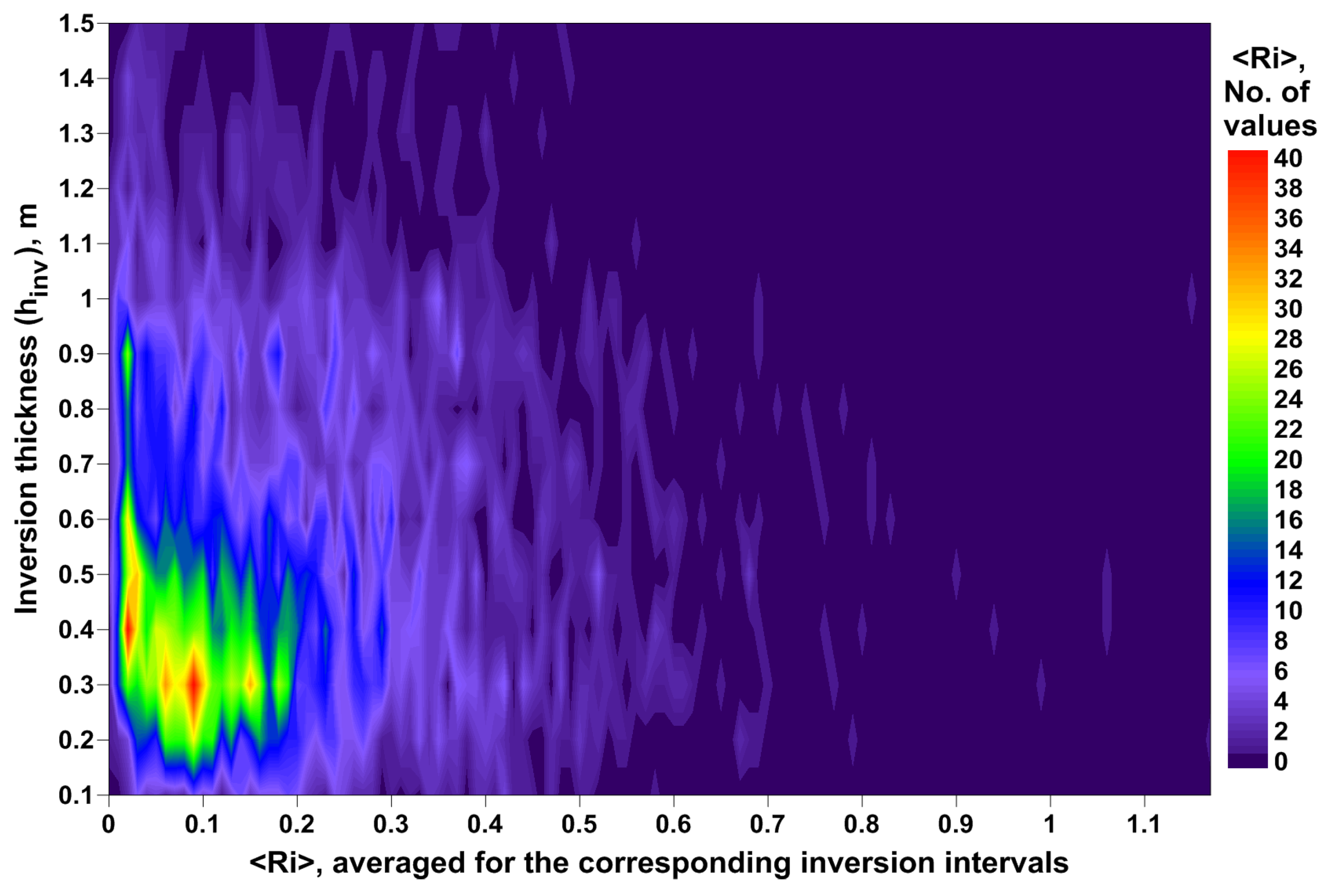
Two important fine-structure characteristics were calculated: the thickness of layers with increased and decreased density gradients and the thickness of layers with inversions of the density gradient. Based on the density gradient profiles binned into 1 m vertical cells, it was revealed that the thickness of a typical vertical fine-structure element (a layer of increased density gradient and an underlying layer of decreased density gradient) is about 10 times larger than the mean thickness of layers with density inversions calculated over a 10 cm vertical grid.
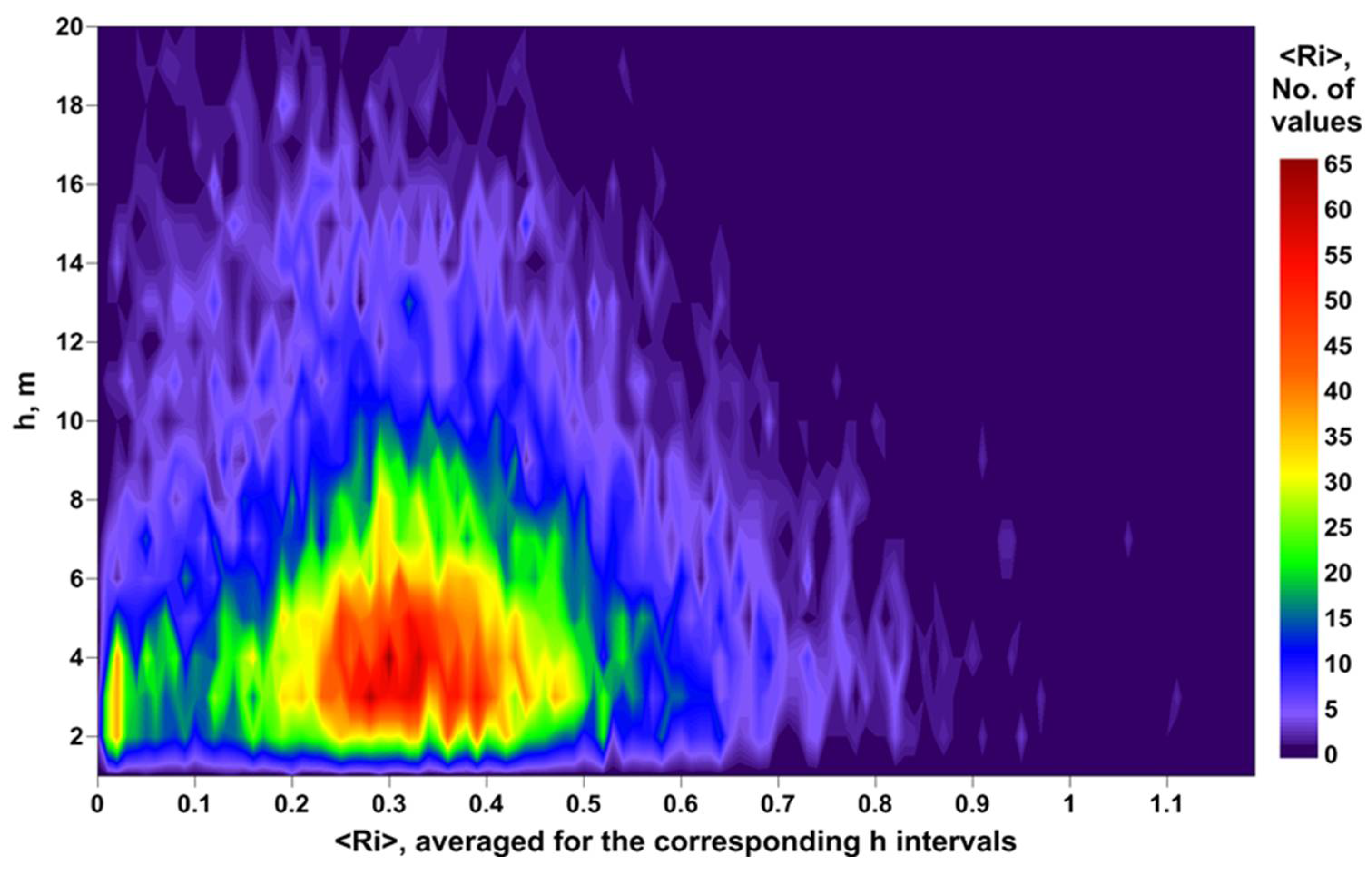
Most fine-structure elements corresponded to the values of <Ri> from 0.2 to 0.5, while the density inversions were mostly observed when <Ri> < 0.25. Their amount was significantly less than the number of fine-structure elements. The existence of density inversions is fundamentally important because they indicate the ongoing process of vertical turbulent mixing, i.e., the overturning of stably stratified water layers, leading to the formation of irreversible elements in the fine structure. It also proves that the parameters of the fine structure are related to the processes of vertical turbulent mixing, which strongly depend on the Richardson number.
The Cox number C for the fine structure was calculated, and it was found that after vertical and temporal averaging, <<C>> correlated with the Richardson number <<Ri>> averaged in the same manner. Particularly, it was shown that <<C>>~(<<Ri>>)
−1.5 with Pearson correlation coefficient R = 0.68 and root-mean-square error RMSE = 0.35. The coefficient of vertical turbulent mass diffusion K
ρ had a similar power dependence on Ri, as was estimated earlier [
20,
21] for the Black Sea cold intermediate layer and pycno-halocline. Based on this result we found a linear correlation between <<C>> and <<K
ρ>>, with Pearson correlation coefficient R = 0.54 and RMSE = 5·10
−5 between Ri-based <<K
ρ>> values and a <<C>>-based approximation. This is about 1.5 times less than the median value of the turbulent vertical mass exchange coefficient itself.
The results of this work suggest that in the future, it might be possible to provide Kρ estimations for the Rim Current zone of the Black Sea using the fine-structure characteristics of density profiles without any calculations of the Richardson number. It means that only the data of high-quality CTD measurements performed under certain hydrodynamic and meteorological conditions would be required for this procedure, and the estimation of Kρ would be significantly facilitated. However, more work is required to refine the methods for a quality estimate of the vertical turbulent diffusion coefficient and to determine which of the fine-structure elements of density (temperature and salinity) profiles are best suited to reflect the processes of vertical mixing in a stratified fluid.


