Predictive Modeling of Eastern Little Tuna (Euthynnus affinis) Catches in the Makassar Strait Using the Generalized Additive Model

Abstract

The Makassar Strait (MS) is characterized by water mass from the Pacific Ocean and is one of the ITF (Indonesia Throughflow) branches. It carries warm water masses from the Pacific Ocean to the Indian Ocean. This research aims to analyze the relationship between CPUE of Eastern Little Tuna (Euthynnus affinis) and oceanographic variables, likewise predict the fishing area using the Generalized Additive Model (GAM). The research method used is spatial and temporal analysis. The data was used from 2015 to 2020. The data processed were sea surface temperature, chlorophyll-a, salinity, currents, sea level as predictor variables, and Eastern Little Tuna production as a response. Eastern Little Tuna catch data were normalized into Catch per Unit Effort, while the oceanographic data were extracted using ArcGIS. Based on the results of the GAM model, it was found that the model with five variables is the most suitable predictive model, with 16.4% CDE. Salinity is the most influential parameter on the catch of Eastern Little Tuna with a significance value of <2.00 × 10⁻¹⁶ ***. The optimum value for SST is 30–31 °C, chlorophyll-a is 1–2 mg/m³, salinity is 29–30 ppt, current velocity is 0.3–0.5 m/s and sea level is between 0.6–0.7 m. Based on the GAM prediction results, a high CPUE value will be obtained in the southwest monsoon (March to May). Fishing activity carried out in the best season will implement the adoption of harvest control measures.

1. Introduction

Indonesia has Fisheries Management Area (FMA) that is intended for controlling the fisheries management activities [1], which include supporting fish resource management policies [2]. The Makassar Strait (MS) is part of FMA 713, contributing to Indonesia’s second-largest fish production [3]. The Indonesian Statistical Data Agency stated that in 2019, 558,000 tons of fisheries production were obtained from FMA-RI 713.

The MS is connected to the Pacific Ocean (PO) in the north, the Java Sea, and the Flores Sea in the south [4]. MS is also known as one of the branches of ocean thermohaline circulation, which carries warm water masses from the PO to the Indian Ocean (IO). These conditions make the water mass stratification in MS identifiable [5]. Warm water masses from the PO to the IO will affect the temperature in the MS [6]. The productivity of the MS waters occurs throughout the year, both in the west and east monsoonal seasons [7]. The MS has the potential for fish resources, especially groups of pelagic fish [8,9].

One of the major commodities in the MS waters is Eastern Little Tuna, which has become the main export commodity [3]. The Indonesian statistical data agency reported that for the 2020 period, this category produced around 91,405,337 kg. Based on data from the Directorate General of Capture Fisheries (DGCF), Eastern Little Tuna (Euthynnus affinis) is included in the Fishery Management Plan (RPP). However, the status of the utilization level of Eastern Little Tuna in FMA 713 for 2020 is unknown (Ministry of Maritime Affairs and Fisheries of the Republic of Indonesia, 2020). To regulate the number of catches per monsoon, it is necessary to optimize catches based on temporal and spatial data.

The mapping of the Eastern Little Tuna fishing area was carried out using Generalized Additive Model (GAM). The GAM was used to determine the most suitable Eastern Little Tuna habitat by selecting the best predictor variables. It consists of a collection of non-parametric and semi-parametric regression techniques to explore the relationship between response variables and predictors [10]. Several parameters affect fish distribution, including sea surface temperature and chlorophyll-a [11], salinity [12], and ocean currents [13]. Studies using GAM have been carried out on various migratory species distribution and catch prediction, such as Eastern Little Tuna in west Java, where it was found that chlorophyll-a was the most influential parameter on CPUE [14], albacore tuna [15], catfish and squid [10], yellowfin tuna [16,17]. Syamsuddin et al. (2013) used GAM to determine the effect of El Nino-Southern Oscillation events on catches of Bigeye Tuna [18]. Swathi et al. (2019) used GAM to assess fish abundance spatial occupancy in the northeast Bay of Bengal [19].

In principle, the estimation of fishing grounds is to look for the relationship between oceanographic parameters and schools of fish. The predictor approach is used to determine the relationship between fish resources and environmental factors that are not linear [20]. This study aims to analyze the relationship between the CPUE of Eastern Little Tuna (Euthynnus affinis) and oceanographic variables to develop preferences for Eastern Little Tuna habitat models using the GAM. The purpose of this study was to analyze the relationship between oceanographic parameters and the catches of the Eastern Little Tuna in the Makassar Strait. This study also aims to predict the CPUE of Eastern Little Tuna based on its habitat through the statistical approach Generalized Additive Model (GAM) in the Makassar Strait.

2. Materials and Methods

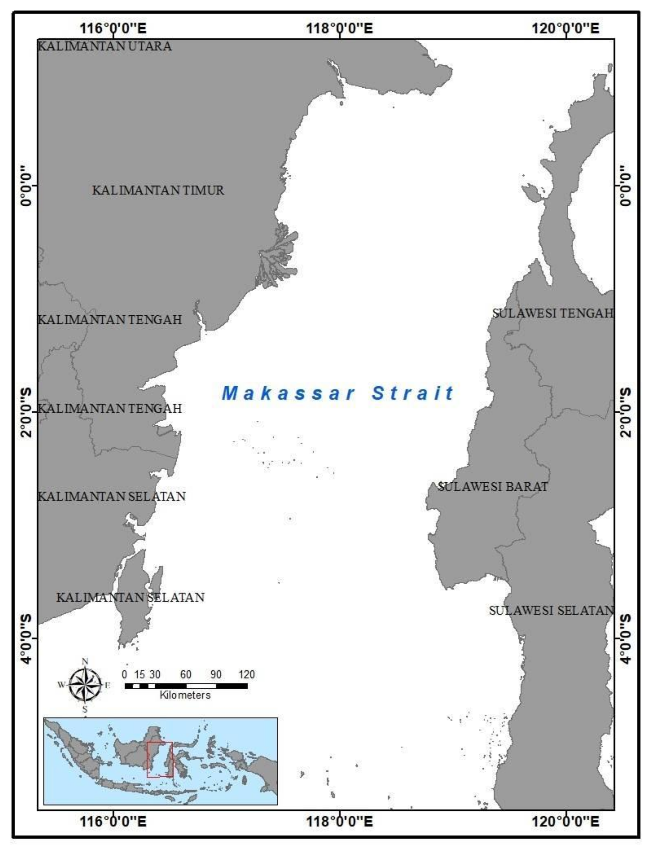
2.1. Study Area

The study area was located in the MS area with coordinates 1 N-5 S and 115–121 E. The area was selected based on oceanographic dynamics and the potential of the Makassar Strait in capturing fisheries based on Fisheries Management Area (FMA) 713 as shown in Figure 1.

In the 0° latitude area including the MS, several parameters such as monsoon, sea-level differences, and local wind affect its water characteristics [21]. The MS, as the main entrance of ITF, has a depth of around 1500 m that separates Borneo and Sulawesi [22]. The Makassar Strait is one of the most important and unique waters in Indonesia. The waters’ condition is influenced by both Kalimantan Island in the west and Sulawesi Island in the east. The MS is also known as one of the branches of the ITF that carries warm water masses from the Pacific Ocean to the Indian Ocean. It makes the character of the MS water very complex. Makassar Strait has a strong ocean current velocity with a dominant direction towards the south. The sea surface temperature of the northern part of the MS is warmer than the southern part and the sea level due to the confluence of two water masses [3].

2.2. Data

The data processing has a time span of 6 years, from 2015–2020. The data used are monthly spatial data. According to the study area, the Oceanographic data were cropped and processed using spatial software (

Table 1. Summary of specification of oceanographic parameter data and Eastern Little Tuna.

No.	Parameter	Sensor	Unit	Resolution		Sources
				Temporal	Spatial
1.	Sea Surface Temperature	AquaMODIS	°C	Monthly	4 km × 4 km	https://oceancolor.gsfc.nasa.gov (accessed on 8 August 2022)
2.	Chlorophyll-a	AquaMODIS	mg/m3	Monthly	4 km × 4 km	https://oceancolor.gsfc.nasa.gov (accessed on 8 August 2022)
3.	Sea Surface Salinity	SMAP	ppt	Monthly	40 km	https://marinecopernicus.eu (accessed on 8 August 2022)
4.	Current Velocity	CMES	m/s	Monthly	8 km	https://marinecopernicus.eu (accessed on 8 August 2022)
5.	Sea Surface Height	CMES	cm	Monthly	8 km	https://marinecopernicus.eu (accessed on 8 August 2022)
Fishery Data
No.	Parameter	Fishing Gear	Gross Toned (GT)		Sources
1.	Eastern Little Tuna	Purse Seine Gill Net	6–99		- Ministry of Marine Affairs and Fisheries, Marine and Fisheries Department of West Sulawesi

).

Image data from the Marine Copernicus website were downloaded after adjusting the coordinates. Meanwhile, image data from Ocean Color were downloaded directly. For the analysis, all the oceanographic data were composed into monthly data and resampled into 9 km spatial resolution. The image dataset was then cropped depending on the study area using ArcGIS. A cropping image dataset is a technique used to determine exactly which part of the image contains the object area to be processed [23].

2.2.1. Oceanographic Parameter Data Processing

The method used in this research is the remote sensing approach. The processed oceanographic parameter image data starts from 1 January 2015 to 31 December 2020. The data are processed temporally and spatially. Then spatial data processing is carried out by visualizing the data and functioning to extract oceanographic parameter values, which will then be processed by R language to develop GAM models used to predict fishing areas.

2.2.2. Eastern Little Tuna Data Processing

Catch data are expressed in CPUE (catch per unit effort). CPUE is a method to find out the ups and downs of fishery production, which are averaged annually and determined by the amount of spatial production. The calculation of CPUE using the equation:

$$\mathrm{CPUEi}=\frac{{\mathrm{Catchi}}_{\mathrm{i}}}{{\mathrm{Effort}}_{\mathrm{i}}}$$

where:

CPUEi = catch per fishing effort (kg/trip)

Catch_i = catch in year t (kg)

Effort_i = fishing effort in year t (trip)

Before calculating the CPUE, standardization of fishing gear is first carried out if more than one type of fishing gear is used. The Eastern Little Tuna (Euthynnus affinis) resources in the Makassar Strait are caught using gill nets and purse seines (PS = 1. GN = 0.63). The standardization of fishing gear is performed by calculating the average CPUE per fishing gear and the FPI (fishing power index) value.

$$\mathrm{FPI}=\frac{{\mathrm{CPUE}}_{\mathrm{I}}}{{\mathrm{CPUE}}_{\mathrm{S}}}$$

where:

FPI = Catching effort factor on the type of fishing gear

CPUE_i = Catch per annual fishing effort of other fishing gear (kg/trip)

CPUE_s = Catch per annual effort of standard gear (kg/trip)

These CPUE data are used to determine the yield of fishery production from water and develop a statistical approach to GAM using R software, which is then used to predict fishing areas.

2.2.3. Fishing Prediction Area Processing

GAM was made from the mgcv package using R software, with catch data as the response variable and SST, chlorophyll-a, salinity, current velocity, and SSHA as predictor variables. The equation used is:

$$g\left(\mu i\right)=b+s1\left(x1i\right)+s2\left(x2i\right)+s3\left(x3i\right)+\dots sn\left(xni\right)$$

where:

• g = link function
• i = response variable
• b = constant model
• x_n = developed parameter
• s_n = spline function smooth factor.

Model selection was based on significance of model term, reduction in Akaike’s Information Criterion (AIC), and increase in Cumulative Deviance Explain (CDE). The definition of AIC is a measure of goodness-of-fit as well as penalty on the number of model parameters. AIC can be calculated for each possible combination of explanatory variables, and the model with the lowest AIC is selected as the most optimal model [24]. The Cumulative Deviance Explained percentage measured how well the models fit the data [25].

A histogram represents the frequencies of values of variables bucketed into ranges. Each bar in histogram represents the height of the number of values present in that range. A histogram is made to determine the optimal parameter values in the tuna fishing area by looking at the relationship between the highest CPUE value and the range of oceanographic parameter values. They may be executed in an R session with the command:

$$\mathrm{hist}\left(\mathrm{formula}, \mathrm{xlab}=, \mathrm{ylab}=, \mathrm{main}=, \mathrm{col}=\right)$$

where:

• formula = a formula refers to the oceanographic parameters
• xlab = a character label for the x-axis
• ylab = a character label for the y-axis
• col = a string that indicates the color for the bars on the histogram

The function “predict.gam()” will add predicted values to the existing dataset. The command for predict function is:

$$\mathrm{predict}.\mathrm{gam}\left(\mathrm{object}, \mathrm{NewData}, \mathrm{type}=‘\mathrm{response}’\right)$$

where:

• object = a fitted ‘gam’ object as produced by ‘gam()’
• NewData = a data frame containing the values of the model covariates at which predictions are required
• type ‘response’ = to return predicted values on the same scale of the response you need to set.

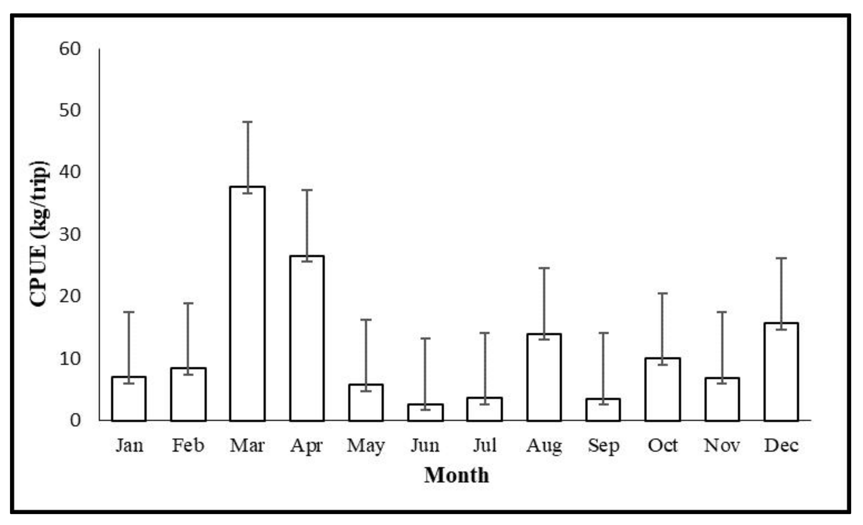
3. Results and Discussion

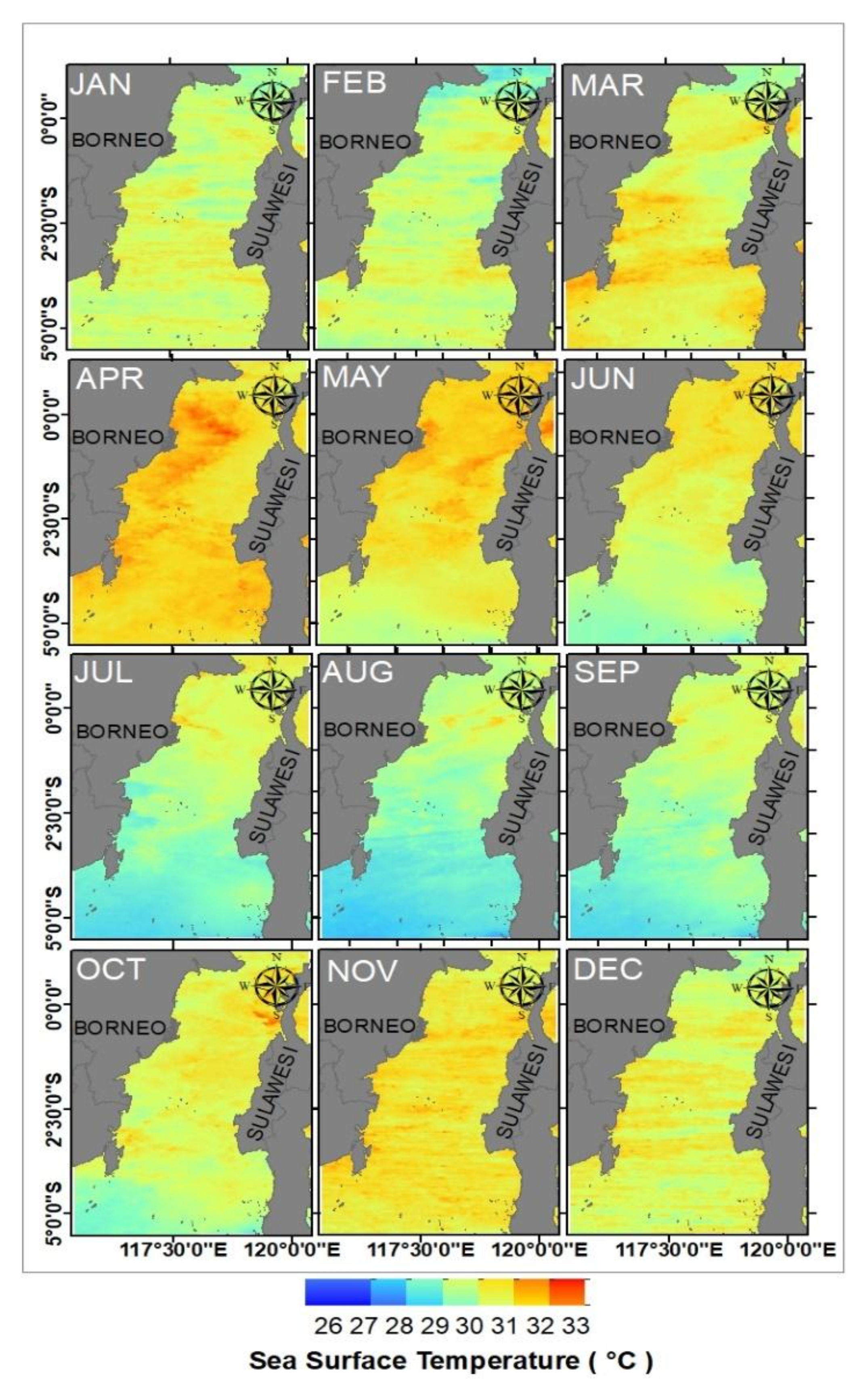
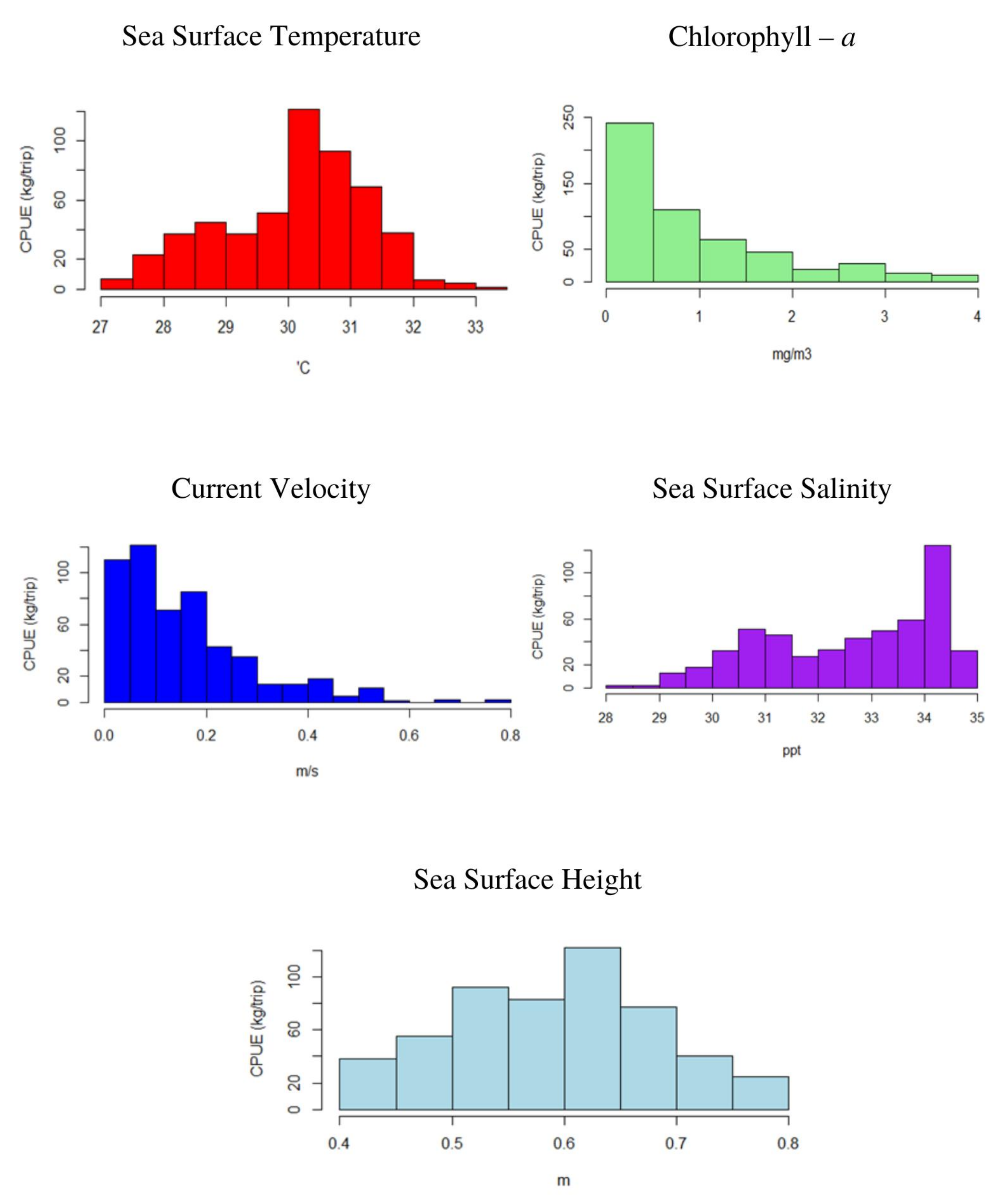
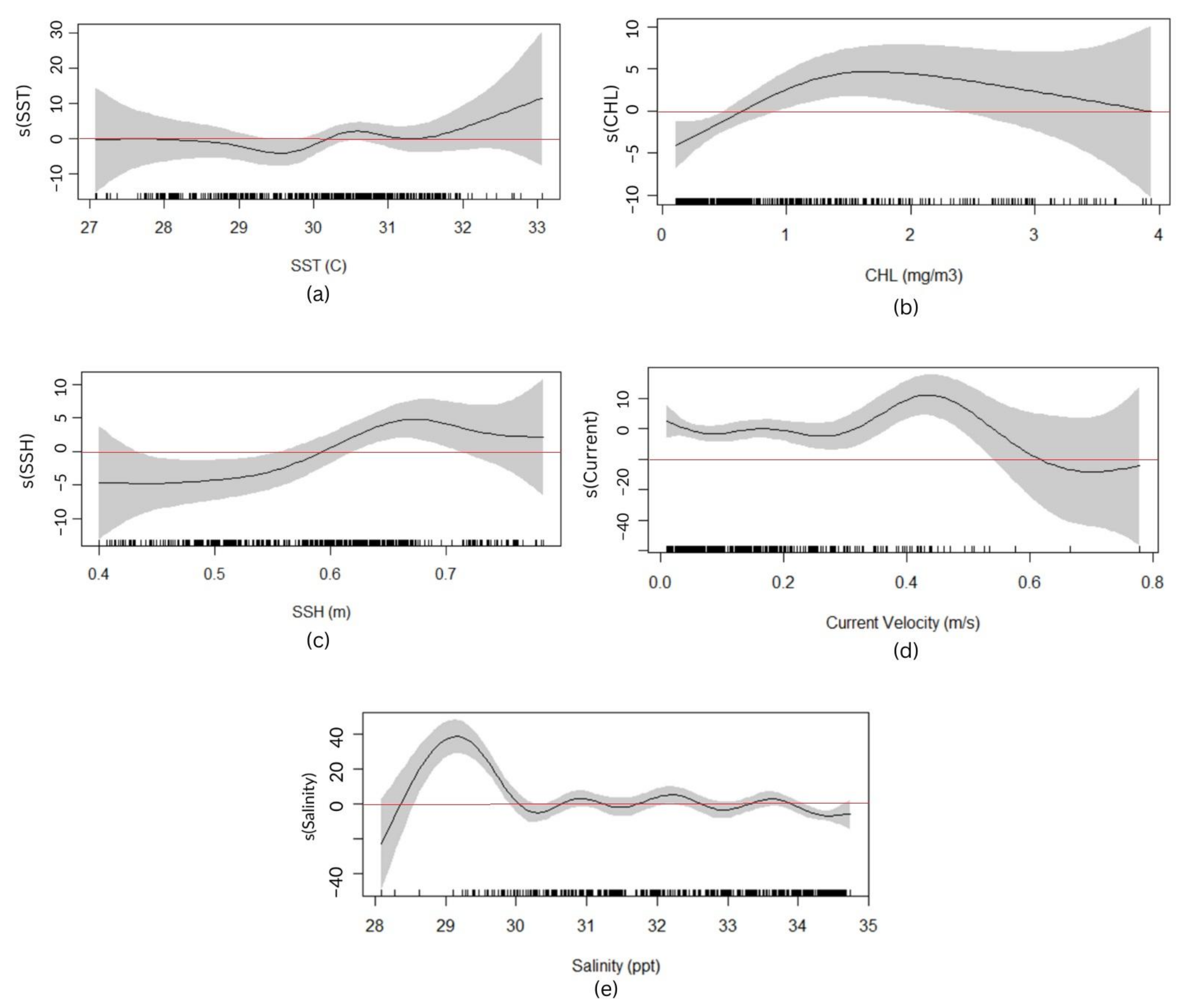
3.1. Sea Surface Temperature Variability

The seasonal pattern of the average sea surface temperature is shown in Figure 2. During 2015–2020, the average sea surface temperature ranges from 29–31 °C. The average value of the highest sea surface temperature occurs in April, with a temperature of 30.88 °C. Meanwhile, the lowest average sea surface temperature occurred in August, with a temperature of 29.13 °C.

During the northeast monsoon period, the distribution of sea surface temperature in the MS waters was high. It increased again specifically in April, especially in the western part of the MS. The temperature distribution ranged from 31–32 °C, with the highest peak in April. From June until September, the sea surface temperature decreases, and there is a difference between the northern and southern parts of the MS. The north part of the MS has a higher temperature than the south part. Then, in October, the distribution of sea surface temperatures increased again until December. The highest average sea surface temperature distribution occurs in April, while August has the lowest sea surface temperature distribution. The weakening of the seasonal wind speed in April makes solar radiation more effective, causing high sea surface temperatures in that month [26].

As a poikilometric biota, sea surface temperature can influence the geographic range of the Eastern Little Tuna involving related behavioral mechanisms, such as feeding activity [15]. Eastern Little Tuna prefer to live in warmer water, specifically 29–30 °C.

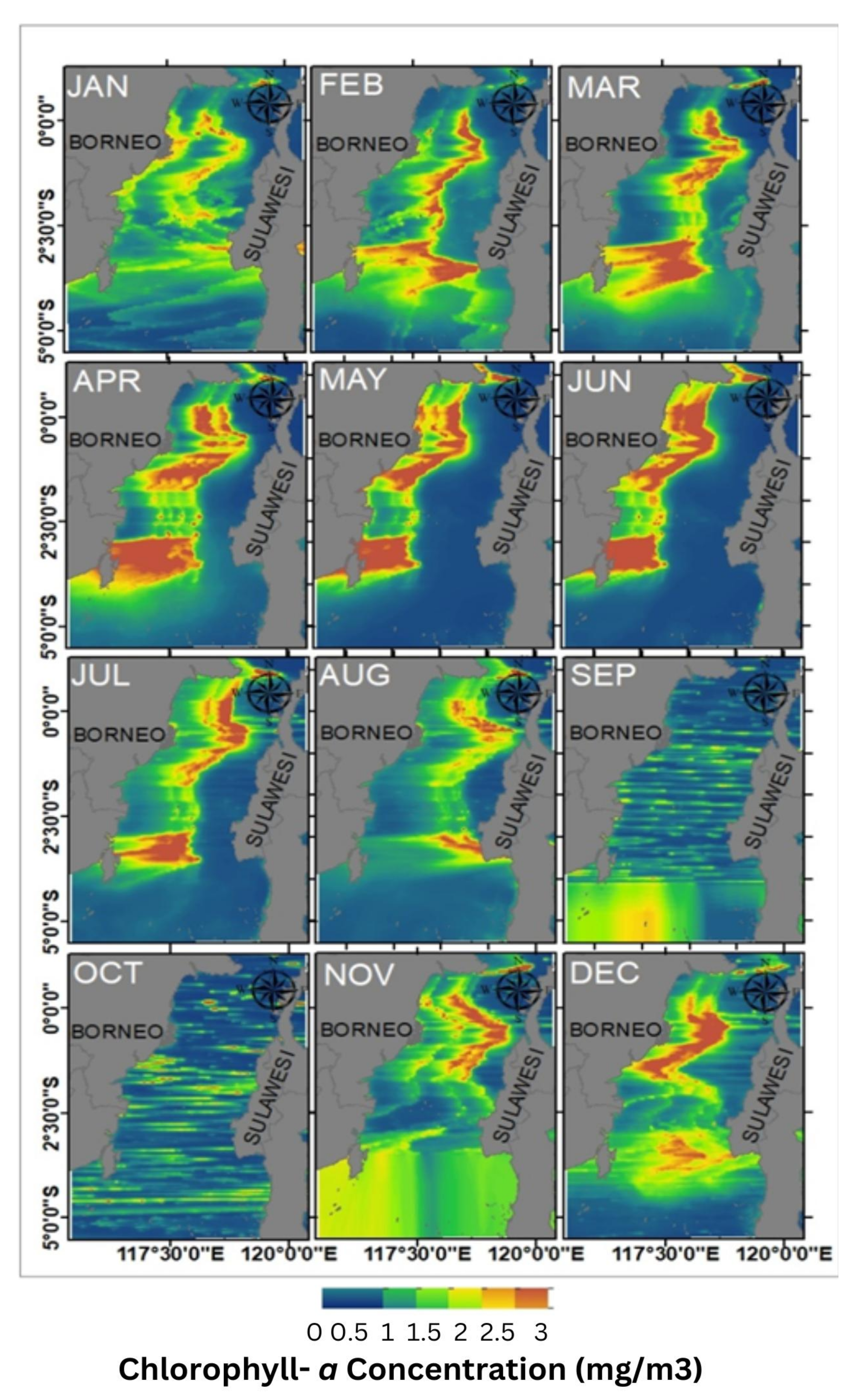
3.2. Chlorophyll-a Concentration Variability

The seasonal pattern of the average chlorophyll-a is shown in Figure 3. During 2015–2020, the average chlorophyll-a ranges from 0–3 mg/m³. The average value of the highest chlorophyll-a occurred in January at 0.65 mg/m^3, and the lowest average chlorophyll-a occurred in October with a concentration of 0.44 mg/m³.

The distribution of chlorophyll-a moves to the eastern part of the MS in the southeast monsoon with lower concentrations. Then, at the end of the northeast monsoon, the chlorophyll-a concentration again decreased with more even distribution throughout the waters. This means that this period has the lowest chlorophyll-a concentration. Meanwhile, the distribution of the highest concentration of chlorophyll-a occurred in December. Chlorophyll-a, which tends to increase from March to June, is caused by high rainfall, estimated to bring many nutrients from the mainland or the surrounding islands [27,28].

Chlorophyll-a concentration is an indicator of the biological productivity of water, and chlorophyll-a represents phytoplankton biomass [29]. The distribution state of chlorophyll-a concentration may be correlated with Eastern Little Tuna production; in other words, it can represent the productivity level of the coverage area. However, the number of fish in the water is not directly affected by the concentration of chlorophyll-a. The concentration of chlorophyll-a takes time before it is first consumed by herbivorous organisms such as zooplankton and then becomes a consumer for the producers of the trophic level above it [30].

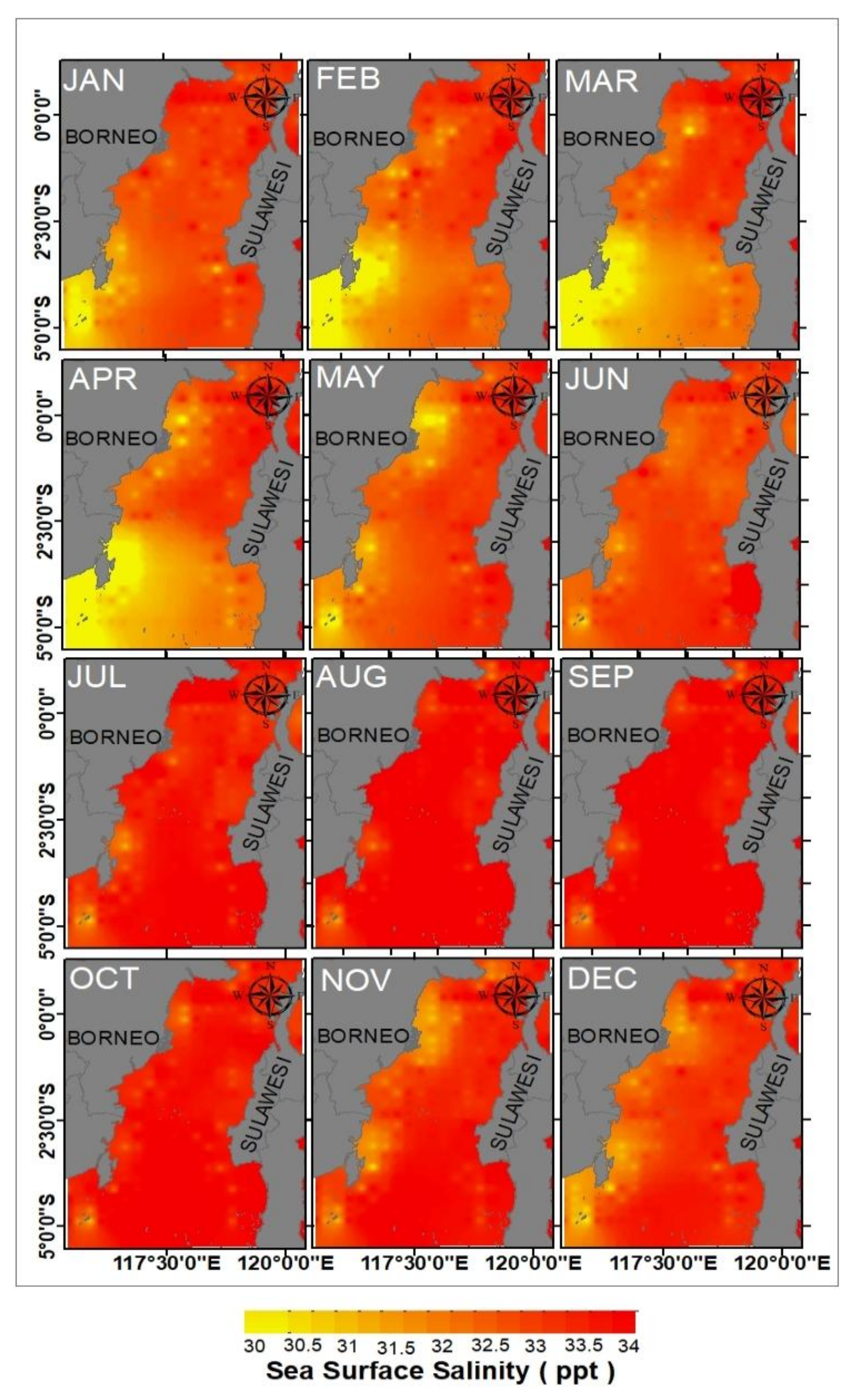
3.3. Sea Surface Salinity Variability

The seasonal pattern of the average salinity is shown in Figure 4. The average value of the highest salinity occurred in September with 33.64 ppt, and the lowest average occurred in March with a concentration of 32.28 ppt.

Based on the spatial distribution map of the average salinity in (Figure 4) in general, the salinity value in the MS waters in 2015–2020 has a pattern based on seasons. In the middle of the northeast monsoon in December, the average salinity value is high. Then from January until the beginning of the southwest monsoon (May), the average salinity value has lower value in the southern part than in the northern part of the MS. When the water mass with high salinity enters from the north of the MS, it prevents the lower-salinity water mass from the Java Sea from reaching the eastern part of the MS [31].

The wind carries low salinity surface waters of the Java Sea in southern Makassar Strait, creating a pressure gradient to the north in the surface layer of the strait. This “freshwater plug” inhibits the warm surface waters of the Pacific Ocean from flowing southward into the Indian Ocean, leading to a colder surface of the Indian Ocean [32]. In fish, salinity acts as a gas-liquid exchange system within the fish, affecting its metabolic system [33], and influencing migration patterns through which to find suitable salinity [34].

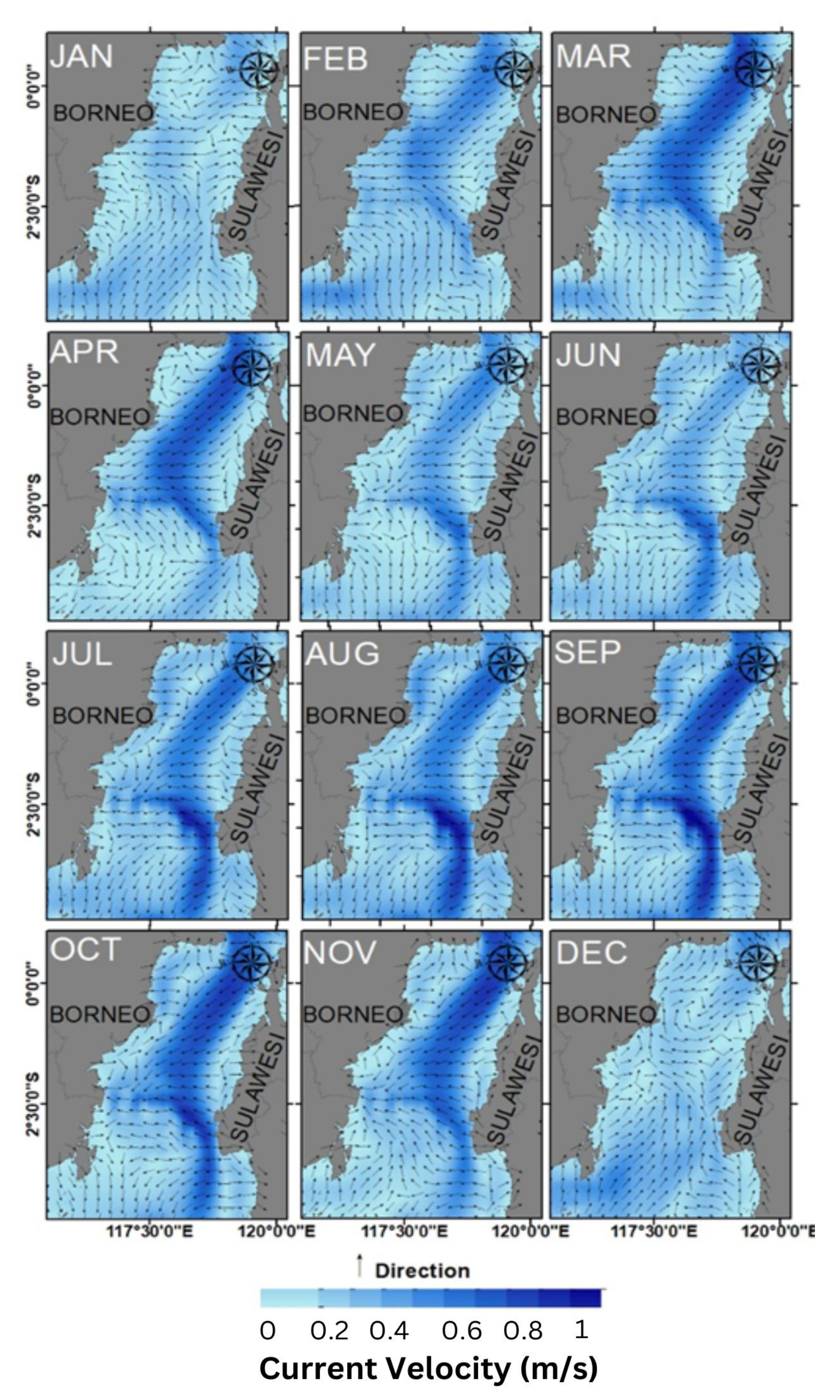
3.4. Ocean Current Direction and Velocity Variability

During 2015–2020, the average current velocity ranges from 0–1 m/s. The seasonal pattern of the average current direction and velocity is shown in Figure 5.

During the southwest monsoon, the average current velocity tended to be higher, with a range of 0.14–0.18 m/s. This value then decreased from December until February with a range of 0.12–0.17 m/s. Then, from June to August, the average current velocity increased at 0.14–0.18 m/s. At the beginning of the northeast monsoon (October to December), the average value of the current velocity was at 0.13–0.16 m/s, which is a decrease compared to the previous season.

Based on the map of the spatial distribution of the current direction and speed, the current velocity has the same pattern throughout the year. Ocean currents with a stronger velocity are from the northern part of the MS, originating from the Pacific Ocean. The pattern of current velocity formed is marked with a dark blue color, representing the MS as one of the ITF branches. Ocean currents drive the distribution of nutrients and chlorophyll-a in response to water mass movements [35]. As a result, the presence of fish, including Eastern Little Tuna (Euthynnus affinis) is affected by the current direction.

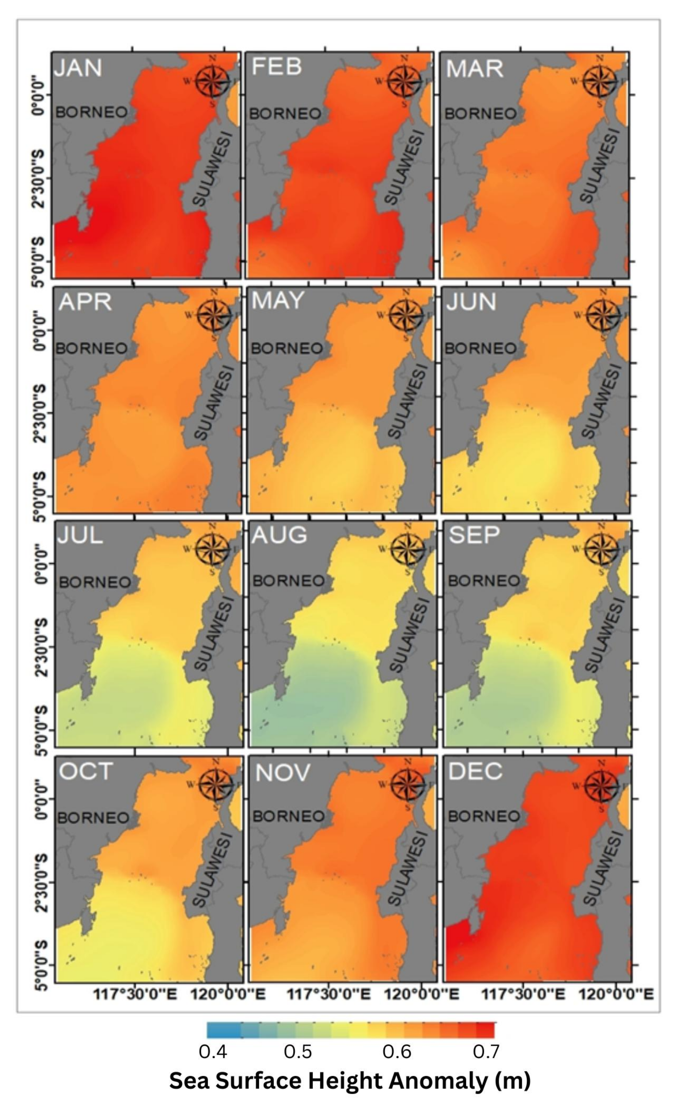
3.5. Sea Surface Height Variability

During 2015–2020, the average SSH ranges from 0.4–0.6 m. The seasonal pattern of the average SSH is shown in Figure 6. The average value of the highest SSH occurred in January at 0.68 m, and the lowest average occurred in August at 0.52 m.

In January, the red gradient means the sea level anomaly is at a high number of 0.7 m. From February until May, the sea level anomaly decreased. The sea level anomaly is low in the east monsoon, with differences in sea level in the north and south of the MS. The same thing happened until the middle of transitional season II. Then, the sea level anomaly increased in November with an average distribution of 0.56 m. The sea level anomaly increased again in December, with a figure of 0.64 m. The difference in sea level in the waters of the MS is caused by the difference in pressure between the two water masses originating from the Pacific Ocean and the Indian Ocean. The difference in sea level is at its maximum point during the east monsoon period until the beginning of the transition season (May to September) when the southeast monsoon occurs [36].

In general, the highest CPUE value occurred from March until May as shown in Figure 7. Meanwhile, the southwest monsoon was the seasonal period with the lowest CPUE value. The highest CPUE value was obtained in the end of the northeast monsoon, with an average CPUE value of 11.9–67.4 kg/trip. The lowest CPUE value was obtained at the southwest monsoon, with numbers ranging from 2.6–10.5 kg/trip. The relation between the catch CPUE of Eastern Little Tuna and oceanographic parameters is shown in Figure 8.

The relationship between the CPUE value of Eastern Little Tuna (Euthynnus affinis) and oceanographic parameters during 2015–2020 is presented in the form of a histogram (Figure 8). The histogram was formed to determine the optimal oceanographic parameter values in the Eastern Little Tuna fishing area by looking at the relationship between each parameter’s highest CPUE value and the range of values. The highest CPUE value was obtained at sea surface temperature values of 30–30.5 °C with an accumulated CPUE value of 120 kg/trip. The highest CPUE accumulation value of 250 kg/trip was obtained at the chlorophyll-a concentration value of 0.1–0.5 mg/m³. The highest CPUE accumulation value of 120 kg/trip was obtained at a salinity value of 34–34.5 ppt. The highest CPUE value was obtained at the current speed of 0.05–0.1 m/s. Then, the highest CPUE value was obtained at sea level at 0.6–0.65 m.

The relationship between the catch of Eastern Little Tuna (Euthynnus affinis) and oceanographic parameters can be determined using the Generalized Additive Model (GAM) statistical modeling analysis. The GAM model is formed with one response variable followed by a combination of two, three, to five predictor variables. The response variable used is the CPUE value of Eastern Little Tuna (Euthynnus affinis), while the explanatory variables used include sea surface temperature, chlorophyll-a, salinity, sea level, and current speed. Of the five variables, 26 prediction models were formed as shown in

Table 2. GAM-derived Deviances and AIC Values.

Models	Variables	p-Value	AIC	CDE (%)
$\mathrm{Sal}$	Salinity	<2.00 × 10−16 ***	4652.5	14.6
$\mathrm{SSH}$	SSH	0.00351 **	4706.9	3.52
$\mathrm{Arus}$	Current	0.0482 *	4652.5	3.29
$\mathrm{Chl}$	Chl	0.00659 **	4709.4	2.64
$\mathrm{SST}$	SST	0.00181 **	4711.07	1.82
$\mathrm{SST}+ \mathrm{Sal}$	SST Salinity	0.4 <2.00 × 10−16 ***	4653.31	16.2
$\mathrm{Chl}+\mathrm{Sal}$	Chl Salinity	0.721 <2.00 × 10−16 ***	4654.17	14.7
$\mathrm{SSH}+\mathrm{Sal}$	SSH Salinity	0.575 <2.00 × 10−16 ***	4654.21	14.6
$\mathrm{Arus}+\mathrm{Sal}$	Current Salinity	0.686 <2.00 × 10−16 ***	4654.39	14.6
$\mathrm{SSH}+\mathrm{Arus}$	SSH Current	0.0202 * 0.2082	4706.13	5.78
$\mathrm{Chl}+\mathrm{Arus}$	Chl Current	0.00431 ** 0.0498 *	4704.3	5.64
$\mathrm{Chl}+\mathrm{SST}$	Chl SST	0.049 * 0.215	4708.14	4.58
$\mathrm{SST}+\mathrm{Arus}$	SST Current	0.00152 ** 0.0637 *	4706.64	4.53
$\mathrm{SST}+\mathrm{SSH}$	SST SSH	0.2219 0.0974 *	4707.4	3.76
$\mathrm{SST}+ \mathrm{SSH}+\mathrm{Sal}$	SST SSH Salinity	0.423 0.711 <2.00 × 10−16 ***	4655.14	16.2
$\mathrm{Chl}+\mathrm{SST}+\mathrm{Sal}$	Chl SST Salinity	0.828 0.409 <2.00 × 10−16 ***	4655.21	16.2
$\mathrm{SSH}+\mathrm{Arus}+\mathrm{Sal}$	SSH Current Salinity	0.577 0.689 <2.00 × 10−16 ***	4656.07	14.7
$\mathrm{Chl}+\mathrm{SST}+\mathrm{Arus}$	Chl SST Current	0.0515 * 0.1637 0.0555 *	4703.4	7.31
$\mathrm{SST}+\mathrm{SSH}+\mathrm{Arus}$	SST SSH Current	0.416 0.284 0.174	4707.29	6.39
$\mathrm{SST}+\mathrm{CHL}+\mathrm{Arus}$ $+\mathrm{Sal}$	SST SSH Current Salinity	0.347 0.717 0.384 <2.00 × 10−16 ***	4659	16.3
$\mathrm{SST}+\mathrm{SSH}+\mathrm{Arus}$ $+\mathrm{Sal}$	SST SSH Current Salinity	0.372 0.837 0.445 <2.00 × 10−16 ***	4656.58	16.3
$\mathrm{Chl}+\mathrm{SST}+\mathrm{SSH}$ $+\mathrm{Sal}$	Chl SST SSH Salinity	0.821 0.429 0.707 <2.00 × 10−16 ***	4657.04	16.2
$\mathrm{Chl}+\mathrm{SSH}+\mathrm{Arus}$ $+\mathrm{Sal}$	Chl SST SSH Salinity	0.673 0.583 0.609 <2.00 × 10−16 ***	4657.6	14.8
$\mathrm{Chl}+\mathrm{SST}+$ $\mathrm{SST}+\mathrm{Arus}$	Chl SST SSH Current	0.102 0.457 0.575 0.104	4704.5	7.74
$\mathrm{CHL}+\mathrm{SST}+\mathrm{CHL}$ $+\mathrm{Arus}+\mathrm{Sal}$	CHL SST SSH Current Salinity	0.374 0.719 0.839 0.417 <2.00 × 10−16 ***	4658.36	16.4

. Of all the models developed, the model with the highest potential was determined by looking at the results of Akaike’s Information Criterion (AIC) [37] and Cumulative Deviance Explained (CDE). The model with the lowest AIC value and the highest CDE has the highest level of accuracy in explaining the response variable [24].

The model with a combination of five parameters (chlorophyll-a, sea surface temperature, salinity, sea level, and currents) has the smallest AIC value with the largest CDE. This shows that the model is a model with the highest potential to determine fish catches. The CDE value obtained from this model is 16.4%. The parameter that positively affects the catch of Eastern Little Tuna based on the GAM model form is salinity. This can be seen from the significance value <2.00 × 10⁻¹⁶. The salinity significance value obtained is close to zero. Meanwhile, the sea level parameter is the parameter with the lowest potential for the catch. The significance value obtained by sea level is 0.839.

A significant relationship between salinity parameters and catch results occurs because it follows the statement of Potier, 1998 in Amri (2017) that changes strongly influence the presence of pelagic fish in the spatial distribution of salinity [38]. This is also supported by Gunarso’s (1985) statement, which states that tuna is very sensitive to changes in salinity. Salinity is an oceanographic parameter that plays a direct role in fish movement [39].

Salinity greatly affects the process of osmoregulation of marine life, especially fish. Eastern Little Tuna (Euthynus affinis) tend to prefer waters with salinity that is more compatible with their body’s osmotic pressure. Changes in salinity will stimulate fish to migrate to areas where salinity matches the osmotic pressure of the body [40].

The chlorophyll-a parameter became the following parameter that had a significant relationship with the catch with a significance value of 0.374. Abundant concentration in water causes an increase in plankton productivity, and then fish productivity will be influenced by the formed food chain [41]. The low significance value occurs because chlorophyll-a takes time or time lag for large fish species.

Compared with previous research in different areas [14], the study found that of the three parameters used (SST, Chl-a, and SSHA) chlorophyll-a was the parameter that most influenced the production of Eastern Little Tuna in West Java waters. The Eastern Little Tuna catch peaks during the transition season from southeast to northwest monsoon and decreases during southeast monsoon. The GAM results confirmed that chlorophyll-a appeared to be one of the major factors explaining variability in the study area.

Furthermore, the smoothing curve is the result of the smoothing curve function when forming the GAM model as shown in Figure 9. This function aims to model the relationship between the response variable and the predictor or explanatory variables.

If the GAM function developed is above the red line or the zero axis, the percentage value is higher, indicating a strong influence of these parameters. On the other hand, if the GAM function is below the zero axis, it demonstrates that the effect of these parameters on Eastern Little Tuna (Euthynnus affinis) is weak. From the GAM plot formed, the range of explanatory variable values can have a positive influence on the response variable. The positive effect obtained was used to determine the range of explanatory variables preferred by Eastern Little Tuna (Euthynnus affinis). The positive effect for the salinity parameter is in the range of 29–30 ppt. Then, the positive effect of chlorophyll-a ranged from 1–2 mg/m³.

The prediction carries out the potential fishing zone prediction for the little “tuna.gam” function in the R software. The data used as the basis or input in this process are monthly data from the same data as the GAM analysis process. The output data from this prediction follow the information, namely in the form of possible CPUE values obtained. The prediction map presented is the probability of obtaining the CPUE value in each season, overlaid with the actual CPUE value in the same period. This is to determine the suitability of the predicted model.

The average production yield and the highest CPUE value for Eastern Little Tuna (Euthynnus affinis) occurred in the southwest during the period of 2015–2020 as shown in Figure 10a–f. Based on predictions, catches will be at their maximum value if carried out in the southwest with fishing locations throughout the waters for March and April. Meanwhile, for May high CPUE values will be generated from Sulawesi waters. The color bar in the image represents the predicted CPUE value for Eastern Little Tuna. Based on the prediction results, the possible CPUE value obtained in the transitional season was around 17.5–25 kg/trip (Figure 10). In the northeast monsoon, the CPUE value obtained is in the range of 15–17.5 kg/trip. Furthermore, the east monsoon is the season period with the lowest possible CPUE value, between 10 kg/trip and 15 kg/trip. The possible CPUE values obtained at the end of the southwest monsoon are in the range of 10–17.5 kg/trip.

The five-parameter combination model is the best fitting model based on the AIC and CDE values. The model is then used as a formula to predict fishing catch result, which are then visualized spatially. The spatial and temporal distribution results of the data show the corresponding values; the most suitable season in terms of catch results and oceanographic variability parameters is March to May. Continuing this is supported by histogram fit with visualization of the formed prediction result (Figure 8). Statistical analysis showed a very clear relationship between Eastern Little Tuna catches and all oceanographic parameters. Fish resource management is regulated in Permen KP No.22/2021, including the estimation of fish resources and the environment of fish resources. One of the most important opportunities to improve tuna fishery management is the adoption of harvest control measures [42]. One way to achieve this is by knowing and catching fish in the best season. Based on this research, the best time for catching Eastern Little Tuna is March to May.

4. Conclusions

Based on this discussion, it can be concluded that the relationship between optimum oceanographic parameters and the catch of Eastern Little Tuna (Euthynnus affinis) based on GAM analysis for the sea surface temperature is between 30–31 °C and the chlorophyll-a is between 1–2 mg/m³. Additionally, the optimum value for the salinity is 29–30 ppt, current velocity is 0.3–0.5 m/s, and sea-level is between 0.6–0.7 m. Based on the GAM model formed, the model with five variables (SST, chlorophyll-a, salinity, current, and TML) is the most suitable model for the prediction area for Eastern Little Tuna fishing with a Cumulative Deviance Explained value of 16.4%. Salinity in the waters of the Makassar Strait is the predictor variable with the highest influence on Eastern Little Tuna catches with a significance value of <2.00 × 16⁻¹⁰. Based on the prediction model and map, March to May is the season with the highest predicted CPUE value. In contrast, the southwest monsoon (June to August) is a seasoning period with the lowest CPUE value.

References

1. Ridha, M. Kajian Pendekatan Ekosistem Dalam Pengelolaan Perikanan Di Wilayah Pengelolaan Perikanan (Wpp) 571 Selat Malaka Provinsi Sumatera Utara. Geografi 2016, 8, 166–176. Available online: https://jurnal.unimed.ac.id/2012/index.php/geo/article/viewFile/5780/5176 (accessed on 17 October 2022).
2. Siregar, N.M.A.; Swastanto, Y.; Said, B.D. Fishery resources management in the Republic of Indonesia’s fishery management region 711 for the sustainable fishery resources control. J. Pertahanan 2019, 5, 19–33. [Google Scholar] [CrossRef]
3. Koeshendrajana, S.; Rusastra, I.W.; Martosubroto, P. Wilayah Pengelolaan Perikanan Negara Republik Indonesia (WPPNRI) 713: Gambaran Umum, Potensi dan Pemanfaatannya. Potensi Sumber Daya Kelaut. Perikanan. WPPNRI 2019, 713, 1–248. [Google Scholar]
4. Purba, N.P.; Pranowo, W.S.; Ndah, A.B.; Nanlohy, P. Seasonal variability of temperature, salinity, and surface currents at 0° latitude section of Indonesia seas. Reg. Stud. Mar. Sci. 2021, 44, 101772. [Google Scholar] [CrossRef]
5. Jufri, A.; Nur, M. Distribusi Spasial dan Temporal Arus Permukaan Laut di Selat Makassar Spatial and Temporal Distribution of Sea Surface Currents in the Makassar Strait Siganus. J. Fish. Mar. Sci. 2020, 1, 69–73. [Google Scholar]
6. Putri, A.R.S.; Zainuddin, M.; Musbir, M.; Hidayat, R.; Mustapha, M.A. Mapping potential fishing zones for skipjack tuna in the southern Makassar Strait, Indonesia, using Pelagic Habitat Index (PHI). Biodivers. J. Biol. Divers. 2021, 22, 3037–3045. [Google Scholar] [CrossRef]
7. Pratiwi, D. Pemetaan Zona Potensial Penangkapan Ikan Cakalang (Katsuwonus pelamis) Berbasis Data Citra Satelit dan Data Hasil Tangkapan Di Perairan Barru, Selat Makassar; Universitas Hasanuddin: Makassar, Indonesia, 2018. [Google Scholar]
8. Nurdin, S.; Mustapha, M.A.; Lihan, T.; Zainuddin, M. Applicability of remote sensing oceanographic data in the detection of potential fishing grounds of Rastrelliger kanagurta in the archipelagic waters of Spermonde, Indonesia. Fish. Res. 2017, 196, 1–12. [Google Scholar] [CrossRef]
9. Putri, A.R.S.; Zainuddin, M. Impact of Climate Changes on Skipjack tuna (Katsuwonus pelamis) catch during May–July in the Makassar Strait. IOP Conf. Ser. Earth Environ. Sci. 2019, 253, 012046. [Google Scholar] [CrossRef]
10. Solanki, H.U.; Bhatpuria, D.; Chauhan, P. Applications of generalized additive model (GAM) to satellite-derived variables and fishery data for prediction of fishery resources distributions in the Arabian Sea. Geocarto Int. 2015, 32, 30–43. [Google Scholar] [CrossRef]
11. Akhlak, M.A. Hubungan Variabel Suhu Permukaan Laut, Klorofil-a Dan Hasil Tangkapan Kapal Purse Seine Yang Didaratkan di TPI Bajomulyo Juwana, Pati. Manag. Aquat. Resour. J. 2015, 4, 128–135. [Google Scholar]
12. Patty, S.I. Distribusi Suhu, Salinitas dan Oksigen Terlarut Di Perairan Kema, Sulawesi Utara. J. Ilm. Platax 2013, 1, 148–157. [Google Scholar] [CrossRef] [Green Version]
13. Cahya, C.N.; Setyohadi, D.; Surinati, D. Pengaruh Parameter Oseanografi terhadap Distribusi Ikan. Oseana 2016, 41, 1–14. [Google Scholar]
14. Syamsuddin, M.; Sunarto; Yuliadi, L. Oceanographic factors related to Eastern Little Tuna (Euthynnus affinis) catches in the west Java Sea. IOP Conf. Ser. Earth Environ. Sci. 2018, 162, 012044. [Google Scholar] [CrossRef]
15. Zainuddin, M.; Saitoh, K.; Saitoh, S.-I. Albacore (Thunnus alalunga) fishing ground in relation to oceanographic conditions in the western North Pacific Ocean using remotely sensed satellite data. Fish. Oceanogr. 2008, 17, 61–73. [Google Scholar] [CrossRef] [Green Version]
16. Rajapaksha, J.K.; Nishida, T.; Samarakoon, L. Environmental preferences of yellowfin tuna (Thunnus albacores) in the northeast Indian Ocean: An application of remote sensing data to longline catches. Int. J. Fish. Aquat. Sci. 2013, 2, 72–80. [Google Scholar]
17. Siregar, E.S.Y.; Siregar, V.P.; Agus, S.B. Analisis daerah penangkapan ikan tuna sirip kuning Thunnus albacares di perairan sumatera barat berdasarkan model gam. J. Ilmu Teknol. Kelaut. Trop. 2018, 10, 501–516. [Google Scholar] [CrossRef]
18. Syamsuddin, M.L.; Saitoh, S.-I.; Hirawake, T.; Bachri, S.; Harto, A.B. Effects of El Niño–Southern Oscillation events on catches of Bigeye Tuna (Thunnus obesus) in the eastern Indian Ocean off Java. Fish. Bull. 2013, 111, 175–188. [Google Scholar] [CrossRef] [Green Version]
19. Swathi, B.; Swarnalatha, V.; Jogu, V. The Use of Generalized Additive Model (GAM) To Assess Fish Abundance and Spatial Occupancy in North-West Bay of Bengal. Int. J. Sci. Res. Sci. Technol. 2019, 17–28. [Google Scholar] [CrossRef]
20. Zuur, A.F.; Ieno, E.; Walker, N.; Saveliev, A.; Smith, G.M. Reviewer: Aaron Christ Alaska Department of Fish and Game Mixed Effects Models and Extensions in Ecology with R. JSS J. Stat. Softw. 2009, 32, 2–4. [Google Scholar]
21. Nuzula, F.; Syamsudin, M.L.; Yuliadi, L.P.S.; Purba, N.P.; Martono. Eddies spatial variability at Makassar Strait—Flores Sea. J. Phys. Conf. Ser. 2017, 755, 012079. [Google Scholar] [CrossRef]
22. Atmadipoera, A.; Molcard, R.; Madec, G.; Wijffels, S.; Sprintall, J.; Koch-Larrouy, A.; Jaya, I.; Supangat, A. Characteristics and variability of the Indonesian throughflow water at the outflow straits. Deep. Sea Res. Part I Oceanogr. Res. Pap. 2009, 56, 1942–1954. [Google Scholar] [CrossRef]
23. Yuhandri Perbandingan Metode Cropping pada Sebuah Citra untuk Pengambilan Motif Tertentu pada Kain Songket Sumatera Barat. Komtekinfo 2019, 6, 97–107. [CrossRef]
24. Zuur, A.F.; Leno, E.; Smith, G.M. Analysing Ecological Data; Springer: New York, NY, USA, 2007. [Google Scholar]
25. De Oliveira, A.M.B.; Binner, J.M.; Mandal, A.; Kelly, L.; Power, G.J. Using GAM functions and Markov-Switching models in an evaluation framework to assess countries’ performance in controlling the COVID-19 pandemic. BMC Public Health 2021, 21, 2173. [Google Scholar] [CrossRef]
26. Zulkhasyni, Z. Pengaruh Suhu Permukaan Laut Terhadap Hasil Tagkapan Ikan Cakalang Di Perairan Kota Bengkulu. J. Agroqua 2015, 13, 68–73. [Google Scholar]
27. Adnan. Analisis suhu permukaan laut dan klorofil—A data inderaja hubungannya dengan hasil tangkapan ikan tongkol (Euthynnus affinis) di Perairan Kalimantan Timur. J. Amanisal PSP FPIK Unpatti-Ambon 2010, 1, 1–12. [Google Scholar]
28. Putra, T.W.L.; Kunarso, K. Distribusi Suhu, Salinitas dan Densitas di Lapisan Homogen dan Termoklin Perairan Selat Makassar. Indones. J. Oceanogr. 2020, 2, 188–198. [Google Scholar] [CrossRef]
29. Gomez, F.; Montecinos, A.; Hormazabal, S.; Cubillos, L.A.; Correa-Ramirez, M.; Chavez, F.P. Impact of spring upwelling variability off southern-central Chile on common sardine (Strangomera bentincki) recruitment. Fish. Oceanogr. 2012, 21, 405–414. [Google Scholar] [CrossRef]
30. Girsang, H.S. Studi Penentuan Daerah Penangkapan Ikan Tongkol Melalui Pemetaan Penyebaran Klorofil-A Dan Hasil Tangkapan Di Palabuhanratu, Jawa Barat. Ph.D. Thesis, IPB University, West Java, Indonesia, 2008; 86p. [Google Scholar]
31. Murty, S.A.; Goodkin, N.F.; Halide, H.; Natawidjaja, D.; Suwargadi, B.; Suprihanto, I.; Prayudi, D.; Switzer, A.D.; Gordon, A.L. Climatic Influences on Southern Makassar Strait Salinity Over the Past Century. Geophys. Res. Lett. 2017, 44, 967–975. [Google Scholar] [CrossRef]
32. Gordon, A.L.; Susanto, R.D.; Vranes, K. Cool Indonesian throughflow as a consequence of restricted surface layer flow. Nature 2003, 425, 821–824. [Google Scholar] [CrossRef]
33. Karuwal, J. Dinamika Parameter Oseanografi Terhadap Hasil Tangkapan Ikan Teri (Stolephorus spp) Pada Bagan Perahu Di Teluk Dodinga, Kabupaten Halmahera Barat. Sumberd. Akuatik Indopasifik 2019, 3, 123–140. [Google Scholar]
34. Aryodhyo. Hasil Tangkapan Cakalang Indonesia. Prosiding Seminar Implementasi Nusantara Di Bidang Perikanan; IPB: Bogor, Indonesia, 2015. [Google Scholar]
35. Hidayah, G.; Wulandari, S.Y.; Zainuri, M. Studi Sebaran Klorofil-a Secara Horizontal di Perairan Muara Sungai Silugonggo Kecamatan Batangan, Pati. Bul. Oseanografi Mar. 2016, 5, 52–59. [Google Scholar] [CrossRef]
36. Hasanudin, M. Arus Lintas Indonesia (Arlindo). Oseana 1998, 23, 1–9. [Google Scholar]
37. Akaike, H. A New Look at the Statistical Model Identification. IEICE Trans. Fundam. Electron. Commun. Comput. Sci. 1974, E90-A, 2762–2769. [Google Scholar] [CrossRef] [Green Version]
38. Amri, K. Analisis hubungan kondisi oseanografi dengan fluktuasi hasil tangkapan ikan pelagis di selat sunda. J. Penelit. Perikan. Indones. 2017, 14, 55. [Google Scholar] [CrossRef]
39. Ningsih, R.K.; Syah, A.F. Karakteristik parameter oseanografi ikan demersal di perairan laut arafura menggunakan data penginderaan jauh. Juv. Ilm. Kelaut. Perikan. 2020, 1, 122–131. [Google Scholar] [CrossRef]
40. Yunus, F.; Zainuddin, M.; Farhum, S.A. Pemetaan Daerah Potensial Penangkapan Ikan Tongkol (Euthynnus sp) Di Perairan Selat Makassar. J. IPTEKS Pemanfaat. Sumberd. Perikan. 2019, 6, 1–20. [Google Scholar] [CrossRef]
41. Sadly, M.; Hendiarti, N.; Sachoemar, S.I.; Faisal, Y. Fishing ground prediction using a knowledge-based expert system geographical information system model in the South and Central Sulawesi coastal waters of Indonesia. Int. J. Remote. Sens. 2009, 30, 6429–6440. [Google Scholar] [CrossRef]
42. California Environmental Associates. Trends in Marine Resources and Fisheries Management in Indonesia. A 2018 Review; CEA: San Francisco, CA, USA, 2018; 146p. [Google Scholar]
Figure 1. A Map showing the study area in the Makassar Strait. MS is flanked by Borneo Island in the west and Sulawesi on the east side (gray colors).
Jmse 11 00165 g001
Figure 2. The Spatial Distribution Map of Average Sea Surface Temperature 2015–2020 in the Makassar Strait.
Jmse 11 00165 g002
Figure 3. The Spatial Distribution Map of Average Chlorophyll-a 2015–2020 in the Makassar Strait.
Jmse 11 00165 g003
Figure 4. The Spatial Distribution Map of Average Salinity 2015–2020 in the Makassar Strait.
Jmse 11 00165 g004
Figure 5. The Spatial Distribution Map of Average Current Direction and Velocity 2015–2020 in the Makassar Strait.
Jmse 11 00165 g005
Figure 6. The Spatial Distribution Map of Average Sea Surface Height 2015–2020 in the Makassar Strait.
Jmse 11 00165 g006
Figure 7. Little tuna (Euthynnus affinis) monthly CPUE chart in 2020. Error bars indicate standard deviation.
Jmse 11 00165 g007
Figure 8. Histogram showing the frequency of CPUE and oceanographic parameters. Here, the fish catch in kg/trip, SST in °C, Chl-a in mg/m3, SSS in ppt, Current velocity in m/s, and SSH in m.
Jmse 11 00165 g008
Figure 9. GAM-derived effect of the five oceanographic variables on CPUE, from the model constructed with: (a) SST, (b) Chlorophyll-a, (c) Current Velocity, (d) SSH, and (e) Salinity. The grey-shaded area indicates the 95% confidence intervals; the solid line shows the fitted GAM function, which describes a predictor variable’s effect on the response variable (CPUE). The rug plot on the x-axis shows the relative density of data points. Values of a predictor variable indicating a positive effect on CPUE were read as all values for which the fitted GAM function was above the zero axis (red line).
Jmse 11 00165 g009
Figure 10. The potential fishing zone distribution of Eastern Little Tuna (Euthynnus affinis) in the Makassar Strait in (a) 2015, (b) 2016, (c) 2017, (d) 2018, (e) 2019, and (f) 2020.
Jmse 11 00165 g010aJmse 11 00165 g010bJmse 11 00165 g010c