Incorporation of Deep Kernel Convolution into Density Clustering for Shipping AIS Data Denoising and Reconstruction

Abstract

Automatic Identification System (AIS) equipment can aid in identifying ships, reducing ship collision risks and ensuring maritime safety. However, the explosion of massive AIS data has caused increasing data processing challenges affecting their practical applications. Specifically, mistakes, noise, and missing data are presented during AIS data transmission and encoding, resulting in poor data quality and inaccurate data sources that negatively impact maritime safety research. To address this issue, a robust AIS data denoising and reconstruction methodology was proposed to realise the data preprocessing for different applications in maritime transportation. It includes two parts: Density-Based Spatial Clustering of Applications with Noise based on Deep Kernel Convolution (DBSCANDKC) and the reconstruction method, which can extract high-quality AIS data to guarantee the accuracy of the related maritime research. Firstly, the kinematics feature was employed to remove apparent noise from the AIS data. The square deep kernel convolution was then incorporated into density clustering to find and remove possibly anomalous data. Finally, a piecewise cubic spline interpolation approach was applied to construct the missing denoised trajectory data. The experiments were implemented in the Arctic Ocean and Strait of Dover to demonstrate the effectiveness and performance of the proposed methodology in different shipping environments. This methodology makes significant contributions to future maritime situational awareness, collision avoidance, and robust trajectory development for safety at sea.

1. Introduction

Maritime transportation presents a crucial role in international trade, accounting for more than 90% of global freight traffic [1,2]. Maritime safety has gained increasing attention under the surge of ultra-large ships and the occurrence of catastrophic maritime accidents. To improve navigation safety, the Automatic Identification System (AIS) equipment onboard ships becomes mandatory under the Safety of Life at Sea (SOLAS) by the International Maritime Organization (IMO). According to the regulation, all passenger and international ships with a gross tonnage of more than 300 GT have to be equipped with AIS equipment [3,4]. AIS equipment is an automatic tracking and reporting system for ship-to-ship and ship-to-shore communication. It involves not only static information (e.g., Maritime Mobile Service Identity (MMSI), ship type, length, and call sign) but also dynamic information (e.g., latitude, longitude, speed, and heading) [5,6]. AIS data are transmitted every 2 s to 10 s during the voyage. Along with the mandatory use of AIS equipment and Information and Communications Technology (ICT), AIS data is exploding, generating almost one trillion bits of data daily [7,8]. Up to now, AIS data has been widely used for ship trajectory compression, ship trajectory clustering, ship trajectory classification, abnormal ship trajectory identification, ship trajectory prediction [9,10], ship collision avoidance [11,12,13,14,15,16,17], maritime situational awareness, and other related research [18,19,20,21,22]. Such applications reveal the critical role that AIS data play in current international shipping context.

However, AIS data frequently encounter noise, incorrect data, missing data, and packet loss during creation, encoding, transmission, and decoding [23]. These problems pose enormous challenges to maritime knowledge discovery [24]. Specifically, the AIS data preprocessing are essential for guaranteeing and improving the quality of following applications. Therefore, there is an urgent need to find new solutions for AIS data denoising and reconstruction.

To address these issues, scholars have proposed various strategies for trajectory reconstruction and denoising [25,26,27,28]. Some employ the kinematic properties of AIS data to eliminate abnormal data, while others use clustering methods to achieve the goal of denoising. In addition, AIS data denoising and reconstruction methods based on deep learning have also exposed a rising profile, following the techniques of artificial intelligence and extensive data analysis [29]. Although showing some attractiveness, the existing AIS data denoising and reconstruction methods still reveal practical problems when being used to deal with the large size of big AIS data in investigated waters. This paper, therefore, aimed to solve the following research questions.

• Question 1: How to accurately handle noise, redundant, and abnormal data in big AIS data, relating to both large and small water areas?
• Question 2: How to reconstruct the trajectory after data denoising based on different ships?

This paper proposed a new holistic methodology for AIS data denoising, trajectory extraction, and reconstruction. The methodology consists of two parts: Density-Based Spatial Clustering of Applications with Noise based on Deep Kernel Convolution (DBSCANDKC) and a reconstruction method. Compared with the existing methods, the main contributions of this paper include:

(1)

Development of a systematical framework that enables rational AIS data denoising, trajectory extraction, and reconstruction.

(2)

Incorporation of deep kernel convolution and density clustering into the process of AIS data denoising.

(3)

Application of the piecewise cubic spline interpolation method in trajectory reconstruction, in which the position and speed of ships are taken into account in an interpolation process.

(4)

Implementation of the experiments to verify the effectiveness of the proposed methodology in both big and small waterways.

The paper is organised as follows. A literature review of the current research on denoising and reconstructing AIS data-based trajectories is presented in Section 2. Section 3 introduces the new framework construction, followed by a series of case studies and experimental results in Section 4. Finally, Section 5 summarises the findings and future development.

2. Literature Review

AIS data are one of the essential sources of ship trajectory data. Therefore, removing the noise from the raw AIS data is among the most important steps for maritime safety analysis and abnormal behaviour identification. Several approaches have been proposed in the literature for ship trajectory denoising and reconstruction. Generally, these methods are divided into the following categories: (1) those based on AIS data features, (2) those based on clustering, and (3) those based on deep learning models.

2.1. Research on Denoising Based on AIS Data Features

The kinematic information of AIS data is often used to find noises in AIS data. Qu et al. [30] applied Newton’s equation of motion with kinematic information from AIS data to determine speed, distance, and other indicators. Zhang et al. [31] exploited linear interpolation to delete noise from AIS data. The method is basic and straightforward but does not take into account curved trajectories. Zhang et al. [32] put forward a multi-regime vessel trajectory reconstruction model to eliminate anomalous AIS data using information such as speed, acceleration, and Rate of Turn (ROT). The curved trajectory noises are removed based on this model. However, this method is only verified by rectangular experiments on certain large ships, leaving its generality to be further explored. Rong et al. [33] introduced a probabilistic trajectory prediction model that can aid in decomposing ship motion into horizontal and vertical dimensions and handles raw AIS data in these dimensions. Furthermore, a Markov model was included in extracting ship trajectories to perform anomaly detection on AIS data [34]. Tong et al. [35] coupled Markov Chain with Grey prediction to increase the performance of the Markov model to remove anomalous data in curved channels. However, the Markov model method is unsuitable for long-term trajectory prediction, and the denoising effect is hence limited.

It is easy to understand and apply the denoising approach based on features to handle AIS data. However, denoising methods often fail when dealing with complex external variables, so they are more competent for the preprocessing of data denoising.

2.2. Research on Denoising Based on Clustering

The clustering methods are also applied to deal with abnormal AIS data. Researchers exploited specific aspects of AIS data to assess trajectory similarity in prior work on trajectory clustering [36]. Li et al. [37] employed a density-based clustering algorithm, Ordering Points to Identify the Clustering Structure (OPTICS), to remove abnormal data. However, this approach has bad performance while processing large volumes of trajectory data. Li et al. [38] proposed an Adaptive Douglas–Peucker (ADP) method to speed up similarity measurements between huge AIS trajectories, increasing classification and clustering accuracy. Qi et al. [39] utilised the spatial clustering method to analyse historical AIS data from ships to conduct data denoising and realise trajectory prediction, achieving the self-adaptation of parameters. Zhen et al. [40] proposed a hierarchical and k-medoids clustering technique to learn and model ship navigation behaviours in coastal seas, improving maritime situational awareness. However, it is time-consuming. Dobrkovic et al. [41] applied a genetic algorithm to accelerate the denoising of ship trajectory clustering. Gao et al. [42] developed a multi-step sub-trajectory clustering approach to better understand and explain ship behaviour patterns.

The denoising methods based on clustering methods can generally deliver good results for small AIS data due to their unsupervised features and no training set required. However, they reveal such weaknesses as difficult threshold setting, long data calculation time, and low adaptability from their previous applications.

2.3. Research on Denoising Based on Deep Learning

AIS data denoising approaches based on deep learning have attracted increasing attention in recent years due to the growing applications of neural network models. Usage of deep learning methods to mine AIS data has become a hotspot of maritime safety research. Chen et al. [43] utilised an artificial neural network (ANN) to predict and reconstruct ship trajectories by the kinematic information from AIS data. This method helps remove anomalous AIS data. However, overfitting always occurs in ANN modules, causing bad performance. Due to the drawbacks of the overfitting in an ANN model, Chen et al. [44] combined Ensemble Empirical Mode Decomposition (EEMD) with an ANN model to develop a new approach which significantly outperformed the traditional ANN model in traffic flow prediction. In addition, the method also supported the processing of other traffic data. It can improve the accuracy of AIS data, but the experiment is only verified by a scenario involving a short-term traffic flow. Tang et al. [45] designed a hybrid prediction model that classified the original traffic data using EEMD and Fuzzy C-means Neural Network (FCMNN). Compared with the standard ANN method, the FCMNN model trains and optimises the network, which can successfully identify noises in the original dataset. At the same time, scholars conduct the denoising of the more complex ship trajectories in the waterways based on deep learning methods [46]. Zhang et al. [47] obtained denoising features using a deep auto-encoder and used k-means to handle denoised trajectories. The accuracy of denoising is substantially improved compared with existing approaches, but the design of motion behaviour elements still needs to be improved. Liu et al. [15] introduced a deep temporal clustering method to remove noise data. This approach has a more obvious clustering effect but is less effective in low-noise situations.

The AIS data denoising methods based on deep learning are prevalent in the research of ship trajectories. However, the associated high hardware cost, complex model design, and other factors need to be better addressed to stimulate their widespread use.

3. Methodology

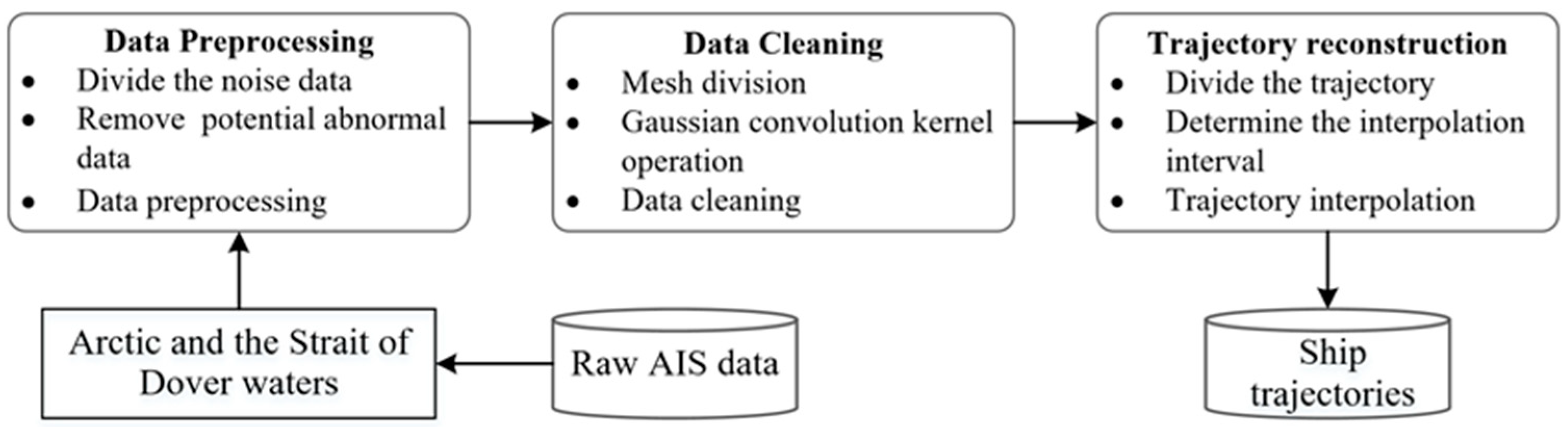
3.1. The Proposed Framework

This paper presented a solution to AIS data denoising, trajectory extraction, and trajectory reconstruction applications by the incorporation of deep kernel convolution into density clustering. It takes into account specific kinematic aspects in AIS data and overcomes many shortcomings of current AIS denoising methods. The flowchart of the proposed methodology is shown in Figure 1. Data collection and decoding can convert encoded data into ship static and dynamic information. Then, the trajectories are generated based on different ships. Trajectory preprocessing is carried out in three parts: ship trajectory division, extraction, and abnormal data cleaning. Furthermore, DBSCANDKC is conducted based on meshing, deep convolution kernel, and potential data cleaning. Finally, cubic spline interpolation is applied to construct the ship trajectories.

3.2. A New DBSCANDKC Method

Density-Based Spatial Clustering of Applications with Noise (DBSCAN) is a well-known method for grouping spatial data based on density [48]. Its essence is to separate the high-density and low-density areas, and then recognise noises. This method has two parameters to be set in advance: the number of points (MinPts) and a particular region (circular with radius Eps). The noises are that the density of the points is less than MinPts. Furthermore, this approach can locate clusters of various forms in noisy geographic datasets, identify noises, and remove anomalous data [49]. This paper proposes a new methodology to conduct data denoising, trajectory extraction, and trajectory reconstruction. DBSCANDKC can increase the denoising efficiency by converting the original circular neighbourhood in the classical DBSCAN into a 3 × 3 deep square convolution kernel with only one threshold MinPts. Therefore, only one parameter has to be set in it: the number of points covered by the square (a density threshold MinPts).

Given $G_{ij},i,j=1,2,\cdots ,N$ denotes the number of grids in the research areas, and MinPts is the threshold for each grid, the basic definition of DBSCANDKC is described in detail as follows.

Definition 1.

The density matrix consists of the number of data points in each grid and is shown below.

$$DM=\left[\begin{array}{ccc}{G}_{11}& \cdots & G_{1N}\\ ⋮& \ddots & ⋮\\ G_{N1}& \cdots & G_{NN}\end{array}\right]$$

(1)

Definition 2.

A deep convolution kernel is constructed by a dynamic Gaussian kernel function, and then used to perform the smoothing operation with the density matrix. The mathematical expression is shown below.

$$h(x)={\displaystyle \int f(x)g(x)dx}$$

(2)

where $h(x)$ is the feature map, $f(x)$ indicates the input information of the trajectory density matrix, and $g(x)$ denotes the Gaussian convolutional kernel. The schematic diagram of the Gaussian kernel convolution operation is presented in Figure 2.

Definition 3.

$N(G_i)$is the number of points in the 3 × 3 square convolution neighbourhood, which is defined by

$$N(G_i)=\{G_i=h(x_i)\},i=1,2,\cdots ,n$$

(3)

$p$is the core point when and only if$N(G_i)\ge MinPts$;

$p$is the noise point when it is not the core point.

3.3. The Proposed Methodology

The preliminary processing of original AIS data is to eliminate evident noise and anomalous data points based on kinematic features. Then, density clustering and deep convolution operation concepts are developed to handle some potentially aberrant data. After the grid meshing, the density matrix of AIS data points (i.e., $DM{1}_{N\times M}$) is generated to indicate the density distribution in the whole dataset. The dynamic and square convolution operation is conducted to obtain the new density matrix (i.e., $DM{2}_{N\times M}$) with a Gaussian kernel function. Then, the new trajectory dataset is obtained based on the $MinPts$ and square convolution. Finally, the trajectories are reconstructed to improve the quality of trajectories based on the piecewise cubic spline interpolation method. The flow of the proposed DBSCANDKC algorithm is shown in Algorithm 1.

Algorithm 1: DBSCANDKC
Input: Raw AIS trajectory dataset $data$ and density threshold $MinPts$
Output: The reconstructed trajectory dataset $Trdataset$
step 1	Get the ship AIS dataset $data1\leftarrow data(MMSI,Timestamp)$
step 2	Delete obvious abnormal data points and obtain the dataset     $data2\leftarrow data1\cap kinematicfeatures$     for $P_i$ in $data1$:       if $P_i.lon\in [-{180}^{\circ },{180}^{\circ }] \cap P_i.lat\in [-{90}^{\circ },{90}^{\circ }] \cap P_i.speed\in [1,40]$           $\cap item.course\in [0^{\circ },{360}^{\circ }] \cap d\in [0.05,1]$               $data2.reserve(P_i)$             else           $data2.noise(P_i)$       end if   end for
step 3	Grid meshing and generate density matrix $DM{2}_{N\times M}$     for $P_i$ in $data2$:         $DM1(i,j)\leftarrow P_i.lon\cap P_i.lat$     end for
step 4	Calculate the new density matrix $DM{2}_{N\times M}\leftarrow Deepconvolution(DM{1}_{N\times M})$
step 5	$data3\leftarrow \{DM2(i,j),MinPts\}$    for $DM2(i,j)$ in $DM{2}_{N\times M}$:       if $DM2(i,j)<MinPts$           $data3.noise(DM2(i,j))$     else           $data3.reserve(DM2(i,j))$      end if   end for
step 6	Ship trajectories $data4\leftarrow \{data3,MMSI,timestamp\}$
step 7	Reconstruct the trajectory data $Trdataset\leftarrow data4(cubicspline)$    for $P_i, P_{i+1}$ in $data4$:       if $|P_{i+1}.time-P_i.time| > 10 s$:              $Trdatase{t}_i\leftarrow cubicspline(P_i,P_{i+1})$        end if    end for
step 8	Return the reconstruct trajectories dataset $Trdataset$

3.3.1. Trajectory Preprocessing

The kinematic information is applied to delete the obvious error and noise data, such as abnormal latitude, longitude, course, and speed. The preprocessing steps are described as follows.

• Ship trajectory division;

MMSI is the unique identification number of ships, which can be used for the ship trajectory division. The ship data are separated based on different days. The timestamp and MMSI are combined to generate the new trajectory dataset.

• Abnormal Data Cleaning.

The latitude, longitude, course, and speed information are applied to remove the potential abnormal data.

The pseudocode of trajectory preprocessing is presented in Algorithm 2.

Algorithm 2: Trajectory preprocessing
Input: Raw AIS data $data$
Output: Preprocessed ship data $data2$
	for $P_i\in data$            $data1\leftarrow data(MMSI,Timestamp)$ split raw ship AIS data
	for $P_j\in data1$
	if $P_j.lon\notin [-{180}^{\circ },{180}^{\circ }] \left|\right| P_j.lat\notin [-{90}^{\circ },{90}^{\circ }]$
	or $P_j.speed\notin [1,40]$
	or $P_j.course\notin [0^{\circ },{360}^{\circ }]$
	or $d\notin [0.05,1]$
	continue
	else
	return $data2$ of the same MMSI on different days                 end if
	end for
	end for

3.3.2. Data Cleaning Based on Data Features and Deep Convolution

The denoising approach based on the kinematic information of AIS data can only eliminate evident erroneous data. Aberrant data needs to be further handled to generate cleaner data. The deep square kernel convolution operation with a dynamic Gaussian kernel function and density clustering are undertaken to discern the abnormal data. The steps are listed below.

• Mesh Division;

Build trajectory density matrix $DM{1}_{N\times M}$ based on latitude and longitude range.

• Convolution kernel operation;

When an AIS dataset is relatively large, the typical trajectory denoising approach (such as DBSCAN) will demand considerable memory support and I/O consumption, leading to bad performance and memory overflow. Therefore, this paper incorporated deep convolution-related notions into the AIS data denoising process in a novel way as follows.

Step 1. Reconstruct the density matrix.

Fill the boundary of the $DM{1}_{N\times M}$ with 0 and obtain a $\left(N+2\right)\times \left(M+2\right)$ density matrix.

Step 2. Build convolution kernel.

To verify the denoising performance of different convolution kernels, this study designes several convolution kernels, such as dynamic Gaussian kernel, mean convolution kernel, enhanced mean convolution kernel, and sharpening convolution kernel. The Radial Basis Function (RBF), commonly known as a Gaussian kernel function, is a radially symmetric scalar function. It can transform finite-dimensional data into high-dimensional space representation [50]. The most common definition is $k\left(\Vert x-x^{\prime }\Vert \right)$, which is the monotonic function of the Euclidean distance between every point $x$ in the space and a particular centre point $x^{\prime }$. The Gaussian kernel function can be defined as:

$$k\left(x,x^{\prime }\right)=e^{-\frac{\Vert x-x^{\prime }\Vert }{2{\sigma }^2}},$$

(4)

where $x^{\prime }$ is the centre of the kernel function and $\Vert x-x^{\prime }\Vert$ indicates the Euclidean distance between the vectors $x$ and $x^{\prime }$. The Gaussian kernel function in the procedure reduces monotonically as the distance between the two vectors grows. $\sigma$ controls the scope of the Gaussian kernel function. The larger the value, the more significant the local influence of the Gaussian kernel function.

Step 3. Convolution operation.

The 3 × 3 convolutional based on a dynamic Gaussian kernel function is carried out in the new $\left(N+2\right)\times \left(M+2\right)$ density matrix and the $N\times M$ density matrix $DM{2}_{N\times M}$ is obtained.

• Potential data cleaning.

The associated concepts of density clustering are applied in this paper to clean the potentially aberrant AIS data. Firstly, each element $DM{2}_{ij}$ of the density matrix $DM{2}_{N\times M}$ is compared to $DM{1}_{N\times M}$. Then, the threshold $MinPts$ is employed to remove the potential noises. The pseudocode of potential data cleaning is presented in Algorithm 3.

Algorithm 3: Potential Data Cleaning
Input: Density matrix $DM{1}_{N\times M}$, $DM{2}_{N\times M}$, and density threshold $MinPts$
Output: Kore points $data3$
	for $DM{2}_{ij}$ in $DM{2}_{N\times M}$:
	if $DM{2}_{ij}\le DM{1}_{ij}$
	$data3.noise(DM{2}_{ij})$
	else
	$data3.reserve(DM{2}_{ij})$          end if
	end for       return $data3$

3.3.3. Trajectory Reconstruction

Some data will inevitably be deleted during the data cleaning stage in real processing. It is necessary to reconstruct the trajectories. The trajectory reconstruction processing flow is presented in Algorithm 4.

• Ship trajectory division;

To complete the missing trajectory points more quickly and effectively, the new trajectory data $data3$ is needed to be split based on MMSI and timestamp. Then, the ship trajectories are separated to generate a new dataset.

• Determine the interpolation interval;

The original data were collected from satellite AIS data. There was much noise and missing data for a long period. Therefore, the time interval $T$ = 10 s was selected to determine the interpolation interval. If the time interval between the points $P_i$ and $P_{i+1}$ in the same trajectory is more than $T$, then the trajectory should be reconstructed. As a result, the data are interpolated using the points $P_i$ and $P_{i+1}$ as the starting and ending points.

• Trajectory interpolation.

Lagrange interpolation, piecewise linear interpolation, and cubic spline interpolation are the commonly used approaches for trajectory interpolation [51,52,53]. Cubic spline interpolation is a special case for the spline interpolation method. Compared with other interpolating polynomials, this approach generates a smoother interpolating polynomial with higher accuracy [54]. Therefore, the piecewise cubic spline interpolation approach is employed in this paper to improve the smoothness of the trajectories and the accuracy during trajectory reconstruction.

The speed of each trajectory point can be retrieved during the AIS data denoising. A function with time is applied to decompose the speed into longitude and latitude directions (i.e., $v_{lon}$ and $v_{lat}$) to express the information of each point. Furthermore, the integral operation is conducted on the spline function to obtain the $v_{lon}$ and $v_{lat}$. Finally, the information of each point is obtained at any time, including longitude, latitude, speed, and course. For any ship trajectory, the time $S_i(t)$ can be set in each sub-segment $Tr\left[t_i,t_{i+1}\right]$:

$$S_i(t_i)=v_{loni},S_i{}^{\prime }(t_i)={v^{\prime }}_{loni}=a_{loni},S_i{}^{\prime }(t_{i+1})={v^{\prime }}_{lon(i+1)}=a_{lon(i+1)},$$

(5)

Set the step size as $h_i=t_{i+1}-t_i$, $m_i=S_i(t)$, and then:

$$S_i(t)=c_i\left(\frac{t-t_i}{h_i}\right)v_{loni}+c_{(i+1)}\left(\frac{t-t_i}{h_i}\right)v_{lon(i+1)}+h_i{\delta }_i\left(\frac{t-t_i}{h_i}\right)m_i+h_i{\delta }_{(i+1)}\left(\frac{t-t_i}{h_i}\right)m_{(i+1)},$$

(6)

with $c_i(t)={(t-1)}^2(2t-1)$,

$$c_{(i+1)}(t)=t^2(-2t+3) c_i(t)=t^2(t-1),$$

(7)

Thus, a second-order derivative of Equation (5) gives:

$$\{\begin{array}{c}{S}_i(t_i)=6\times \frac{v_{lon(i+1)}-v_{loni}}{h_{\mathrm{i}}^2}-2\times \frac{2m_i+m_{i+1}}{h_i}\\ S_i(t_{i+1})=-6\times \frac{v_{lon(i+1)}-v_{loni}}{h_{\mathrm{i}}^2}+2\times \frac{2m_i+m_{i+1}}{h_i}\end{array},$$

(8)

To ensure the continuity of the two derivatives,

$$\frac{2m_i+m_{i+1}}{h_i}+\frac{2m_i+m_{i-1}}{h_{i-1}}=3\times \frac{v_{lon(i+1)}-v_{loni}}{h_i^2}+3\times \frac{v_{loni}-v_{lon(i-1)}}{h_{i-1}^2}$$

(9)

with ${\lambda }_i=h_{i-1}/{(h_{i-1}+h_i)}_i,g_i=3[(1-{\lambda }_i)(v_{loni}-v_{lon(i-1)})/h_{i-1}+{\lambda }_i(v_{lon(i+1)}-v_{loni})/h_i]$, then Equation (9) can be changed into:

$$(1-{\lambda }_i)m_{i-1}+2m_i+{\lambda }_i{m}_{i+1}=g_i,i=1,2,3,\cdots ,n-1,$$

(10)

For $\forall i$, there exists $m_i={v^{\prime }}_{\mathrm{l}oni}$, then

$$\{\begin{array}{c}2m_1+{\lambda }_1{m}_2=g_i-(1-{\lambda }_1){v^{\prime }}_{lon0}\\ \begin{array}{l}(1-{\lambda }_1)m_1+2m_2+{\lambda }_2{m}_3=g_2\\ \cdots \end{array}\\ (1-{\lambda }_{n-2})m_{n-3}+2m_{n-2}+{\lambda }_{n-2}{m}_{n-1}=g_{n-2}\\ (1-{\lambda }_{n-1})m_{n-2}+2m_{n-1}=g_{n-1}-{\lambda }_{n-1}{v^{\prime }}_{lonn}\end{array},$$

(11)

The system of equations can be rewritten as:

$$\left(\begin{array}{cccc}2& {\lambda }_1& & \\ 1-{\lambda }_1& 2& {\lambda }_1& \\ & \ddots & \ddots & \ddots \\ & 1-{\lambda }_{n-2}& 2& {\lambda }_{n-2}\\ 0& & 1-{\lambda }_{n-1}& 2\end{array}\right)\left(\begin{array}{c}\begin{array}{l}{m}_1\\ m_2\end{array}\\ ⋮\\ \begin{array}{l}{m}_{n-2}\\ m_{n-1}\end{array}\end{array}\right)=\left(\begin{array}{c}\begin{array}{l}{g}_i-(1-{\lambda }_1){v^{\prime }}_{lon0}\\ {\mathrm{g}}_2\end{array}\\ ⋮\\ \begin{array}{l}{g}_{n-2}\\ g_{n-1}-{\lambda }_{n-1}{v^{\prime }}_{lonn}\end{array}\end{array}\right),$$

(12)

Then, the coefficient matrix is obtained

$$M=\left(\begin{array}{cccc}2& {\lambda }_1& & \\ 1-{\lambda }_1& 2& {\lambda }_1& \\ & \ddots & \ddots & \ddots \\ & 1-{\lambda }_{n-2}& 2& {\lambda }_{n-2}\\ 0& & 1-{\lambda }_{n-1}& 2\end{array}\right).$$

(13)

Therefore, the segmented spline function solutions for $v_{lon}$ and $v_{lat}$ at the time $t$ can be solved. The associated latitude and longitude can be derived by integrating the speed in the longitude direction, realising the final goal of trajectory reconstruction.

Algorithm 4: Trajectory reconstruction
Input: Denoised AIS data $data3$
Output: Reconstructed trajectory data $Trdataset$.         Split $data3$            $data4\leftarrow \{data3,MMSI,timestamp\}$
	for $P_j$ in $data4$:
	if Δt > 10                     Reconstruct the trajectory data $Trdatase{t}_j\leftarrow data4(cubicspline)$              end if
	end for
	return $Trdataset$

4. Experimental Results and Analysis

4.1. Data Set and Experimental Design

To verify the effectiveness of the proposed methodology in trajectory denoising and reconstruction, experiments were implemented in the Arctic Ocean and the Strait of Dover water. The Arctic Ocean is large, with long transportation distances and many ports. Its complex navigational data is suitable for testing the performance of the proposed method when being required to cope with large areas. The Strait of Dover water is selected and used to demonstrate the robustness of the proposed method in a complex but small area. The details of original AIS data in the Arctic Ocean and the Strait of Dover water are listed in

Table 1. The data details for the two research study areas.

Water Areas	Time Span	Number of Trajectories	Number of Points	Longitude	Latitude
Arctic Ocean	1 September 2018–31 September 2018	108,588	53,267,239	170° W–180° E	66.089° N–90° N
Strait of Dover	1 January 2018–31 January 2018	3043	50,610	1.057° E–3.042° E	50.622° N–51.952° N

. As shown in Table 1, the original AIS information in the Arctic Ocean was collected from 1 September 2018 to 31 September 2018 with 108,588 ship trajectories with 53,267,239 points, while there were 3043 ship trajectories from 1 January 2018 to 31 January 2018 with 50,610 points in the Strait of Dover water.

The visualisation result of the original dataset in two water areas are shown in Figure 3 and Figure 4, respectively. It can be seen that there are apparent noises and abnormal data in the original AIS data. As aforementioned, the data denoising and reconstruction of large water areas are the research difficulties. The Arctic Ocean contains a large amount of AIS data that has to be processed.

All numerical experiments were performed using 64-bit Windows 10 on a 2.4 GHz Intel Core i5 9300H CPU, NVIDIA GeForce GTX 1650 GPU with 8 GB memory. The proposed algorithms were programmed in Python 3.9. The flowchart of experiments is shown in Figure 5.

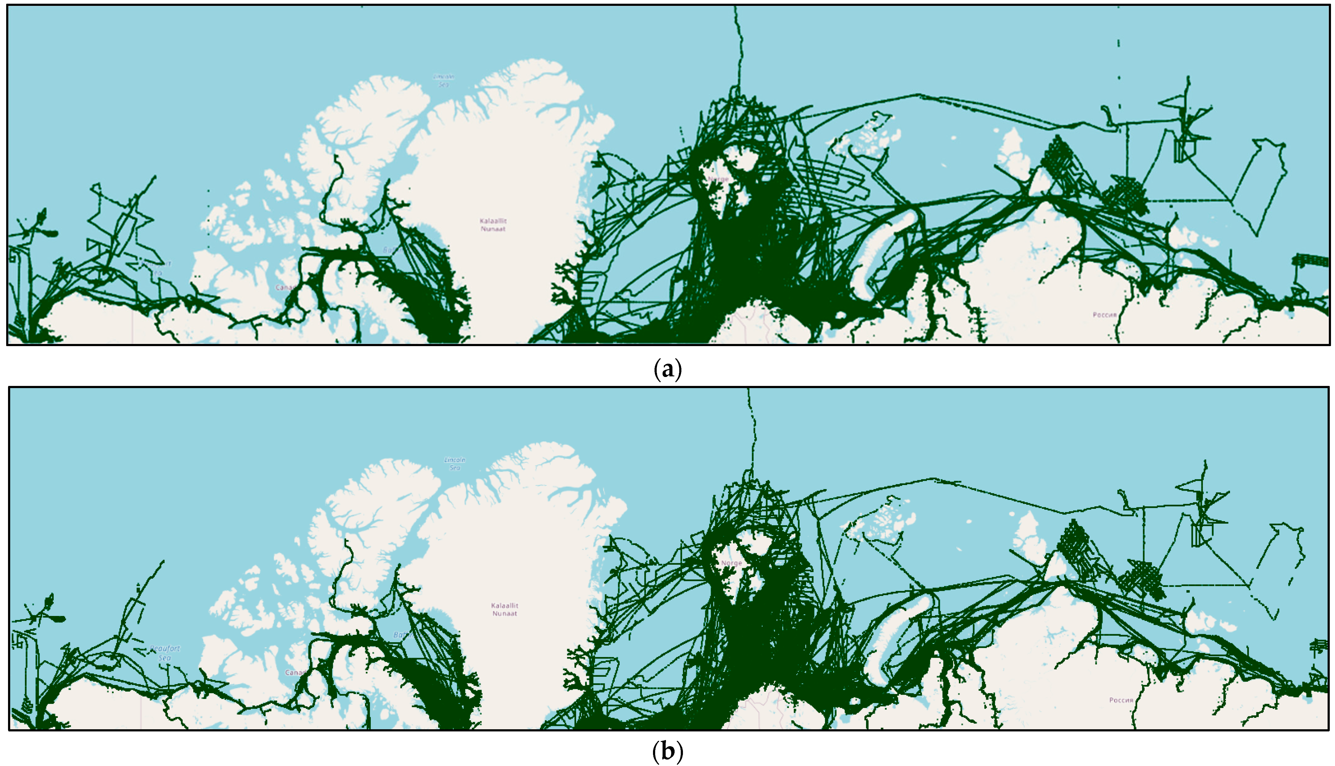
4.2. Visualisation Results of Different Kernel Functions

Three kinds of kernel functions were selected, and the results were compared to verify the effectiveness of the chosen Gaussian convolution kernel. They include a Gaussian convolution kernel function, mean convolution kernel function, and sharpening convolution kernel function. The visualisation results of the different kernel functions in the Arctic Ocean and the Strait of Dover water are shown in Figure 6 and Figure 7, respectively. The comparison results in Figure 6 and Figure 7 show that the performance of the Gaussian convolution kernel has the best performance. Therefore, the Gaussian kernel function is selected and applied to the trajectory denoising and reconstruction.

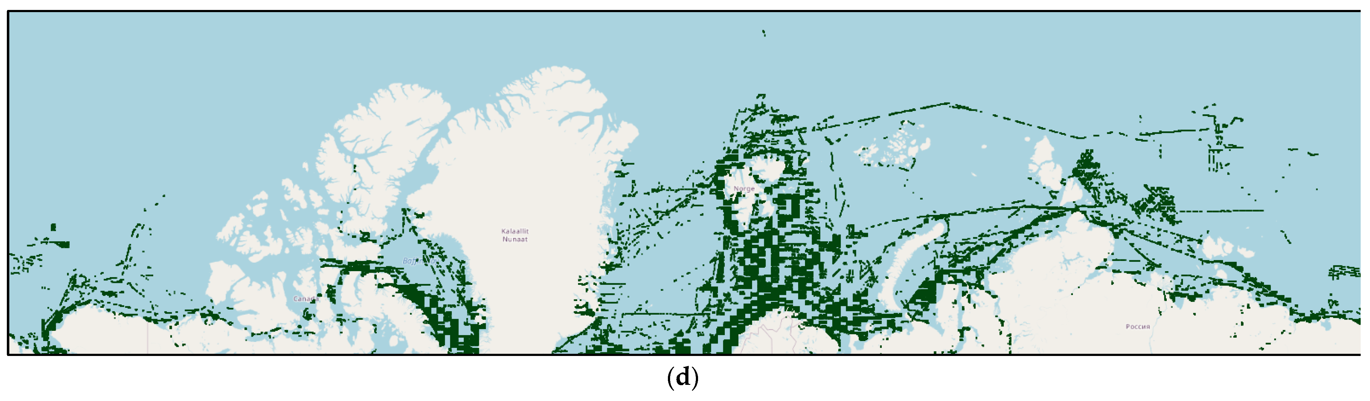
4.3. Visualisation and Analysis of Trajectory Denoising Results in Two Research Areas

To demonstrate the performance of the proposed DBSCANDKC method, the first experiment is carried out in a typical large area (i.e., the Arctic Ocean). The data preprocessing result in the Arctic Ocean is shown in Figure 8. Specifically, the results of simple data preprocessing, the deep convolution operation, and reconstruction trajectories are respectively displayed in Figure 8a–c. A 300 × 300 density matrix and a dynamic Gaussian convolution kernel are built to delete the possibly aberrant AIS data with $MinPts=5$. The number of data points and trajectory in the Arctic Ocean data preprocessing process are shown in

Table 2. The data and trajectory information on the Arctic Ocean.

	Raw Data Set	Dataset after Preprocessing	Dataset after Convolution	Dataset after Reconstruction
Trajectories	108,588	3046	2982	2982
Points	53,267,239	2,146,651	1,972,471	2,433,576

for comparison. It is evident that simple data preprocessing can delete the obvious noise data based on the results of Figure 3 and Figure 8a. Furthermore, the comparison of Figure 8a,b shows that the deep convolution operation can remove more abnormal data. As can be seen from Table 2, compared with the 108,588 trajectories with 53,267,239 points in the raw dataset, 3026 trajectories with 2,146,651 points are reserved after simple data preprocessing. Furthermore, there were 2982 trajectories with points after the deep convolution operation. The original dataset includes much of the data from all the waiting, berthing, and mooring ships. A lot of trajectories with anchorage points were removed. Eventually, the trajectory reconstruction was conducted to complete the trajectories, and there are 2982 trajectories with 2,433,576 points. The visualisation results of ship trajectories in the Arctic Ocean verified the performance of the proposed DBSCANDKC method.

The second experiment was carried out in a small and complex area, the Strait of Dover. The results of simple data preprocessing, the deep convolution operation, and reconstruction trajectories are displayed in Figure 9a–c, respectively. A $300\times 300$ density matrix and dynamic Gaussian convolution kernel were built to delete the possibly abnormal AIS data with $MinPts=3$. The data and trajectory information for denoising and reconstruction of the Strait of Dover are listed clearly in

Table 3. Information on the Strait of Dover water trajectories.

	Raw Data Set	Dataset After Preprocessing	Dataset after Convolution	Dataset after Reconstruction
Trajectories	3043	1057	1052	1504
Points	50,610	30,689	29,793	99,828

. It is evident that simple data preprocessing can delete the obvious noise data based on the results of Figure 3 and Figure 9a. Furthermore, the deep convolution operation can remove more abnormal data from Figure 9a,b. Compared to the 3043 trajectories with 50,610 points in the raw dataset, 1507 trajectories with 30,689 points are reserved after simple data preprocessing. Furthermore, there remaine 1504 trajectories with 29,793 points after the deep convolution operation. After the reconstruction, 1504 trajectories with 99,828 points are generated for future knowledge discovery. The experimental results show that the proposed methodology have better performance in trajectory denoising and reconstruction based on the comparative results of the Arctic Ocean and the Strait of Dover water.

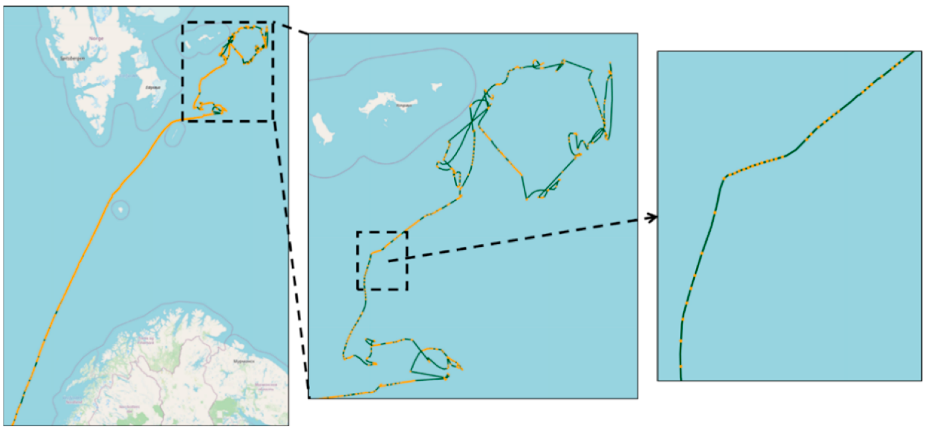
4.4. Trajectory Reconstruction and Comparative Analysis of Arctic Ocean

To further highlight the trajectory reconstruction performance of the proposed DBSCANDKC method in the Arctic Ocean, the ship trajectories with MMSI of 218832000 and 316025029 are selected as the real cases to deeply analyse the effectiveness.

The trajectory with MMSI 218832000 has 69,815 points, with the longitude range 1.553° E to 45.426° E and the latitude range 66.354° N to 82.558° N. Through experimental comparison and analysis, the denoising effect is the best when the size of the density matrix was set to 600 × 600 and $MinPts=3$ in the Arctic Ocean. The result during data denoising is shown in Figure 10. The trajectory information of MMSI 218832000 is shown in

Table 4. Trajectory information for different MMSIs.

MMSI	Raw Data Set	Dataset after Preprocessing	Dataset after Convolution	Dataset after Reconstruction
218832000	69,815	3815	819	3983
316025029	5215	3579	2142	4980
220002000	38	32	29	31
244554000	107	94	87	116

. Compared with 69,815 points in the raw dataset, 3815 points remained after simple data preprocessing. Furthermore, there are 819 points after the deep convolution operation. After the trajectory reconstruction, there are 3983 points. It is evident from the visualisation result that the proposed method had better denoising and reconstruction performance.

The interpolation result of the selected trajectory (MMSI 218832000) is displayed in Figure 11, where the orange points represent the raw ship AIS trajectory points, and the green lines represent the reconstructed trajectories. The trajectory of MMSI 218832000 has 5215 points, with the longitude range 115.2134° W to 61.015° W and the latitude range 66.342° N to 74.354° N. The visualisation result of trajectory reconstruction further verified the good performance of the proposed method.

To further show the effectiveness of the proposed method in a large area and the long trajectory, MMSI 218832000 is selected as a real case. It is a classical trajectory because it includes data in 23 days in the Arctic Ocean. The visualisation result of the data denoising process is shown in Figure 12. Firstly, the raw AIS trajectory is displayed in Figure 12a, which contains much noise data. The visualisation result after simple data preprocessing is presented in Figure 12b, and it seems that the performance was better. To have a clear insight into this trajectory reconstruction operation, the point data are visualised in Figure 12c. Finally, the reconstruction result is shown in Figure 12d to verify the necessity and effectiveness. Different colours represent the ship trajectories in 23 days.

The trajectory reconstruction result of the selected trajectory is displayed in Figure 13, where the orange points represent the raw ship AIS trajectory points, and the green lines indicate the reconstructed trajectories. Table 4 shows the trajectory information in each step of MMSI 316025029. Compared with the raw dataset with 5215 points, 3579 points remained after simple data preprocessing. Furthermore, there are 2142 points after the deep convolution operation. After the trajectory reconstruction, 4980 points are generated for future data mining. The visualisation results of the real cases demonstrated that the method had a good reconstruction effect under large water data sets and curved trajectories.

4.5. Trajectory Reconstruction and Comparative Analysis of Strait of Dover Waters

The case study in a small area is implemented in the two ship trajectories of MMSI 220002000 and MMSI 244554000 to demonstrate the performance of the proposed method. There are 38 points in the trajectory of MMSI 220002000, with a longitude range of 1.30° E to 1.85° E and a latitude range of 50.00° N to 51.26° N. The experimental comparison and analysis results showed that the denoising effect is the best when the size of the density matrix is set to 100 × 100 and $MinPts=2$. The result during data denoising is shown in Figure 14. The reconstruction result of the selected trajectory is displayed in Figure 15, where the orange points represent the raw ship AIS trajectory points, and the blue lines indicate the reconstructed trajectories. The trajectory information in each step is listed in Table 4. Compared with 38 points in the raw dataset, 32 points are reserved after simple data preprocessing. Furthermore, there are 29 points after the deep convolution operation. Eventually, 31 points are generated for future data mining after the trajectory reconstruction.

The trajectory with an MMSI of 244554000 has 107 points, with the longitude range 115.2134° W to 61.015° W and the latitude range 66.342° N to 74.354° N. Through experimental comparison and analysis, the denoising effect is the best when the size of the grid is set to 200 × 200 and $MinPts=3$. The result during data denoising is shown in Figure 16. The trajectory reconstruction result of the selected trajectory is compared in Figure 17, where the orange points represent the raw ship AIS trajectory points, and the blue line is the reconstructed trajectories. The trajectory information in each step is shown in Table 4. Compared with 107 points in the raw dataset, 94 points are reserved after simple data preprocessing. Furthermore, there are 87 points after the deep convolution operation. After the trajectory reconstruction, there are 116 points. As demonstrated by the experimental results, the method also had excellent reconstruction results under small waters and curved trajectories.

4.6. Discussion

The experimental results indicated that the methodology proposed in this paper had better AIS dada denoising and reconstruction effects in different waters. The proposed DBSCANDKC method had strong robustness both in large waters with massive data (such as the Arctic Ocean) and in small waters but with high traffic complications (such as the Strait of Dover water). Compared with the existing denoising methods based on clustering and deep learning models, it requires less memory while ensuring the denoising effect. The research results are committed to generating more accurate and high-quality AIS data for maritime safety management, thereby providing a reliable and robust foundation for subsequent research on maritime situational awareness, collision avoidance, route planning, etc. In terms of future studies, the proposed method takes into account the influence of latitude, longitude, and speed in the data preprocessing stage at present. To further improve the accuracy of the results, the impact of other factors (such as weather conditions, navigation of other ships, etc.) on AIS data could be further explored.

5. Conclusions

With the growing use of AIS data in maritime research, an emerging concern is rising as the explosion of AIS data has resulted in errors, redundancy, and noise in its generation and transmission. To address this problem, a new holistic methodology, DBSCANDKC trajectory denoising and reconstruction, was proposed based on the incorporation of deep kernel convolution into density clustering. Firstly, the kinematics feature was employed to remove obvious noise from the AIS data. Then, the square deep kernel convolution was dynamically generated to identify and eliminate abnormal data. Finally, the piecewise cubic spline interpolation method was applied to reconstruct trajectory data. This holistic method helps achieve better AIS data denoising and trajectory reconstruction effects in both large and small water areas with success. High-quality AIS data is the basis for relevant maritime research. The research results make significant contributions in terms of the reduction of errors and noise from raw AIS data, and the generation of more accurate and efficient data for maritime data mining and applications. The proposed new method itself can contribute to future motion pattern mining, maritime situational awareness, collision avoidance, route planning, and robust maritime safety trajectory development by providing a high-quality data foundation.

Future research will focus on the trajectory reconstruction method based on the deep prediction method.

References

1. Tu, E.; Zhang, G.; Rachmawati, L.; Rajabally, E.; Huang, G.-B. Exploiting AIS Data for Intelligent Maritime Navigation: A Comprehensive Survey from Data to Methodology. IEEE Trans. Intell. Transp. Syst. 2018, 19, 1559–1582. [Google Scholar] [CrossRef]
2. Li, H.; Lam, J.S.L.; Yang, Z.; Liu, J.; Liu, R.W.; Liang, M.; Li, Y. Unsupervised Hierarchical Methodology of Maritime Traffic Pattern Extraction for Knowledge Discovery. Transp. Res. Part C Emerg. Technol. 2022, 143, 103856. [Google Scholar] [CrossRef]
3. Yang, D.; Wu, L.; Wang, S.; Jia, H.; Li, K.X. How Big Data Enriches Maritime Research—A Critical Review of Automatic Identification System (AIS) Data Applications. Transp. Rev. 2019, 39, 755–773. [Google Scholar] [CrossRef]
4. Li, H.; Liu, J.; Wu, K.; Yang, Z.; Liu, R.W.; Xiong, N. Spatio-Temporal Vessel Trajectory Clustering Based on Data Mapping and Density. IEEE Access 2018, 6, 58939–58954. [Google Scholar] [CrossRef]
5. He, Z.; Yang, F.; Li, Z.; Liu, K.; Xiong, N. Mining Channel Water Depth Information from IoT-Based Big Automated Identification System Data for Safe Waterway Navigation. IEEE Access 2018, 6, 75598–75608. [Google Scholar] [CrossRef]
6. Li, H.; Liu, J.; Liu, R.W.; Xiong, N.; Wu, K.; Kim, T. A Dimensionality Reduction-Based Multi-Step Clustering Method for Robust Vessel Trajectory Analysis. Sensors 2017, 17, 1792. [Google Scholar] [CrossRef]
7. Tetreault, B.J. Use of the Automatic Identification System (AIS) for Maritime Domain Awareness (MDA). In Proceedings of the OCEANS 2005 MTS/IEEE, Washington, DC, USA, 17–23 September 2005; Volume 2, pp. 1590–1594. [Google Scholar]
8. Yang, C.-H.; Wu, C.-H.; Shao, J.-C.; Wang, Y.-C.; Hsieh, C.-M. AIS-Based Intelligent Vessel Trajectory Prediction Using Bi-LSTM. IEEE Access 2022, 10, 24302–24315. [Google Scholar] [CrossRef]
9. Liang, M.; Liu, R.W.; Zhan, Y.; Li, H.; Zhu, F.; Wang, F.-Y. Fine-Grained Vessel Traffic Flow Prediction with a Spatio-Temporal Multigraph Convolutional Network. IEEE Trans. Intell. Transp. Syst. 2022, 1–14. [Google Scholar] [CrossRef]
10. Liu, R.W.; Liang, M.; Nie, J.; Yuan, Y.; Xiong, Z.; Yu, H.; Guizani, N. STMGCN: Mobile Edge Computing-Empowered Vessel Trajectory Prediction Using Spatio-Temporal Multi-Graph Convolutional Network. IEEE Trans. Ind. Inform. 2022, 18, 7977–7987. [Google Scholar] [CrossRef]
11. Ji, Y.; Qi, L.; Balling, R. A Dynamic Adaptive Grating Algorithm for AIS-Based Ship Trajectory Compression. J. Navig. 2022, 75, 213–229. [Google Scholar] [CrossRef]
12. Wang, L.; Chen, P.; Chen, L.; Mou, J. Ship AIS Trajectory Clustering: An HDBSCAN-Based Approach. J. Mar. Sci. Eng. 2021, 9, 566. [Google Scholar] [CrossRef]
13. Sánchez Pedroche, D.; Amigo, D.; García, J.; Molina, J.M. Architecture for Trajectory-Based Fishing Ship Classification with AIS Data. Sensors 2020, 20, 3782. [Google Scholar] [CrossRef]
14. Suo, Y.; Chen, W.; Claramunt, C.; Yang, S. A Ship Trajectory Prediction Framework Based on a Recurrent Neural Network. Sensors 2020, 20, 5133. [Google Scholar] [CrossRef]
15. Liu, G.; Fan, Y.; Zhang, J.; Wen, P.; Lyu, Z.; Yuan, X. Deep Flight Track Clustering Based on Spatial–Temporal Distance and Denoising Auto-Encoding. Expert Syst. Appl. 2022, 198, 116733. [Google Scholar] [CrossRef]
16. Gao, M.; Shi, G.-Y. Ship Collision Avoidance Anthropomorphic Decision-Making for Structured Learning Based on AIS with Seq-CGAN. Ocean Eng. 2020, 217, 107922. [Google Scholar] [CrossRef]
17. Wolsing, K.; Roepert, L.; Bauer, J.; Wehrle, K. Anomaly Detection in Maritime AIS Tracks: A Review of Recent Approaches. J. Mar. Sci. Eng. 2022, 10, 112. [Google Scholar] [CrossRef]
18. Woo, D.; Im, N. Estimation of the Efficiency of Vessel Speed Reduction to Mitigate Gas Emission in Busan Port Using the AIS Database. J. Mar. Sci. Eng. 2022, 10, 435. [Google Scholar] [CrossRef]
19. Haruka, T.; Eiichi, T. On the Use of AIS Data for Economic Research in the Field of International Trade (Japanese); Research Institute of Economy, Trade and Industry (RIETI): Tokyo, Japan, 2022. [Google Scholar]
20. Bao, K.; Bi, J.; Gao, M.; Sun, Y.; Zhang, X.; Zhang, W. An Improved Ship Trajectory Prediction Based on AIS Data Using MHA-BiGRU. J. Mar. Sci. Eng. 2022, 10, 804. [Google Scholar] [CrossRef]
21. Liu, L.; Zhang, Y.; Hu, Y.; Wang, Y.; Sun, J.; Dong, X. A Hybrid-Clustering Model of Ship Trajectories for Maritime Traffic Patterns Analysis in Port Area. J. Mar. Sci. Eng. 2022, 10, 342. [Google Scholar] [CrossRef]
22. Guo, T.; Xie, L. Research on Ship Trajectory Classification Based on a Deep Convolutional Neural Network. J. Mar. Sci. Eng. 2022, 10, 568. [Google Scholar] [CrossRef]
23. Hammond, T.R.; Peters, D.J. Estimating AIS Coverage from Received Transmissions. J. Navig. 2012, 65, 409–425. [Google Scholar] [CrossRef]
24. Zissis, D.; Chatzikokolakis, K.; Spiliopoulos, G.; Vodas, M. A Distributed Spatial Method for Modeling Maritime Routes. IEEE Access 2020, 8, 47556–47568. [Google Scholar] [CrossRef]
25. Shuang, S.; Yan, C.; Jinsong, Z. Trajectory Outlier Detection Algorithm for Ship AIS Data Based on Dynamic Differential Threshold. J. Phys. Conf. Ser. 2020, 1437, 012013. [Google Scholar] [CrossRef]
26. Guo, S.; Mou, J.; Chen, L.; Chen, P. Improved Kinematic Interpolation for AIS Trajectory Reconstruction. Ocean Eng. 2021, 234, 109256. [Google Scholar] [CrossRef]
27. Lu, N.; Liang, M.; Yang, L.; Wang, Y.; Xiong, N.; Liu, R.W. Shape-Based Vessel Trajectory Similarity Computing and Clustering: A Brief Review. In Proceedings of the 2020 5th IEEE International Conference on Big Data Analytics (ICBDA), Xiamen, China, 8–11 May 2020; pp. 186–192. [Google Scholar]
28. Mieczyńska, M.; Czarnowski, I. Impact of the Time Window Length on the Ship Trajectory Reconstruction Based on AIS Data Clustering. In Intelligent Decision Technologies; Czarnowski, I., Howlett, R.J., Jain, L.C., Eds.; Springer: Singapore, 2021; pp. 25–36. [Google Scholar]
29. Wang, L.; Shi, J. A Comprehensive Application of Machine Learning Techniques for Short-Term Solar Radiation Prediction. Appl. Sci. 2021, 11, 5808. [Google Scholar] [CrossRef]
30. Qu, X.; Meng, Q.; Suyi, L. Ship Collision Risk Assessment for the Singapore Strait. Accid. Anal. Prev. 2011, 43, 2030–2036. [Google Scholar] [CrossRef]
31. Zhang, L.; Wang, H.; Meng, Q. Big Data–Based Estimation for Ship Safety Distance Distribution in Port Waters. Transp. Res. Rec. 2015, 2479, 16–24. [Google Scholar] [CrossRef]
32. Zhang, L.; Meng, Q.; Xiao, Z.; Fu, X. A Novel Ship Trajectory Reconstruction Approach Using AIS Data. Ocean Eng. 2018, 159, 165–174. [Google Scholar] [CrossRef]
33. Rong, H.; Teixeira, A.P.; Guedes Soares, C. Ship Trajectory Uncertainty Prediction Based on a Gaussian Process Model. Ocean Eng. 2019, 182, 499–511. [Google Scholar] [CrossRef]
34. Deng, F.; Guo, S.; Deng, Y.; Chu, H.; Zhu, Q.; Sun, F. Vessel Track Information Mining Using AIS Data. In Proceedings of the 2014 International Conference on Multisensor Fusion and Information Integration for Intelligent Systems (MFI), Beijing, China, 28–29 September 2014; pp. 1–6. [Google Scholar]
35. Xiaopeng, T.; Xu, C.; Lingzhi, S.; Zhe, M.; Qing, W. Vessel Trajectory Prediction in Curving Channel of Inland River. In Proceedings of the 2015 International Conference on Transportation Information and Safety (ICTIS), Wuhan, China, 25–28 June 2015; pp. 706–714. [Google Scholar]
36. Li, H.; Liu, J.; Yang, Z.; Liu, R.W.; Wu, K.; Wan, Y. Adaptively Constrained Dynamic Time Warping for Time Series Classification and Clustering. Inf. Sci. 2020, 534, 97–116. [Google Scholar] [CrossRef]
37. Li, Y.; Ren, H. Visual Analysis of Vessel Behaviour Based on Trajectory Data: A Case Study of the Yangtze River Estuary. ISPRS Int. J. Geo-Inf. 2022, 11, 244. [Google Scholar] [CrossRef]
38. Liu, J.; Li, H.; Yang, Z.; Wu, K.; Liu, Y.; Liu, R.W. Adaptive Douglas-Peucker Algorithm with Automatic Thresholding for AIS-Based Vessel Trajectory Compression. IEEE Access 2019, 7, 150677–150692. [Google Scholar] [CrossRef]
39. Qi, L.; Zheng, Z. Trajectory Prediction of Vessels Based on Data Mining and Machine Learning. J. Digit. Inf. Manag. 2016, 14, 8. [Google Scholar]
40. Zhen, R.; Jin, Y.; Hu, Q.; Shao, Z.; Nikitakos, N. Maritime Anomaly Detection within Coastal Waters Based on Vessel Trajectory Clustering and Naïve Bayes Classifier. J. Navig. 2017, 70, 648–670. [Google Scholar] [CrossRef]
41. Dobrkovic, A.; Iacob, M.-E.; van Hillegersberg, J. Maritime Pattern Extraction and Route Reconstruction from Incomplete AIS Data. Int. J. Data Sci. Anal. 2018, 5, 111–136. [Google Scholar] [CrossRef]
42. Gao, M.; Shi, G.-Y. Ship-Handling Behavior Pattern Recognition Using AIS Sub-Trajectory Clustering Analysis Based on the T-SNE and Spectral Clustering Algorithms. Ocean Eng. 2020, 205, 106919. [Google Scholar] [CrossRef]
43. Chen, X.; Ling, J.; Yang, Y.; Zheng, H.; Xiong, P.; Postolache, O.; Xiong, Y. Ship Trajectory Reconstruction from AIS Sensory Data via Data Quality Control and Prediction. Math. Probl. Eng. 2020, 2020, e7191296. [Google Scholar] [CrossRef]
44. Chen, X.; Lu, J.; Zhao, J.; Qu, Z.; Yang, Y.; Xian, J. Traffic Flow Prediction at Varied Time Scales via Ensemble Empirical Mode Decomposition and Artificial Neural Network. Sustainability 2020, 12, 3678. [Google Scholar] [CrossRef]
45. Tang, J.; Gao, F.; Liu, F.; Chen, X. A Denoising Scheme-Based Traffic Flow Prediction Model: Combination of Ensemble Empirical Mode Decomposition and Fuzzy C-Means Neural Network. IEEE Access 2020, 8, 11546–11559. [Google Scholar] [CrossRef]
46. Yao, D.; Zhang, C.; Zhu, Z.; Huang, J.; Bi, J. Trajectory Clustering via Deep Representation Learning. In Proceedings of the 2017 International Joint Conference on Neural Networks (IJCNN), Anchorage, AK, USA, 14–19 May 2017; pp. 3880–3887. [Google Scholar]
47. Zhang, R.; Xie, P.; Jiang, H.; Xiao, Z.; Wang, C.; Liu, L. Clustering Noisy Trajectories via Robust Deep Attention Auto-Encoders. In Proceedings of the 2019 20th IEEE International Conference on Mobile Data Management (MDM), Hong Kong, China, 10–13 June 2019; pp. 63–71. [Google Scholar]
48. Ester, M.; Kriegel, H.-P.; Xu, X. A Density-Based Algorithm for Discovering Clusters in Large Spatial Databases with Noise. 6. kkd 1996, 96, 226–231. [Google Scholar]
49. Birant, D.; Kut, A. ST-DBSCAN: An Algorithm for Clustering Spatial–Temporal Data. Data Knowl. Eng. 2007, 60, 208–221. [Google Scholar] [CrossRef]
50. Zhong, S.; Chen, D.; Xu, Q.; Chen, T. Optimizing the Gaussian Kernel Function with the Formulated Kernel Target Alignment Criterion for Two-Class Pattern Classification. Pattern Recognit. 2013, 46, 2045–2054. [Google Scholar] [CrossRef]
51. Bonneel, N.; van de Panne, M.; Paris, S.; Heidrich, W. Displacement Interpolation Using Lagrangian Mass Transport. In Proceedings of the 2011 SIGGRAPH Asia Conference, Association for Computing Machinery, New York, NY, USA, 12 December 2011; pp. 1–12. [Google Scholar]
52. Rabbath, C.A.; Corriveau, D. A Comparison of Piecewise Cubic Hermite Interpolating Polynomials, Cubic Splines and Piecewise Linear Functions for the Approximation of Projectile Aerodynamics. Def. Technol. 2019, 15, 741–757. [Google Scholar] [CrossRef]
53. McKinley, S.; Levine, M. Cubic Spline Interpolation. 15. Coll. Redw. 1998, 45, 1049–1060. [Google Scholar]
54. Zhang, D.; Li, J.; Wu, Q.; Liu, X.; Chu, X.; He, W. Enhance the AIS Data Availability by Screening and Interpolation. In Proceedings of the 2017 4th International Conference on Transportation Information and Safety (ICTIS), Banff, AB, Canada, 8–10 August 2017; pp. 981–986. [Google Scholar]
Figure 1. The flowchart of the proposed methodology.
Jmse 10 01319 g001
Figure 2. The schematic diagram of Gaussian kernel convolution operation.
Jmse 10 01319 g002
Figure 3. The raw AIS data in the Arctic Ocean.
Jmse 10 01319 g003
Figure 4. The raw AIS data in the Strait of Dover.
Jmse 10 01319 g004
Figure 5. The flowchart of experiments.
Jmse 10 01319 g005
Figure 6. Visualisation of different kernel functions in the Arctic Ocean. (a) The original data; (b) the results with Gaussian convolution kernel; (c) the results with mean convolution kernel; (d) the results with sharpening convolution kernel.
Jmse 10 01319 g006aJmse 10 01319 g006b
Figure 7. Visualisation of different kernel functions in the Strait of Dover water. (a) The original data; (b) the results after the Gaussian convolution kernel; (c) the results after the mean convolution kernel; (d) the results after sharpening convolution kernel.
Jmse 10 01319 g007
Figure 8. Comparison of denoising and reconstruction results in the Arctic Ocean. (a) The results after simple data preprocessing; (b) the results after the deep convolution operation; (c) the reconstructed trajectories results.
Jmse 10 01319 g008aJmse 10 01319 g008b
Figure 9. Comparison of denoising and reconstruction effects in Strait of Dover water. (a) Data preprocessing; (b) data cleaning; (c) trajectory reconstruction.
Jmse 10 01319 g009
Figure 10. Comparison of denoising Effects of MMSI 218832000. (a) Data preprocessing; (b) data cleaning; (c) trajectory reconstruction.
Jmse 10 01319 g010
Figure 11. Trajectory reconstruction results with MMSI of 218832000.
Jmse 10 01319 g011
Figure 12. Comparison of denoising effects of MMSI 316025029. (a) The raw AIS trajectory; (b) the results after simple data preprocessing; (c) the point data before reconstruction; (d) the results reconstructed trajectories (different colours represent the ship trajectories on 23 days).
Jmse 10 01319 g012aJmse 10 01319 g012b
Figure 13. Trajectory reconstruction results with MMSI of 316025029.
Jmse 10 01319 g013
Figure 14. Comparison of denoising effects of MMSI 220002000. (a) Data preprocessing; (b) data cleaning; (c) trajectory reconstruction.
Jmse 10 01319 g014
Figure 15. Trajectory reconstruction results with MMSI of 220002000.
Jmse 10 01319 g015
Figure 16. Comparison of denoising effects of MMSI 244554000. (a) Data preprocessing; (b) data cleaning; (c) trajectory reconstruction.
Jmse 10 01319 g016
Figure 17. Trajectory reconstruction results with MMSI of 244554000.
Jmse 10 01319 g017