Ocean Plankton Biomass Estimation with a Digital Holographic Underwater Glider

Abstract

Accurate quantitative plankton observation is significant for biogeochemistry and environmental monitoring. However, current observation equipment is mostly shipborne, and there is a lack of long-term, large-scale, and low-cost methods for plankton observation. This paper proposes a solution to investigate plankton using a Seascan holographic camera equipped with a “Petrel-II” underwater glider for a longer time sequence and at a larger scale. Aiming at the new challenges of low efficiency and low accuracy of holographic image processing after integrating holographic imaging systems and underwater gliders, a novel plankton data analysis method applicable to Digital Holographic Underwater Gliders (DHUG) is proposed. The algorithm has the following features: (1) high efficiency: the algorithm breaks the traditional hologram information extraction order, focusing only on the key regions in the hologram and minimizing the redundant computation; (2) high accuracy: applying the Sobel variance algorithm to the plankton in the hologram to focus the plane extraction significantly improves the focus accuracy; and (3) high degree of automation: by integrating a convolutional neural network, the algorithm achieves a fully automated analysis of the observed data. A sea test in the South China Sea verified that the proposed algorithm could greatly improve the problems of severe plankton segmentation and the low focusing accuracy of traditional information extraction algorithms. It also proved that the DHUG plankton survey has great potential.

1. Introduction

As primary producers or secondary consumers, plankton are important bait for fish and other economic animals [1], and they play a vital role in the global carbon cycle [2,3]. Since eutrophication and climate change greatly impact their population, marine scientists are focusing on the correlation between marine plankton and environmental changes [4]. An enhanced understanding of plankton spatio-temporal distribution patterns, mechanisms, and constraints will facilitate the adoption of an ecological approach and formulate ecosystem protection strategies for climate change adaptation [5,6]. However, it is difficult to investigate the spatio-temporal distribution of the plankton community due to its special living environment. According to traditional methods for plankton investigation, investigators have mainly adopted Niskin bottles, nets, or plankton pumps to collect samples in field surveys and bring them back to the laboratory after formalin fixation for manual counting. The traditional methods for the collection and analysis of samples are labour- and money-intensive [7].

In order to investigate plankton distribution more quickly and accurately, many efforts have been made to convert the plankton collected by trawls or continuous plankton recorders into image data using flow cytometers, such as ZooCAMs, FlowCams, Shadowed Image Particle Profilers and Evaluation Recorders [8,9,10,11], and automatic procedures to estimate plankton sizes and species to reduce the workload of investigators [12,13]. However, these sampling methods, which rely on trawls and biological pumps and have the advantage of huge sampling volumes, may be devastating to plankton, such as gelatinous jellyfish that may be damaged and not collected intactly and zooplankton tentacles that are often damaged. To solve this problem, in 1961, R. Schröder attempted to bring a camera system underwater for in situ observations, with partial success [14]. With the development of technology for manufacturing pressure-resistant containers, in 1992, Davis. et al. developed a video plankton recorder (VPR) to investigate plankton distribution and abundance information without coming into contact with the plankton [15]. Many instruments of their design continue to be used on oceanographical cruises [16,17].

Currently, plankton observation through imaging systems installed on autonomous underwater vehicles (AUVs) has become the mainstream trend in plankton investigation equipment. For instance, a Shadow Imaging Particle Profiler and Evaluation Recorder (SIPPER) sensor package can be mounted on an AUV to quickly gather a continuous image of microscopic marine particles and a ZooCam can be placed aboard a spray glider for a 30-day continuous mission [16,18], which would provide a higher vertical resolution and a more accurate plankton community distribution. While conventional plankton imaging methods may encounter depth of field and focus problems, holographic imaging holds the potential to solve this problem by converting resolution to the depth of the field [19]. Simultaneous holographic imaging devices, such as a HoloSub [20] or a LISST-Holo [21], can acquire complete images of a constant volume of water per burst of light, providing information on plankton concentration, distribution, and behavior which cannot be obtained by conventional sampling systems such as nets [17]. Even with a small imaging volume of only a few to tens of milliliters, these holographic imaging systems can provide an equivalent or better estimate of plankton abundance [17,22]. These systems’ unique advantages have also been demonstrated in numerous applications of commercially available holographic imaging systems, such as the LISST-Holo (Sequoia Scientific, Bellevue, WA, USA). and the HoloSea (4-Deep, Halifax, NS, Canada) [11,23,24,25]. At the same time, holographic imaging has been widely used in other fields and, at present, is a popular research field [17].

As a popular platform for ocean observation in recent years, underwater gliders can provide a sensor operating environment superior to that of ships. They play an irreplaceable role in the spatio-temporal analysis of plankton communities and hydrographic changes by allowing continuous observations for months at a lower cost, as well as by acquiring sampling data at different scales (time and space) [26]. Meanwhile, a holographic imaging system can acquire high-resolution images of micro- to medium-sized plankton and information on their concentrations and behaviors [17,27]. The combination of the platform and sensors provides a novel way to accurately map plankton distribution in different dimensions, and these technologies have been applied to in situ surveys. Miles et al. [25] integrated a LISST-200X on a Slocum glider to record suspended particle sizes and concentration information throughout a typhoon life cycle. An underwater glider equipped with a miniaturized holographic imaging system to observe plankton has also been proposed [28]. Due to the payload capacity and power limitations of the underwater glider, the imaging volume of the holographic imaging system is restricted, ranging from a few milliliters to tens of milliliters. On the other hand, a low concentration of plankton in the ocean results in nothing being captured in most holographic images [17]. Most of the current holographic image processing methods are developed based on higher concentrations of suspended particles and on holographic systems with larger imaging volumes, and it takes a significant amount of time to reconstruct each hologram prior to extracting the plankton information [11,19,29,30]. Undoubtedly, it is of high efficiency to apply those methods in the case of a rich-information hologram, but the feasibility and timeliness of them may be questionable for processing the poor-information holographic images, especially when hundreds of thousands of holograms are collected by a glider-mounted holographic imaging system on a survey mission.

A Digital Holographic Underwater Glider (DHUG) is developed in this work, and an automatic processing algorithm overcoming the deficiencies mentioned above is proposed to enhance the DHUG’s ability to investigate plankton community distribution. Firstly, a brief overview of the DHUG and its sea trial in the South China Sea are described in Section 2. The challenges those factors exert on the data processing are analyzed, and a heuristic holographic image information processing algorithm is proposed in Section 3. Section 4 focuses on the performance of the DHUG in sea trials. Finally, the validity of the proposed solution is verified through comparison with manual analysis, and a discussion of the limitations and the conclusions of the method are presented in Section 5.

2. Instrumentation and Observation

2.1. DHUG

Underwater gliders have developed rapidly over the past few decades. They adjust the buoyancy and position of the barycenter to realize an underwater sawtooth gliding motion with the help of wings. This high-efficiency, buoyancy-driven pattern allows them to complete long-endurance and wide-range observation in complex marine environments. Meanwhile, underwater gliders have the characteristics of being low cost and maneuverable, to a certain extent, and they have been widely applied in marine observation and military activities.

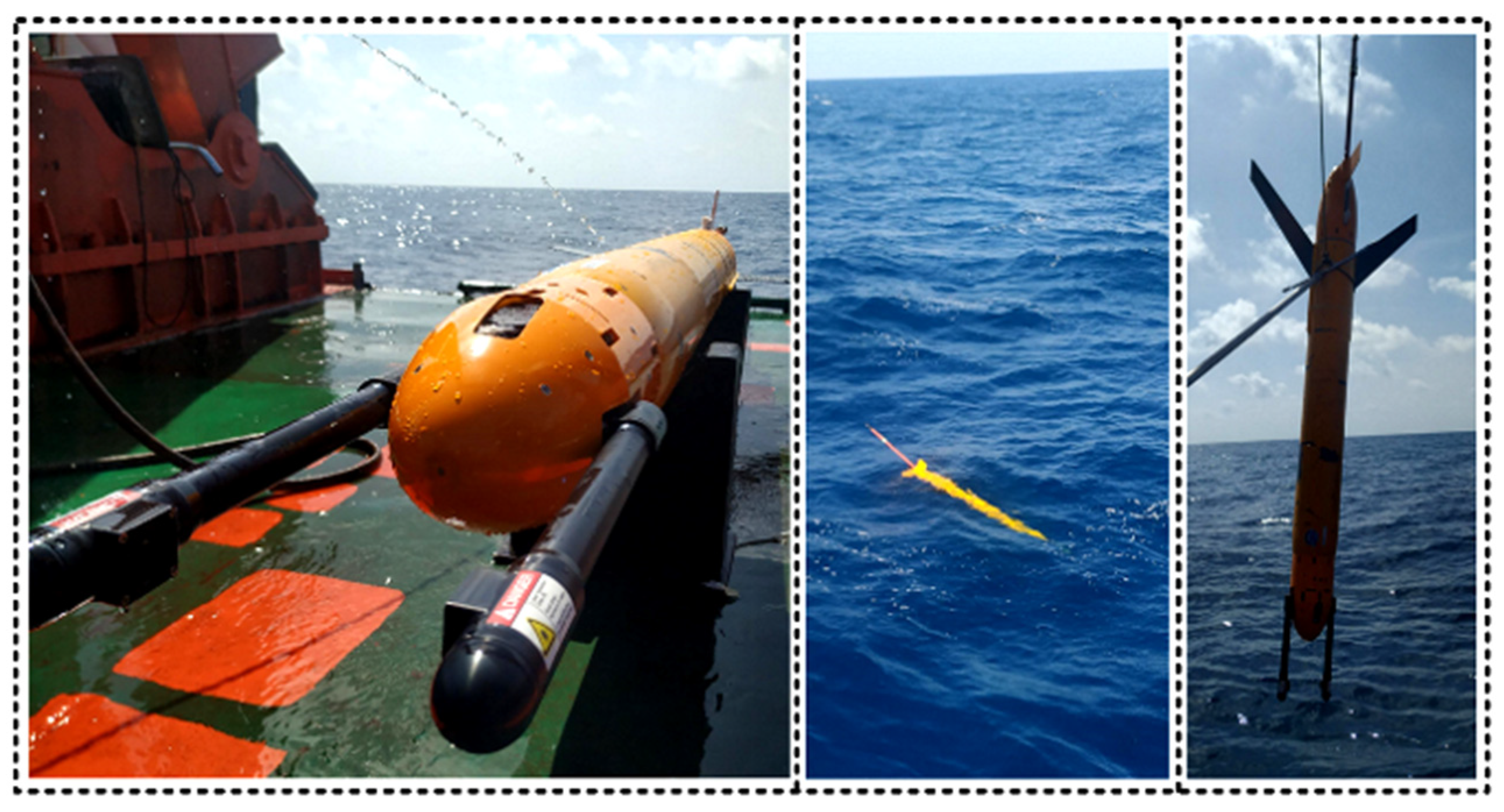
The DHUG, as shown in Figure 1, is an integrated design using the hybrid-driven “Petrel-II” glider from China [31], which is equipped with an in-line, lens-free digital holographic system produced by Seascan Inc. (Falmouth, MA, USA) (Figure 2) for observing marine plankton in the size range of 1–10 mm. Compared with traditional underwater gliders, the “Petrel-II” is equipped with a small propeller at its tail, greatly improving its maneuverability underwater and allowing it to cruise at a fixed depth. The “Petrel-II” glider adjusts its attitude by rotating and moving its internal battery package. It navigates using GPS, and the control commands and data between the shore-based control center and glider are transmitted by Iridium satellites. For other parameters, refer to the literature [32]. The “Petrel-II” has proven to have an excellent performance in extensive sea trials. The DHUG is capable of three working patterns: a sawtooth glide for horizontal and vertical sampling, a spiral glide for critical areas, and a fixed-depth cruise for a particular water zone. Hence, these three patterns can be flexibly combined to realize in situ marine plankton observation according to the operating conditions.

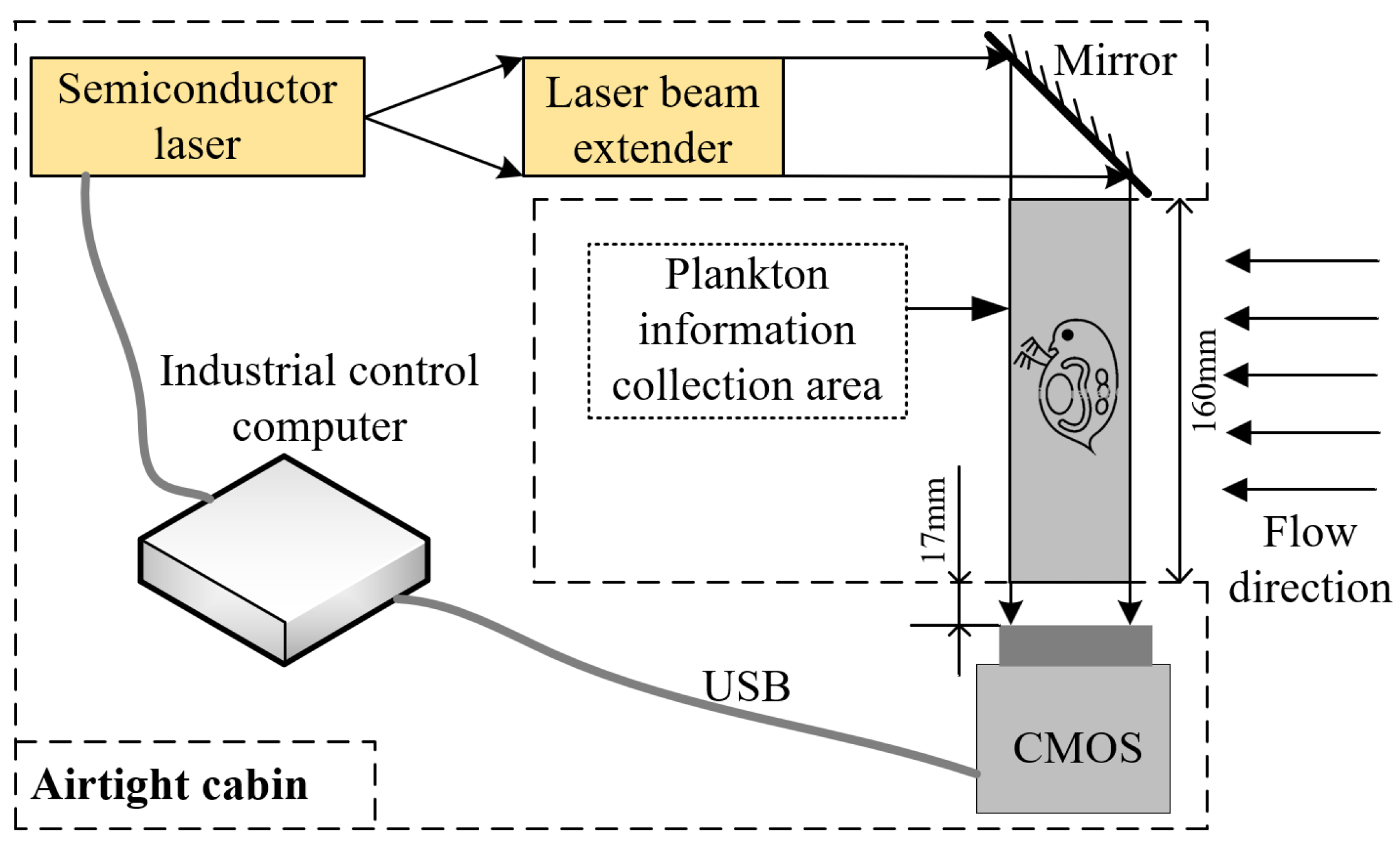
The DHUG’s in-line, lens-free digital holographic system integrated on the glider has a simple optical path, and the space it occupies is further compressed by folding the laser propagation path with a prism. It is suitable to install the device on a small underwater vehicle, given its low power (operating at a maximum power consumption of 6.4 Wh) and relatively larger sampling volume per burst (particle size distribution and concentration size range of ~25–2500 μm and sampling volume per hologram of 20.3 mL). The holographic imaging system is integrated in front of the glider to avoid interference with plankton caused by ambient turbulence when the glider is moving.

In the system, when a coherent beam emitted by the laser (wavelength λ = 658 nm) passes through the beam expander and a high-quality collimated plane wave is obtained, which is reflected by the mirror. The particles in the water scatter part of the target beam, and the remaining undisturbed reference beam interferes with the scattered one to form a holographic image, which is then captured by a complementary metal-oxide-semiconductor (CMOS) camera placed at the end of the light propagation. The holographic imaging system uses CMV4000 USB3 mono industrial camera (ams-OSRAM AG, Premstaetten, Styria, Austria) (specification: 11.27 mm × 11.27 mm, 2048 × 2048, 5.5 μm × 5.5 μm pixels, 90 fps refresh rate) that can be set to capture holographic images (approximately 4.09 MB in size) at a frequency of 1–10 Hz. These holographic images captured by the camera are transferred to the single board computer via the camera adapter board and stored on a 2 TB hard disk, which can operate for 13.5 h at 10 Hz. The operating commands by the holographic imaging system are simultaneously sent to the internal control computer of the “Petrel-II” glider. In addition, a GPCTD is mounted on the tail of the glider to obtain the thermohaline structures of the in situ sampling at a frequency of 1 Hz. Once the sampling task is completed, the holograms stored on the hard disk are downloaded onto a PC to extract the suspended particle images and estimate the plankton size and abundance, a process which is described hereinafter in more detail.

2.2. Observation

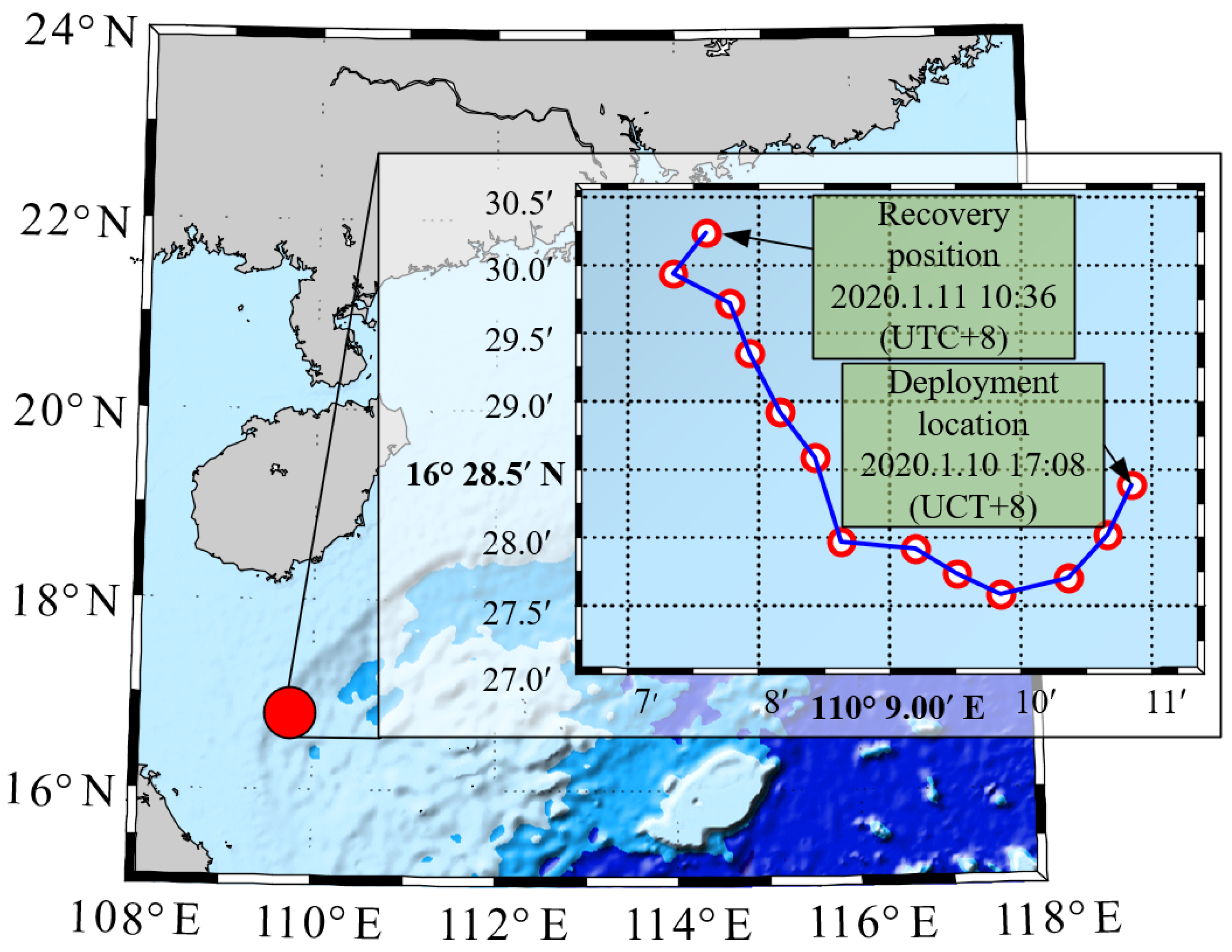
The DHUG began its observation on 10 January 2020 along a planned course near the continental slope in the South China Sea. After testing its various functions, the DHUG was deployed into the designated sea area (16°27.70′ N, 110°10.37′ E), and it moved in a sawtooth gliding pattern with a pitch angle of approximately 28° and a maximum diving depth of 600 m. The trajectory of the DHUG is shown in Figure 3.

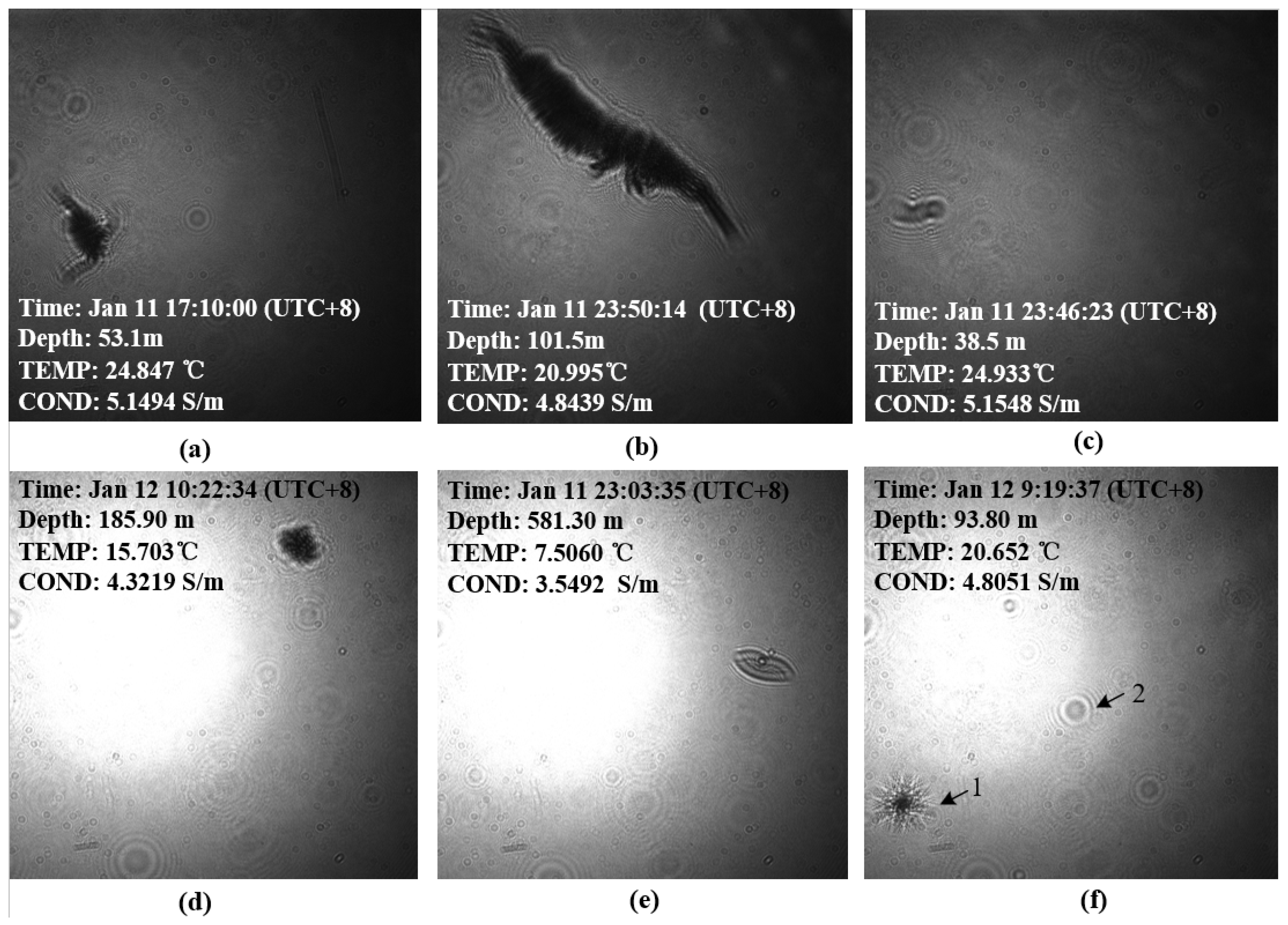
During this mission, the steady gliding velocity of the DHUG was approximately 0.8 m/s, and the holographic camera’s frame rate was defined at a 4-Hz frequency, namely, that 20.3 mL of seawater was sampled at every vertical interval of nearly 5.2 cm. The DHUG obtained data from 11 profiles, obtaining 11 segments of holographic images and the corresponding hydrological information, including temperature and conductivity. A total of 206,059 holograms were obtained, meaning that 4183 L of seawater samples were collected. Figure 4 shows random and classic holographic samples taken at different times. This paper will set out the process of the image processing using the holographic samples.

3. Methods for the Investigation of Marine Plankton

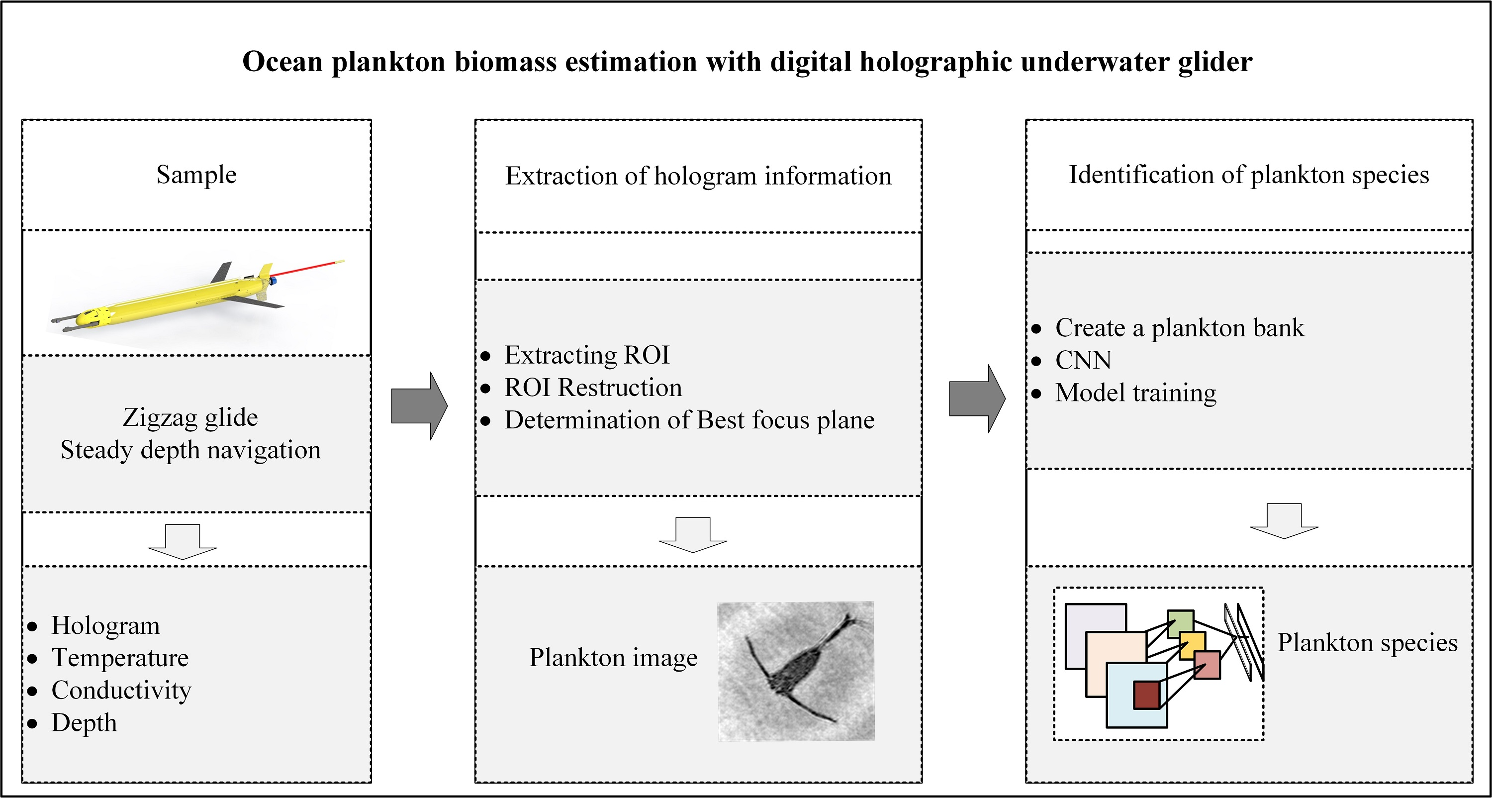
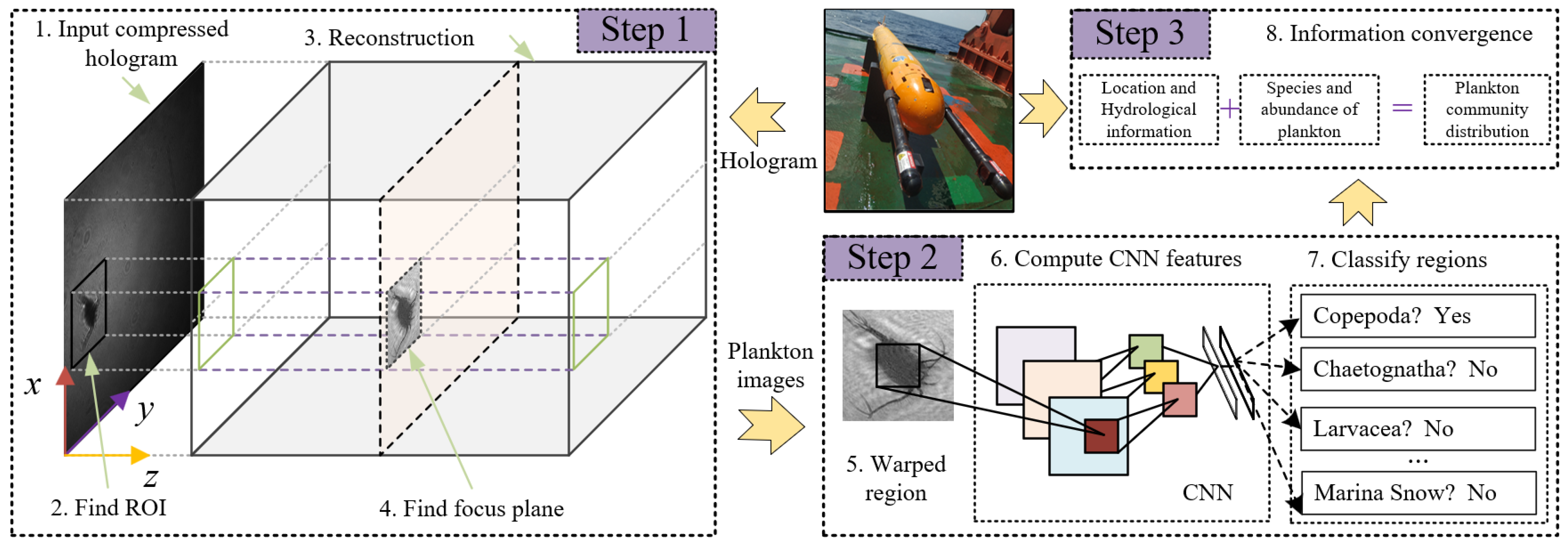
To automatically access the spatio-temporal distribution of plankton from the hologram images taken by the DHUG, three successive steps are undertaken, as shown in Figure 5. Step 1 is to extract the plankton images from the hologram. First, the position of the plankton in the holographic image (the x, y coordinates) is determined by background subtraction. The hologram is compressed to accelerate the data processing, and this step enables a rough estimation of the suspended particle concentration. Then, the extracted plankton region is reconstructed using the angular spectrum method (ASM), and the Sobel variance (SOL_VAR) focusing algorithm improved in this study is adopted to determine the axial position of the plankton in the hologram (the z coordinates). Step 2 identifies the extracted plankton species. The extracted plankton images are imported into the convolutional neural networks (CNN) to identify the plankton species. Step 3 depicts the relationship among the plankton information, the location of the DHUG, and the collected thermohaline structure.

3.1. Extraction of the Hologram Information

This section details a fast and automatic method for extracting suspended particle images from a sequence of holographic images taken by the DHUG and determining the size of the suspended particles. The basic process includes identifying the region of interest in the holographic image, reconstructing the region of interest, and, finally, finding the focus plane. This method focuses solely on the holographic images with the suspended particle, and it significantly enhances the holographic image processing efficiency by sacrificing image resolution (somewhat) in practice.

3.1.1. Extraction of the ROI from the Holograms

As shown in Figure 2, the collimated plane light is formed after the laser source passes through the laser beam expander, and the maximum intensity is found at its center. The intensity gradually decreases in a radially outward direction and follows a two-dimensional Gaussian distribution. The laser power is suppressed to reduce the power consumption of the holographic imaging system, which accounts for the uneven intensity of the hologram taken by the DHPG, as shown in Figure 4. This phenomenon also exists in the images captured by the 4-Deep HoloSea digital inline holographic microscope (DIHM) [11].

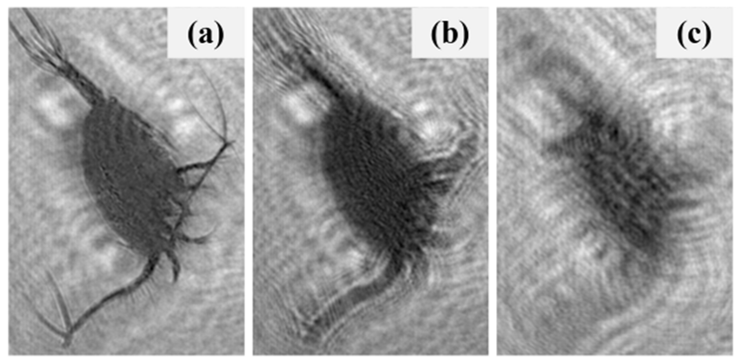
The DHUG experiences considerable changes in ambient light intensity and temperature when performing sawtooth profiles, dramatically affecting the laser output power and holographic image quality. The power of the laser decreases as the ambient temperature increases. As shown in Figure 4a–c, the high ambient temperature and dark light lead to a very low hologram intensity. On the contrary, despite the weak ambient light at 518 m shown in Figure 4e, the increasing laser emission power caused by the low temperature improves the intensity of the holographic image. Using a function of threshold or adaptive threshold to extract the region of interest (ROI) in this case does not yield good results, and it may lead to a low probability in the detection or even ignorance of the edge part of the particles. For this reason, a method based on a probabilistic ROI detection that is irrelevant to the intensity size and distribution of the holographic image is presented to improve the efficiency of particle recognition. In processing the hologram images acquired by the DHUG, the uneven laser beam intensity and the inherent system noise on the holographic camera lens are backgrounds. The variations of hologram intensity due to the changes of ambient light and laser output power are regarded as the variation of ambient light intensity, and the hologram intensity varies evenly with the depth. Dealing with time-series holograms of inhomogeneous and variable intensities is then converted into detecting moving targets against a static background. The position of the plankton in the hologram image is determined using the background subtraction method. Subtracting the hologram from the reference image obtains a differential image, which is then binarized to obtain the plankton position. The key to acquiring an appropriate ROI by background subtraction lies in constructing a robust reference image to weaken or even eliminate the light intensity variation of the holograms. Here, a classical adaptive hybrid Gaussian background modeling method for holograms is adopted [33]. The following is a brief description of the approach.

Suppose that each pixel of a series of holograms taken continuously consists of k Gaussian distributions. Then, the probability density function of a pixel at time t can be expressed as:

$$P\left(X_t\right)={\displaystyle \sum _{i=1}^{\mathrm{K}}{\omega }_i}\eta \left(X_t,{\mu }_i,{\Sigma }_i\right)$$

(1)

where ω is the weight of the kth Gaussian distribution, $\eta \left(X_t,{\mu }_i,{\Sigma }_i\right)$ is the probability density function of the kth Gaussian distribution, ${\mu }_{\mathrm{i}}$ is the mean value of the kth Gaussian distribution, ${\Sigma }_i={\sigma }_k^{2}I$ is the covariance matrix for the kth Gaussian distribution, ${\sigma }_k^2$ is the variance, and I is the unit matrix. By arranging the k Gaussian distributions in the order of magnitude of the ${\omega }_k/{\sigma }_k$ value, the background model can be estimated as follows:

$$B=\arg \min \left({\displaystyle \sum _{i=1}^b{\omega }_i}>T\right)$$

(2)

where the threshold T is the minimum fraction of the background model. The binary image is obtained by matching the hologram, $I\left(x,y\right)$, to the background model, and then the position of the ROI in the holographic image is extracted by performing opening and closing operations on the image to remove the noise. The background model is updated in real-time by the Oline EM algorithm, wihch is detailed in [33].

Before modeling the hologram sequences with a hybrid Gaussian background, the holograms need to be scaled down to the same scale and filtered with a mean filter to enhance the processing speed and accuracy of the background modeling. Influenced by the diffraction halo, a single plankton may be mistaken for multiple planktons. This phenomenon is overcome by merging the overlapping parts of the ROIs. The above procedure reduces the possibility of large particles being partitioned at lower suspended particle concentrations. However, it is possible to underestimate the particle concentration when the concentration of suspended particles is extra high.

3.1.2. ROI Reconstruction

In digital holography, a holographic image is reconstructed by simulating the spatial propagation of light with numerical calculations to recover the distribution of the object wave on the original plane based on the diffractive plane in which the hologram is located. Commonly, the methods for reconstructing holograms include the Fresnel diffraction method (FDM) and angular spectrum method (ASM). The ASM differs from the FDM in that the reconstructed image pixels are the same size as the holographic image pixels, and they are independent of the reconstruction distance [34,35]. It is more suitable for application in in-line holography to analyze the distribution of particles dispersed in transparent media [35]. Further, unlike the 4-Deep HoloSea [11], the in-line holographic imaging system applied in the DHUG is lens-free and the photographed holograms are not scaled, and so the resolution of the reconstructed image using ASM is equal to that of the camera. This advantage makes it easier to extract the shape features of the plankton. The ASM reconstructs the ROI, which can be represented as:

$$\psi (x,y,z)={\mathcal{F}}^{-1}\left\{\mathcal{F}\right\{I(x,y)\}\times \mathcal{H}(x,y;z)\}$$

(3)

where $\mathcal{F}$ is the Fourier transform, ${\mathcal{F}}^{-1}$ is the inverse Fourier transformation, $I(x,y)$ represents the light intensity distribution of the holographic image, and $\mathcal{H}(x,y;z)$ is the space–frequency transfer function after the wave propagation distance z. The space–frequency transfer function in the near-axis approximation can be expressed as follows:

$$\mathcal{H}(x,y;z)=\exp \left\{\frac{i{k}_{0}z}{2}\left[{\left(\frac{{\lambda }^{\prime }x}{k_0}\right)}^2+{\left(\frac{{\lambda }^{\prime }y}{k_0}\right)}^2\right]\right\}$$

(4)

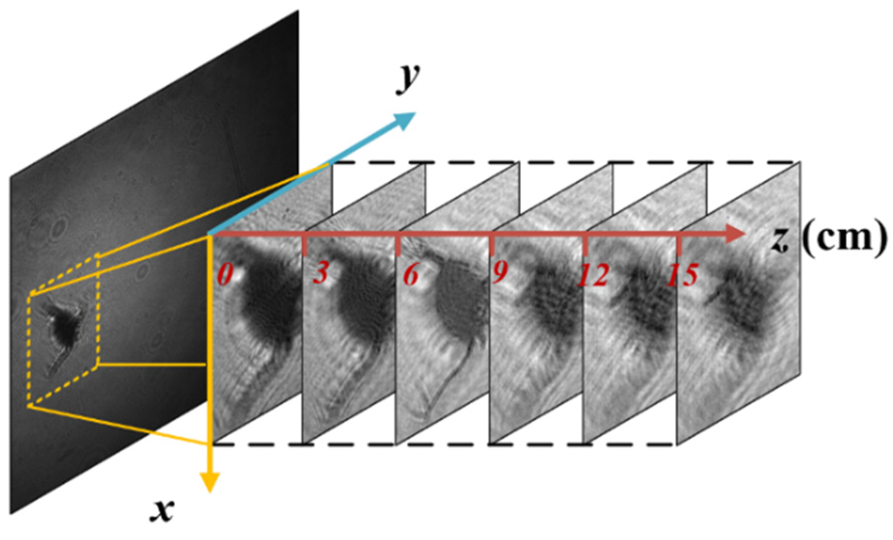
where $k_0=\frac{2\pi }{{\lambda }^{\prime }}$, z represents the distance to the hologram plane, ${\lambda }^{\prime }=\frac{n_a}{n_w}\lambda$ is the wavelength at which the laser propagates in the medium, and $n_a$ and $n_w$ are the refractive indexes of the laser in the air and seawater, respectively. By adjusting z in Equations (3) and (4), any of the cross-sectional images in the imaging volume can be obtained. Figure 6 shows the reconstructed image using ASM in the sampling volume.

Since the zero-order diffraction in the hologram affects the quality of the reconstructed image, it should be removed before reconstructing the hologram. Schnars and Jüptner [36] proposed a method to remove such interference in reconstructed images by subtracting the average intensity from the holographic images [36]. It can be expressed as:

$$I^{\prime }(x,y)=I(x,y)-\frac{1}{MN}{\displaystyle \sum _{x=0}^{M-1}{\displaystyle \sum _{y=0}^{N-1}I}}(x,y)$$

(5)

where $x=0,\dots ,M-1;y=0,\dots ,N-1$; and M and N represent the number of pixels, along with the directions of x and y, in the reconstructed image, respectively. Alternatively, high-pass filtering can also replace it with a low cutoff frequency [36].

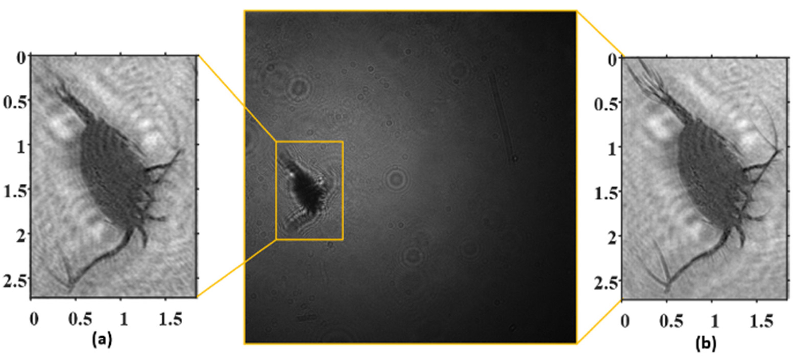
There may be only single plankton, or even nothing, in a holographic image taken in the South China Sea, as shown in Figure 4. Therefore, the reconstruction procedure is inefficient if all the holograms are selected. Hence, only those ROIs where plankton information is presented are reconstructed. The two Copepoda images shown in Figure 7 are the result of reconstructing a partial holographic image and the whole holographic image in Figure 4a, respectively. It can be seen that although the image quality is degraded, the processing time is greatly reduced. Therefore, for extracting plankton information from millions of holographic images that contain few plankton, it is worthwhile and necessary to sacrifice a small amount of image quality for processing efficiency. In addition, if a high resolution is required, the size of reconstructed images can be augmented appropriately.

3.1.3. Determination of the Best Focus Plane

The reconstruction of the ROI in the holographic images can obtain arbitrary cross-sectional images in the sampling volume, as shown in Figure 6. The in-focus and out-of-focus phenomena exist in those reconstructed images. Finding the best focus plane is the final and critical procedure in holographic information extraction, and it is directly related to the quality of the plankton images obtained by the holographic imaging system and to the accuracy of the plankton recognition. Many algorithms have been proposed for tackling the problem, such as the Wavelets, Laplacian (LAP), Tenengrad (TENG), Area Metric, and Maximum Total Intensity (MTI) [30,37,38]. Dyomin and Kamenev [39] extracted plankton images from holographic images using the TENG algorithm. Davies et al. [19] applied a simple and fast MTI function to locate the axial position of suspended particles and embedded this algorithm into the accompanying software in Sequoia’s LISST-Holo.

The Sobel variance (SOL_VAR) algorithm is adopted in this work to find the best focus plane in reconstructing holographic images. This algorithm, proposed by Pech-Pacheco, Jose Luis, and Cristobal [40] in their study on high-powered microscope focusing algorithms, presents a better robustness to noise than the TENG algorithm, and it maintains a good performance, allowing for appropriate changes in the focus window and the presence of noise.

The SOL_VAR algorithm is expressed as:

$$Z_{\mathrm{focus} }=\arg \underset{z}{\max }\sigma \left\{\begin{array}{l}{\left[ROI(x,y,z)\otimes S_x\right]}^2\\ +{\left[ROI(x,y,z)\otimes S_y\right]}^2\end{array}\right\}$$

(6)

where $S_x$ and $S_y$ represent the Sobel operator convolution kernels in the x- and y- directions, $\left(\begin{array}{ccc}-1& 0& 1\\ -2& 0& 2\\ -1& 0& 1\end{array}\right)$ $\left(\begin{array}{ccc}1& 2& 1\\ 0& 0& 0\\ -1& -2& -1\end{array}\right)$, respectively; z is the reconstruction distance ($z_{down}\le z\le z_{up}$); σ represents the variance of the matrix; and $ROI\left(x,y,z\right)$ represents the reconstruction of the ROI in the holographic image at the distance z.

The algorithm is compared with TENG and MTI.

The TENG algorithm is expressed as:

$$Z_{\mathrm{focus}}=\arg \underset{z}{\max }{\displaystyle \sum _{x=0}^{M-1}{\displaystyle \sum _{y=0}^{N-1}\left\{\begin{array}{l}\left[ROI(x,y,z)\otimes S_x\right]\\ +\left[ROI(x,y,z)\otimes S_y\right]\end{array}\right\}}}$$

(7)

The difference between SOL_VAR and TENG is that after calculating the gradient of the image by the Sobel operator, the former performs the variance calculation while the latter performs the summation operation.

The MTI algorithm can be expressed as:

$$Z_{\mathrm{focus}}=arg\underset{z}{max}\sum _{x=0}^{M-1}\sum _{y=0}^{N-1}\left[ROI(x,y,z)\right].$$

(8)

Finally, the images of each plane shown in Figure 6 (the reconstruction step is set to be 5 mm) are calculated and normalized according to the three algorithms to assess the effects (Figure 8). The locations of the best focus planes obtained by the three methods are listed separately in Figure 9. It can be seen that SOL_VAR obtains the best focus position, while the image obtained by the TENG algorithm deviates from the actual position, and MTI has a peak at the best location, but the result is masked by noise. The SOL_VAR algorithm outperforms two other methods in terms of unbiasedness, single-peak, and sensitivity to noise. The strengths and weaknesses of this algorithm will be explored in more detail.

3.2. Identification of Plankton Species

The number of plankton images extracted from holograph sequences can be immense in volume. Estimating plankton abundance manually is laborious and time-consuming. Therefore, it is necessary to boost efficiency for identifying the extracted planktonic images with an automatic algorithm. The traditional classification of suspended particle images by feature extraction has been developed, to some extent [19,29,41]. However, with the increasing number of suspended particle species, the feature extraction method cannot be adapted to the classification task with a wider variety of plankton species. With the continuous development of deep learning, a convolutional neural network (CNN) has proven extremely efficient for learning and classifying features from end to end. A CNN consists of the main input layer, a convolutional layer, a pooling layer, a fully connected layer, and an output layer, and ResNet-50, with its high accuracy and fast speed characteristics, is involved in classifying the extracted plankton images. It uses the residual network to allow a deeper, faster convergence and easier optimization of the network while having fewer parameters and less complexity than previous models, and it addresses the problem of degraded, hard-to-train networks [42]. The trained ResNet-50 network is added to the CNN of Figure 5 to complete the identification of plankton species in the hologram.

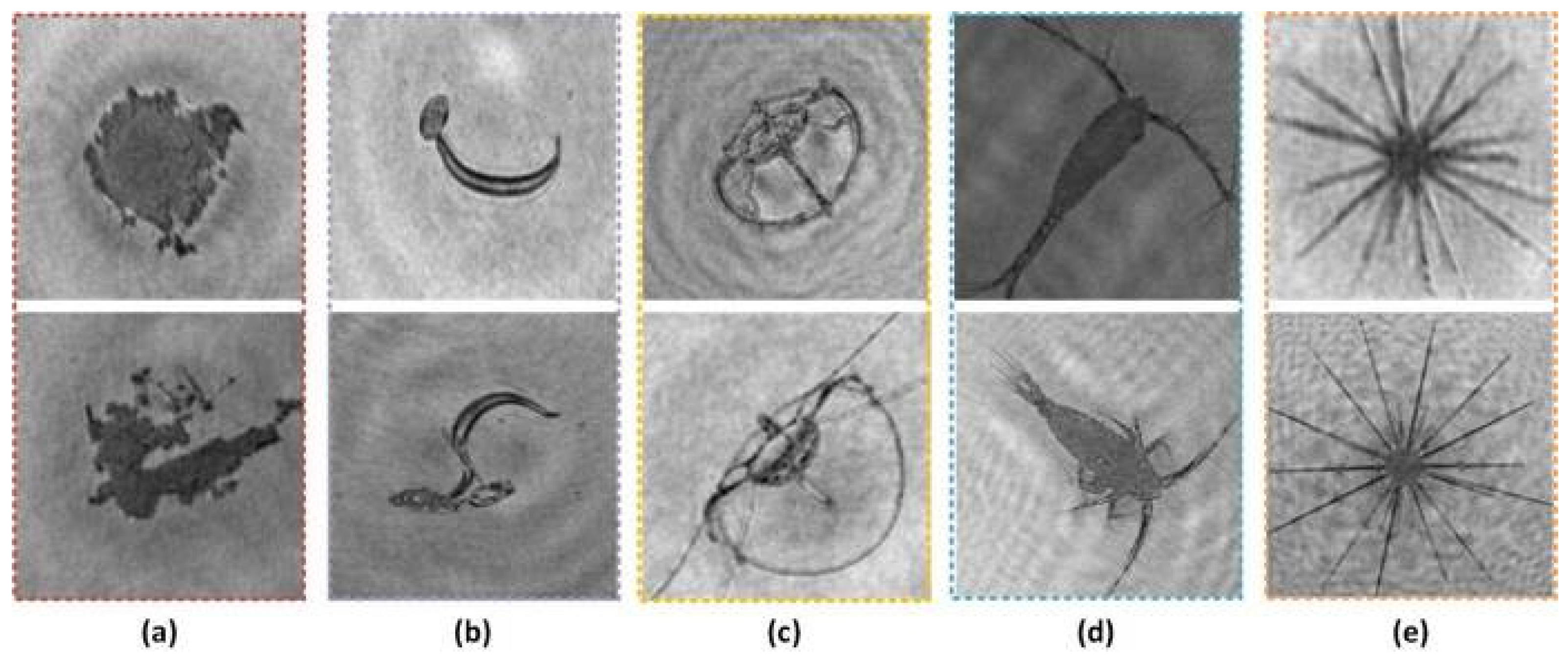
For training, the CNN, ResNet-50, which is pre-trained with millions of images in Image-Net, is regarded as the starting point of the network. The feature extraction layer of this network is retained, replacing the output layer with the plankton species. The parameters of the feature extraction layer are fixed, and only the parameters of the fully connected layer are trained. Given the number of plankton databases, we randomly selected 50% of samples as a training set, 20% as a validation set, and the remaining 30% as a test set. In the process of building the database, several common types of zooplankton and suspended particles (the Copepoda, Marina snow, Oikopleura, Medusa, and Acantharian species shown in Figure 10) in the experiment are taken for training the CNN. To compensate for the out-of-focus particles, since the actual focus plane of the particles is not reconstructed, the image of the particles with the best focus plane and the two images adjacent to the focus plane are selected in this procedure. Further, the operations of zooming, rotation, translation, and mirroring of the particle images in the database are performed. The aims of these operations is to expand the number of images in the training set and reduce the overfitting of the neural network.

4. Assessment and Discussion

In order to evaluate the feasibility of marine plankton observation using the DHUG, this section discusses the algorithm proposed in this paper in terms of the use of DHUG in the estimation of ocean-suspended particle concentration, plankton images extraction, and plankton abundance statistics. The algorithm is written in Matlab2017 (MathWorks, Natick, MA, USA) and runs on a mobile workstation with an Intel Core i5-8400H CPU 2.5 Hz with 32 GB of RAM.

4.1. Estimation of Suspended Particle Concentration

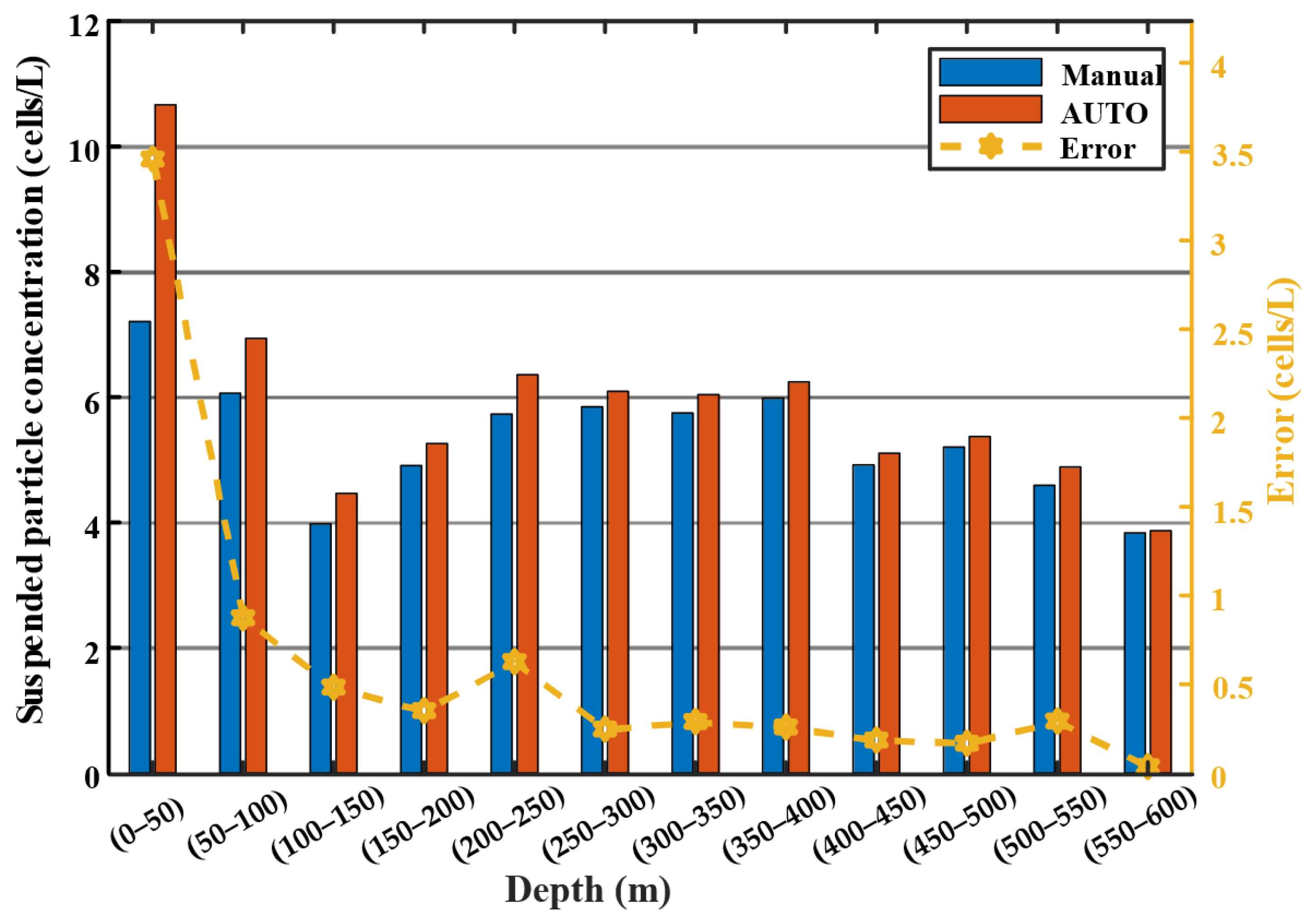
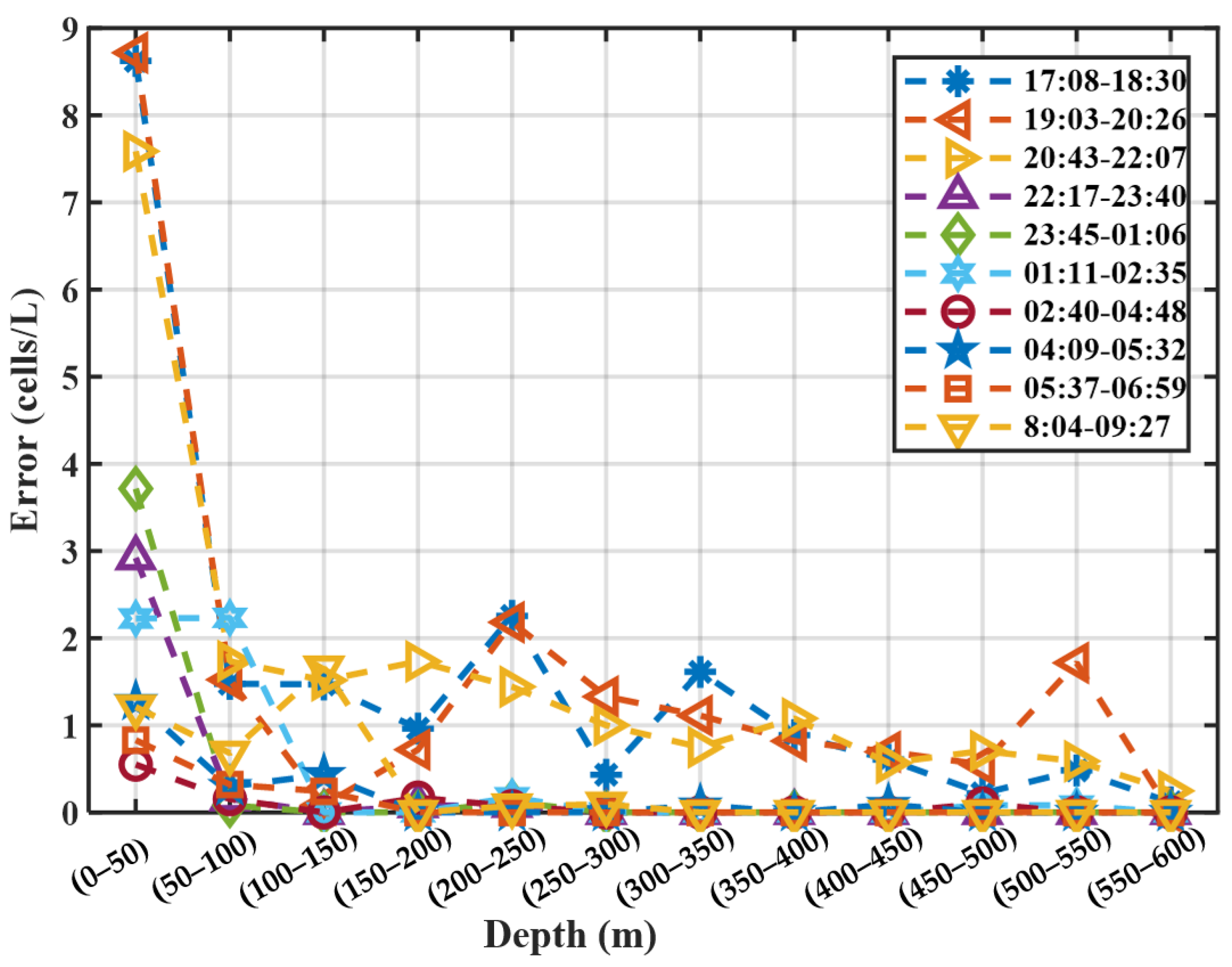
The sampling image volume of the digital holographic system is fixed, and so the concentrations of the suspended particles can be estimated by counting the number of ROIs in each holographic image. To further speed up the processing of hologram sequences and to ensure processing accuracy, the scaled holograms are conservatively scaled from 2048 × 2048 pixels to 480 × 480 pixels. Figure 11 illustrates the concentrations of the suspended particles obtained automatically (blue) and manually (red) at different depths, summarized from all the data collected by the DHUG in the South China Sea. Manual processing may affect the statistical results due to operator fatigue, etc., but the manual processing results are assumed to be accurate. The error represents the difference between the suspended particle concentrations obtained by automatic and manual treatment. The relationship between the suspended particle concentration error and the depth is obtained by the automatic processing of the hologram sequences taken by the DHUG at different profiles, as shown in Figure 12.

According to the previous assumption, the statistical results show a high similarity between the results obtained from automatic extraction and those from manual processing, but the automatic processing overestimates the particle concentrations and the error between the two approaches tends to decrease with depth. The automatic processing results of a holographic image acquired from below 50 m at different profiles are pretty good, but they contain larger errors in the shallow water. In general, the number of suspended particles in the holographic image obtained by subtracting the background is accurate. Figure 11 shows that the error between the automatic and manual analysis is less than 0.9 cells/L when the depth is greater than 50 m, and it decreases with increasing depth. According to Figure 12, this is even true for all holographic images taken at different times. A maximum error exists at above 50 m, and this value is highly related to the sampling time.

The refractive index is uneven in different areas of seawater. When light enters seawater, it forms filamentary strips of light, affecting the holograms captured by the holographic camera, and resulting in a large gap in the intensity distribution of the images. This phenomenon may lead to algorithm failure during the detection of the ROI. Taking the filamentary light bar as an ROI can lead to an overestimation of the particle concentrations, but this disturbance progressively diminishes as the depth increases. Therefore, the automatic suspended particle concentration error analysis decreases gradually with increasing depth. In addition, the hologram intensity is affected by the laser intensity and ambient light, and so the environmental noise greatly influences the hologram with relatively low intensity. The automatic extraction of the ROI algorithm can perform well in the case of high hologram intensity. A low-light holographic image results in protruding filamentous light bars, and thus an overestimation of the particle concentrations. This phenomenon is contrary to Walcutt et al. [11], who mentioned that the particle concentrations would be estimated in low-light regions at the boundaries of the holograms.

Although the size and morphological parameters of a suspended particle cannot be determined in this section, an estimation of concentration can be quickly performed based on millions of collected holographic images. This method is less effective in dealing with the data collected by the DHUG at depths of less than 50 m, but it will further improve the accuracy in estimating suspended particle concentration by improving the performance of the laser system to reduce the sensitivity to temperature, which is also a direction of effort in the future. The statistical results show that nearly 75% of the holographic images present no suspended particles, which verifies that it is necessary to first confirm the existence of the ROIs in the images to shorten the processing time of the holograms.

4.2. Plankton Image Extraction

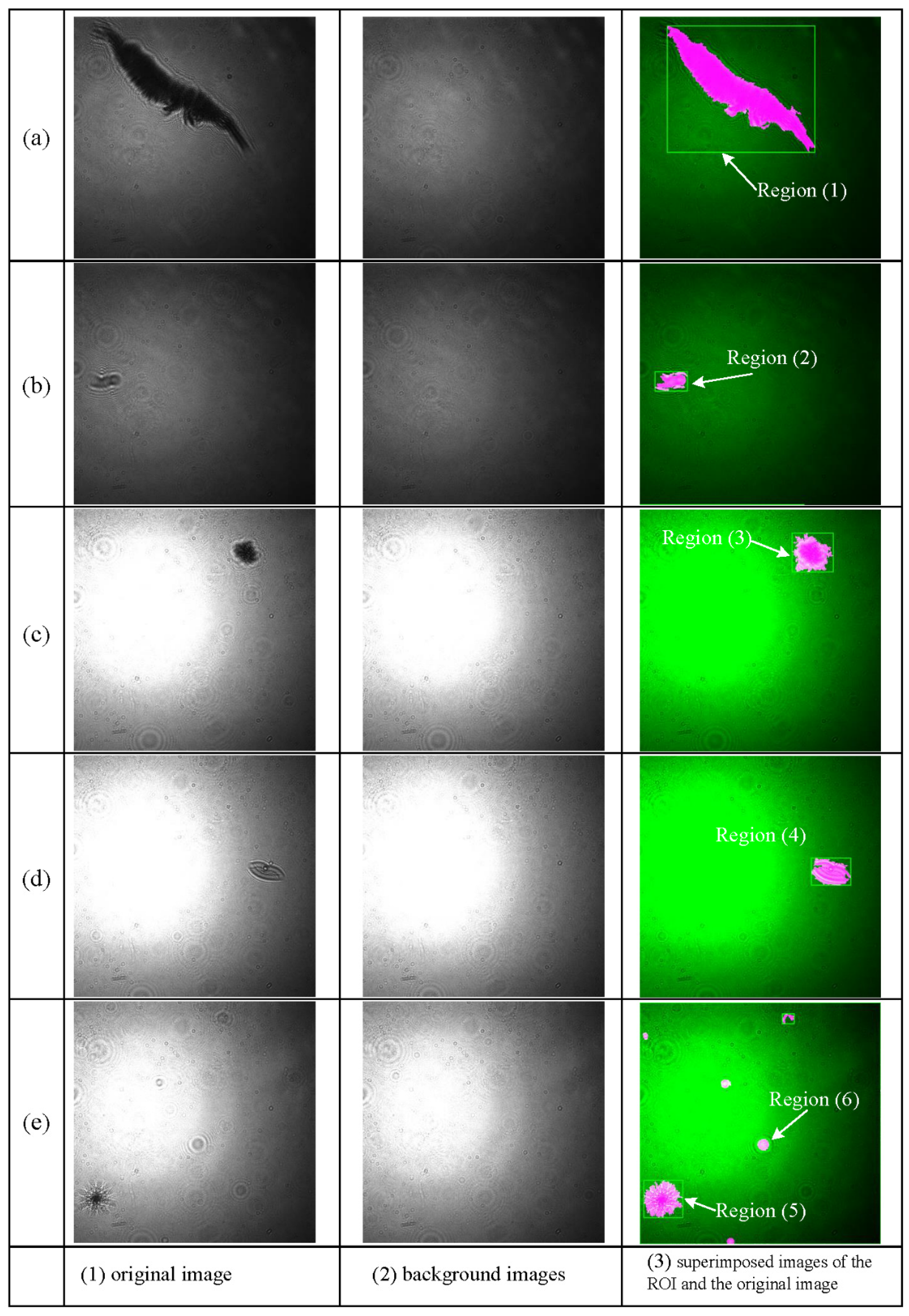
Some of the most common plankton species in the ocean are selected to evaluate the quality of the extracted information from the holographic images. The extraction of an ROI in the holographic image and autofocusing are demonstrated in this section. Figure 13 presents the location of an ROI obtained by background subtraction. The left column shows the original holographic images. The middle column shows the corresponding background images. The right column shows the effect of superimposing the original holographic images, the binarized images, and the minimum boundary box of the suspended particles. The holograms are reconstructed with a step size of 5 mm for the ROIs, and 33 plane images between the sapphire windows are obtained. 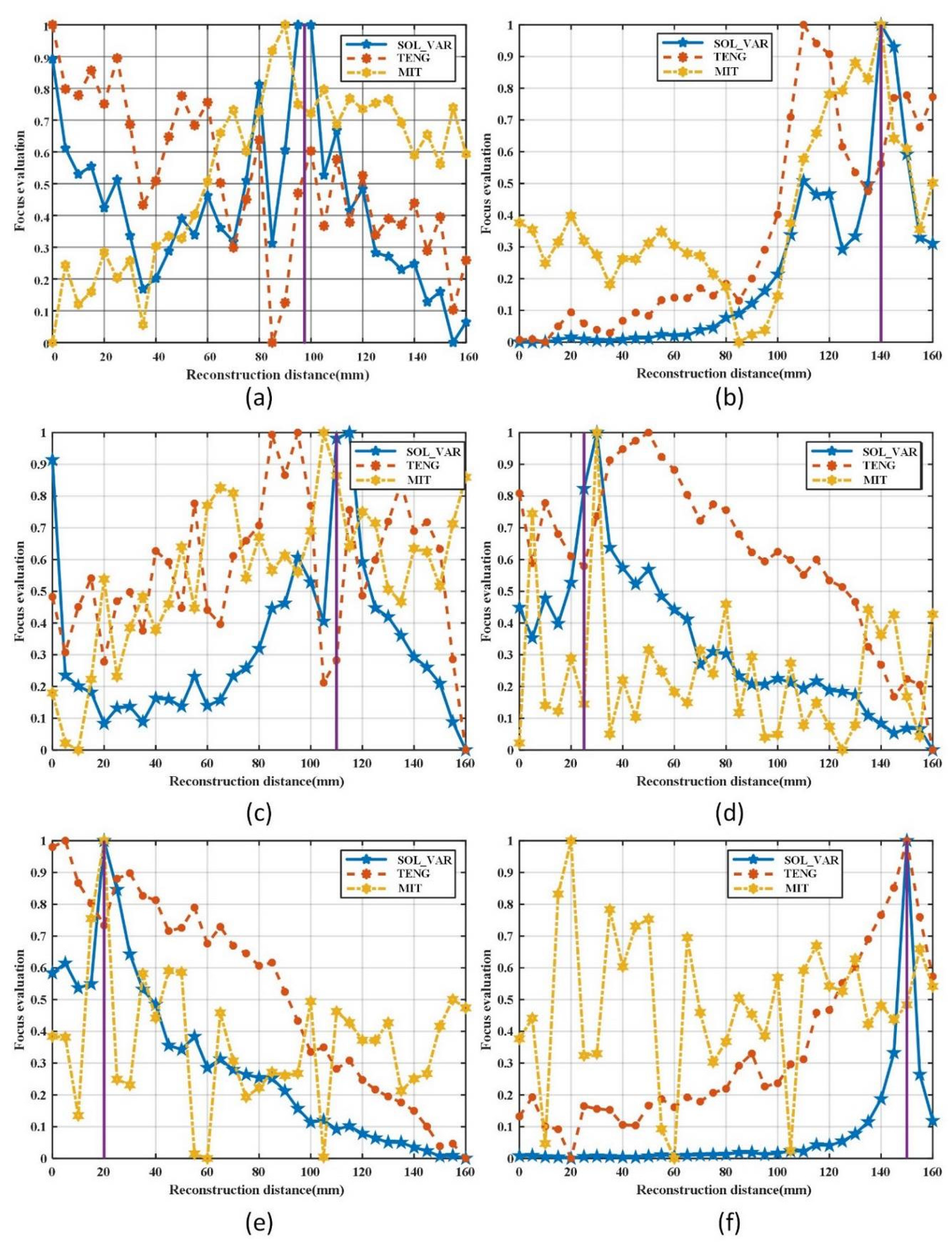Figure 14 is obtained through the focus evaluation function for each plane image. Figure 14a–f corresponds to regions 1–6 in Figure 13, respectively, and the purple vertical lines represent the positions of the manually selected focus planes. 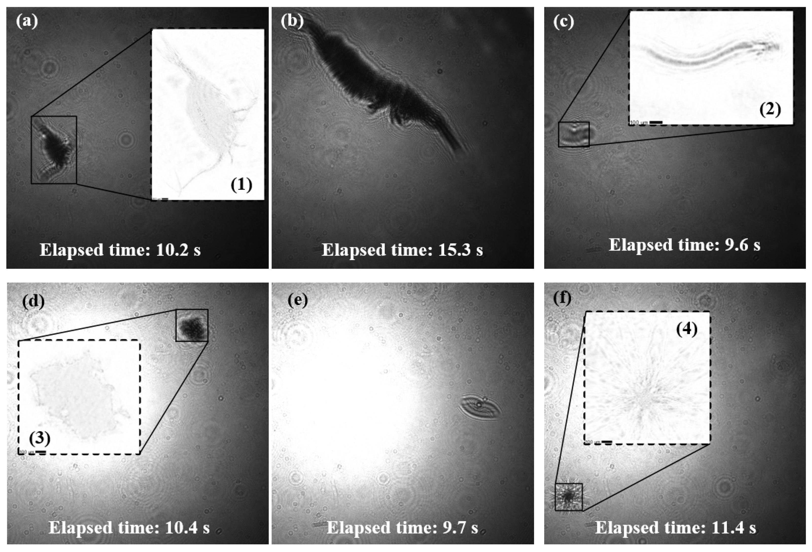Figure 15 shows an image of the plankton on the focus plane automatically obtained using the SOL_VAR method.

The intensity variation of the holograms in Figure 13a–e can accurately locate the positions of the suspended particles in the hologram images. Since the diffraction spots formed by the suspended particles in the hologram are larger, the minimum boundary box in regions 2–6 defined in Figure 13 is larger than the plankton volume for better light transmittance. The 1.5 mm suspended particles at the edge of the hologram in Figure 13e are well detected when the hologram intensity distribution is not uniform. The choice of thresholds in adaptive hybrid Gaussian models and the updated model speed is directly related to the quality of the detection results. Further, the morphological calculations on the graph affect the splitting of the suspended particles into multiple particles. Appropriate parameters are applied in the automatic calculation by adjusting the model, and the test results on typical plankton are satisfactory. However, the fragmentation issue of plankton with very long tentacles still exists.

The auto-extracted ROI whose area is greater than that of plankton places higher demands on the focus algorithm. Figure 14, obtained by evaluating the focus positions of regions 1–6 in Figure 13, shows that the location of the best focus plane determined by SOL_VAR is basically identical with the manual processing results. The SOL_VAR function outperforms the MTI and TENG algorithms in terms of unbiasedness, single-peak, and generality. Due to noise, the TENG algorithm is only accurate for region 6 in the focus plane of Figure 13. The MTI algorithm runs faster than other algorithms, but with lower accuracy than SOL_VAR. These three algorithms obtain multiple local peaks, as shown in Figure 14. This phenomenon may be due to the noise in the water and the fact that the plankton are stereoscopic. Figure 14a,c obtains a high score in the initial plane of the reconstruction, where it there locates the sapphire window with stationary objects. In Figure 14a,c,d, the focus plane positions obtained by SOL_VAR deviate from the actual ones (denoted by the purple lines), which is caused by the fact that the best focus plane is not reconstructed. To obtain a more accurate focus plane position, the solution is to reduce the reconstruction step size. However, such a method is not recommended as it will greatly increase the processing time.

The plankton images extracted from the holograms in Figure 15 demonstrate the feasibility of the fast method proposed in this study for extracting hologram information. The tentacles are well preserved for the plankton ranging in size from 0.2 mm (Copepoda) to 9 mm (krill). Under a low concentration of suspended particles, locating the position of the plankton in the holographic image before extracting its information will greatly minimize the information extraction time. At least 75 percent of the time has been saved in processing the data collected in the South China Sea. Figure 16 shows the montages obtained with Holo-Batch processing algorithm accompanying the LISST-Holo system [19,30]. The algorithm used in this software runs well for observing bubbles and diatoms, but it is ineffective for plankton extraction. The results show that the new algorithm proposed in this study significantly improves the quality of the extracted images, reduces the over-segmentation of macro-plankton, and significantly shortens the processing time compared to the Holo-Batch algorithm.

4.3. Spatio-Temporal Distribution of Marine Plankton

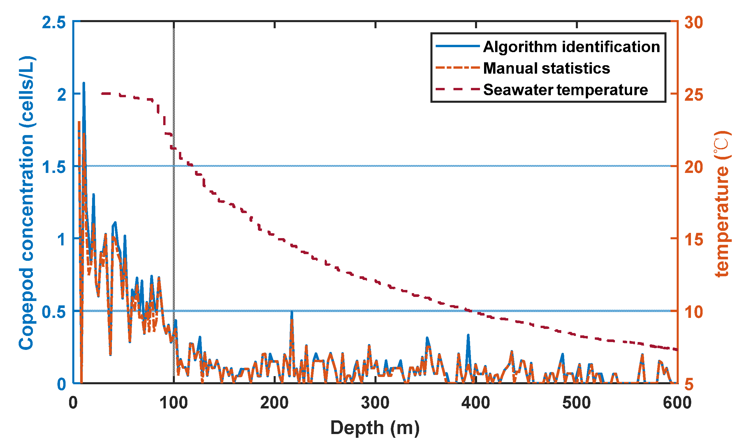
By training the CNN with the established plankton library, a validation accuracy of 88.36% is finally obtained, and the automatically extracted plankton images are imported into the CNN for plankton species identification. Furthermore, the spatio-temporal distribution of the plankton is obtained by combining the hydrological information collected by the DHUG. The most common Copepoda in the ocean is taken as an example here. The object detection method for holographic images is applied for processing the holographic sequences taken in this sea trial to obtain the relationship between the number of Copepoda and the depth, as shown in Figure 17.

The statistical results show that the biomass of plankton obtained through automatic estimation and manual processing at different depths show the same tendency, despite the certain error between these two. In the future, we will continue to enrich the plankton observation bank through the accumulation of experimental data to further improve the species and accuracy of plankton identification and enhance the abilities of the DHUG.

5. Conclusions

This study proposes a holographic imaging system that uses an underwater glider carrying an observation method for studying marine plankton. It can conduct observations for a long time and over a wide range, with the change law of quantitative analysis of low-cost plankton platform, and it is more suitable for the miniaturization of underwater observation time and space distributions of marine plankton holographic imaging systems using an automated processing algorithm. A traditional holographic image information extraction algorithm is modified based on a background modelling algorithm. The algorithm focuses more on the region of interest, which greatly improves the data processing speed (it was 75% faster while processing the sea trial data). The focusing algorithm is improved to improve the accuracy of the information extraction. The automatic analysis algorithm of plankton spatial and temporal distribution is completed based on the CNN. The sea experiments preliminarily verified the feasibility of using the DHUG for plankton observation. In the future, an adaptive sampling strategy will be studied to develop a reasonable shooting frequency according to the motion performance of the underwater glider to improve the accuracy of the survey results.