Article

Adaptive Formation Control of Multiple Underactuated Autonomous Underwater Vehicles

Intelligent Robotics R&D Division, Korea Institute of Robotics and Technology Convergence, Jigok-Ro 39, Nam-Gu, Pohang 37666, Korea
*
Author to whom correspondence should be addressed.
J. Mar. Sci. Eng. 2022, 10(9), 1233; https://doi.org/10.3390/jmse10091233
Submission received: 16 July 2022 / Revised: 29 August 2022 / Accepted: 31 August 2022 / Published: 2 September 2022

Abstract

:
In this paper, we present a 3D formation control scheme for a group of torpedo-type underactuated autonomous underwater vehicles (AUVs). These multiple AUVs combined with an unmanned surface vessel (USV) construct a sort of star-topology acoustic communication network where the USV is at the center point. Due to this kind of topological feature, this paper applies a virtual school concept. This is a geometric graph where each node is taken as a virtual leader for each specific AUV and assigned its own reference trajectory. For each individual vehicle, its formation strategy is simple: just follow the trajectory of its corresponding virtual leader so as for multiple AUVs to compose the given formation. As for the formation subject, this paper mainly focuses on the formation tracking problem rather than the formation producing. For the torpedo-type vehicle considered in this paper, there are only three control inputs (surge force, pitch, and yaw moments) available for its underwater 3D motion and therefore this is a typical underactuated system. For the following vehicle’s trajectory, a sort of potential field method is used for obstacle avoidance, and a neural network-based adaptive scheme is applied to on-line approximate the vehicle’s unknown nonlinear dynamics, and the uncertainty terms including modeling errors, measurement noises, and external disturbances are handled by the properly designed robust scheme. The proposed formation method can guarantee the uniform ultimate boundedness (UUB) of the closed-loop system. Numerical studies are also carried out to verify the effectiveness of the proposed scheme.

1. Introduction

Because of their huge potential in emerging practical applications, the multi-agent system has become one of the most interesting research issues in the past decades. Among the various subjects within the realm of these multi-agent systems, such as consensus, task assignment, estimation, control, etc. [1], formation control has been one of the most intensively studied topics [2,3].
Formation control refers to the behavior that forces the agents to form certain prescribed geometrical configurations. According to the fundamental ideas of the coordination of multiple agents, formation control can be roughly classified into leader-following, behavioral, and virtual structure approaches [4,5]; whether there is a group reference or not, it also can be grouped into formation producing and formation tracking problems [1]; depending on the sensing capability and the interaction topology of agents, formation control problems also can be categorized as position-, displacement-, and distance-based schemes [3].
For underwater vehicles, the most crucial technical issues are underwater communication and positioning. Recently, thanks to the evolution of underwater acoustic signal processing technology, various commercial acoustic modems, which can provide both tracking and communication functions simultaneously, are available in the market. However, for both of transceiver and transponder, the signal transmission is still considered to be directional even in their omnidirectional modes (180 degrees of beam angle). Therefore, these modems are not suitable for communications between underwater vehicles. Instead, they are optimized for communication links between the underwater vehicles and the surface vessel, where the transceiver is mounted on the bottom of the vessel and the transponder on the top of the vehicle. Under this consideration, for the schooling of multiple underwater vehicles, it is better to introduce a surface vessel and construct a sort of star-topology network, where the vessel is located in the center point, as seen in Figure 1. In this case, there are no direct communication channels between vehicles. Indeed, from the technical point of view, it is difficult to construct a seamless acoustic communication network directly between the vehicles. Due to this kind of star-topology communication network feature, it is convenient to apply the virtual structure concept [4] to construct the formation of multiple underwater vehicles. Under this consideration, this paper proposes a virtual school concept which is similar to the virtual structure [4] except that each node in virtual school is taken as a virtual leader for each of specific vehicle and assigned its own reference trajectory. This virtual school is designed on the support vessel according to the given missions and, through USV which is in this case a communication hub, the virtual leaders’ reference trajectories are transmitted to the each of corresponding underwater vehicles. Coverage path planning (CPP) algorithm [6] is one of the most common methods to design this kind of virtual structure. Here the details of how to design this CPP algorithm are out of the scope of this paper. For each vehicle, the formation strategy becomes simple: just follow its corresponding reference trajectory so as to realize the underwater formation or school.
As for the formation subject, in this paper we mainly focus on the formation tracking problem rather than the formation producing [1]. Considering the related previous works, at first, each dynamic agent was modeled as a particle system [7,8], and this kind of simple linear model was gradually relaxed and extended to the nonlinear cases [9,10]. Especially, formation control for multiple underactuated nonlinear agents has been one of the most intense research areas in the past decade [11,12,13,14,15,16]. In these works, however, only 2D formation problems were considered; even in the case of underwater vehicles, the authors only considered 2D horizontal cases. In [17], the authors proposed a 3D formation scheme for multiple underactuated underwater vehicles under the assumption that a certain control gain matrix was always invertible. However, in practice, it is difficult to guarantee the consistency of this assumption. In [18], two spherical coordinates transformations were applied to transform each vehicle’s trajectory following the model into a three-input-three-output strict-feedback form, for which general backstepping method [19] can be used to solve the control problem. Unfortunately, none of these works [17,18] considered the uncertainty terms in the vehicle’s dynamics. In this paper, we extend the authors’ previous work [18] to the case where the vehicles’ dynamics include both structured and unstructured uncertainty terms [20]. For the structured uncertainties, a sort of neural network-based adaptive scheme is applied for their online approximations; and the unstructured terms including modeling errors, measurement noises, and external disturbances are handled through properly designed robust schemes. In addition, the formation rules including the obstacles detection and modeling in [18] are upgraded in this paper. The proposed formation scheme in this paper can guarantee the UUB of the closed-loop system.
The remainder of this paper is organized as follows. Some preliminaries including the spherical coordinate transformation and nonlinear function approximation problems are discussed in Section 2, while the formation rules are described in Section 3. Section 4 presents the proposed formation control method. In order to verify the effectiveness of the proposed scheme, some numerical studies are carried out in Section 5, and finally, a brief conclusion and future works are presented in Section 6.

2. Preliminaries

2.1. Vehicles Kinematics and Dynamics

In practice, most underwater vehicles are designed so as for their gravity centers to be (much) lower than the buoyancy centers, and this kind of structural feature can guarantee the vehicles’ roll dynamics stability in their relatively slow speed motions. For this reason, in this paper each vehicle’s kinematics and dynamics are presented as the following 5DOF form [18,21,22],
x ˙ i y ˙ i z ˙ i θ ˙ i ψ ˙ i = c o s θ i c o s ψ i s i n ψ i s i n θ i c o s ψ i 0 0 c o s θ i s i n ψ i c o s ψ i s i n θ i s i n ψ i 0 0 s i n θ i 0 c o s θ i 0 0 0 0 0 1 0 0 0 0 0 1 / c o s θ i u i v i w i q i r i ,
u ˙ i v ˙ i w ˙ i q ˙ i r ˙ i = f u i f v i f w i f q i f r i + g u i 0 0 0 0 0 0 0 0 0 g q i 0 0 0 q r i τ u i τ q i τ r i + d u i d v i d w i d q i d r i ,
where ( x i , y i , z i ) is the ith vehicle’s position in the navigation frame and θ i and ψ i are corresponding pitch and yaw angles; u i , v i , and w i are linear velocities in the body-fixed frame, and q i and r i are pitch and yaw angular rates in the inertial frame; f a i ( · ) C 2 with a { u , v , w , q , r } indicates the ith vehicle’s nonlinear hydrodynamics including damping, inertial, Coriolis, and gravitational terms each in the surge, sway, heave, pitch, and yaw directions; surge force τ u i , pitch moment τ q i , and yaw moment τ r i are three only available control inputs with g u i , g q i , and g r i the known nonzero control gains; d a i indicate the uncertainty terms including measurements noise and external disturbances.
For torpedo-type vehicles, to fully excite their pitch and yaw dynamics, the vehicles have to possess considerable forward speed. Also, from (1), it is easy to see that if θ i = π / 2 , then a certain singularity problem might occur. Under these considerations, this paper makes the following assumption about the vehicles’ motions.
Assumption 1.
In (1) and (2), u i > 0 and θ i ( π / 2 , π / 2 ) .

2.2. Spherical Coordinates ( u l i , θ l i , ψ l i )

Here we introduce a new velocity parameter u l i = u i 2 + v i 2 + w i 2 by which the vehicle’s linear velocity dynamics can be integrated as one as following
u ˙ l i = u ˙ i c o s θ a i c o s ψ a i + v ˙ i s i n ψ a i + w ˙ i s i n θ a i c o s ψ a i = f u l i + g a u i τ u i + d u l i ,
where
θ a i = a t a n ( w i / u i ) , ψ a i = a t a n v i / u i 2 + w i 2 , f u l i = f u i c o s θ a i c o s ψ a i + f v i s i n ψ a i + f w i s i n θ a i c o s ψ a i , g a u i = g u i c o s θ a i c o s ψ a i , d u l i = d u i c o s θ a i c o s ψ a i + d v i s i n ψ a i + d w i s i n θ a i c o s ψ a i .
Remark 1.
Since u i > 0 , both of θ a i and ψ a i are well defined in ( π / 2 , π / 2 ) and g a u i > 0 .
Corresponding to the new velocity parameter u l i , its polar and azimuth angles θ l i and ψ l i can be expressed as follows:
θ l i = a s i n c o s ψ a i s i n ( θ i θ a i ) ,
ψ l i = ψ i + a t a n t a n ψ a i s e c ( θ i θ a i ) .
Remark 2.
The mathematical definitions of θ l i and ψ l i as in the authors’ previous works (Equation (3) in [18] and as Equations (3) and (4) in [22]) should be corrected as (4) and (5).
Using the spherical coordinates ( u l i , θ l i , ψ l i ) , the ith vehicle’s kinematics and dynamics can be rewritten as following
x ˙ i y ˙ i z ˙ i θ ˙ l i ψ ˙ l i = 0 0 0 f θ l i f ψ l i + c o s θ l i c o s ψ l i 0 0 c o s θ l i s i n ψ l i 0 0 s i n θ l i 0 0 0 g θ l i 0 0 0 g ψ l i u l i q i r i ,
u ˙ l i q ˙ i r ˙ i = f u l i f q i f r i + g a u i 0 0 0 g q i 0 0 0 g r i τ u i τ q i τ r i + d u l i d q i d r i ,
where
f θ l i = θ ˙ a i c o s ψ a i c o s ( θ i θ a i ) + ψ ˙ a i s i n ψ a i s i n ( θ i θ a i ) 1 c o s 2 ψ a i s i n 2 ( θ i θ a i ) , g θ l i = c o s ψ a i c o s ( θ i θ a i ) 1 c o s 2 ψ a i s i n 2 ( θ i θ a i ) , f ψ l i = ψ ˙ a i c o s ( θ i θ a i ) + ( q i θ ˙ a i ) s i n ψ a i c o s ψ a i s i n ( θ i θ a i ) 1 c o s 2 ψ a i s i n 2 ( θ i θ a i ) , g ψ l i = s e c θ i .
Remark 3.
Consider g θ l i in (6). If ψ a i = 0 , then we have g θ l i = 1 ; else, combined with ψ a i ( π / 2 , π / 2 ) , we can get c o s 2 ψ a i s i n 2 ( θ i θ a i ) < 1 . Consequently, we have g θ l i 0 . In other words, g θ l i is always invertible. On the other hand, according to Assumption 1, we can get that g ψ l i is also nonzero and therefore is always invertible.

2.3. Nonlinear Dynamics Approximation
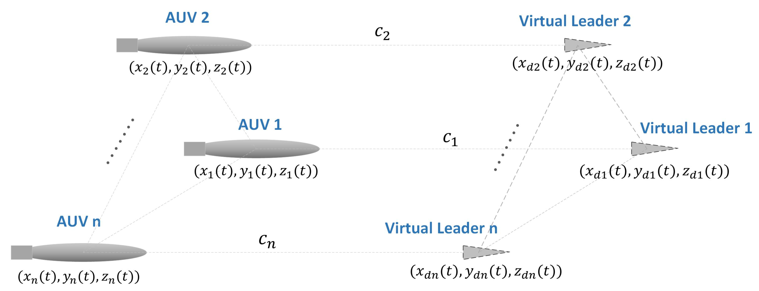
For any given continuous function f ( x ) , it always can be expressed in the following parametric form [23,24]
f ( x ) = W * T ϕ * ( x ) ,
where W * N * is a constant vector and ϕ * ( x ) N * is the basis function vector of f ( x ) . If ϕ * ( x ) can be exactly known in advance, then the functional approximation problem can be transferred to a well-known parameters estimation problem. However in practice, especially for the highly nonlinear dynamics as in (2), it is difficult, if not impossible, to exactly know their basis function vectors in advance. Therefore, in practice, it is reasonable for (8) to be rewritten as the following form [23,24]
f ( x ) = W T ϕ ( x ) + ε ( x ) ,
where ϕ ( x ) N is the constructed basis function vector and W N is the corresponding constant coefficients vector with N N * .
Using (9), the vehicle’s dynamics (7) can be rewritten as
u ˙ l i q ˙ i r ˙ i = W u l i T ϕ u l i W q i T ϕ q i W r i T ϕ r i + g a u i 0 0 0 g q i 0 0 0 q r i τ u i τ q i τ r i + d u l i d q i d r i ,
where ϕ a i N a is the constructed basis function vector for f a i and W a i N a is the corresponding coefficients vector, and d a i = d a i + ε a i . Here a { u l , q , r } .
In practice it is difficult to exactly derive the constant vectors W a i with a { u l , , q , r } in advance. Therefore, in this paper, we make the following assumption.
Assumption 2.
In (10), the constructed basis function vectors ϕ a i are known in advance and W a i are unknown constant vectors with a { u l , q , r } .
Assumption 3.
The uncertainty terms in (10) are bounded such that | d u l i | d u M , | d q i | d q M , and | d r i | d r M with d u M , d q M , d r M > 0 known constants.

3. Formation Rules

As mentioned before, in this paper we consider the formation control problem for a group of n torpedo-type underwater vehicles, all of which have the same kinematics and dynamics as (1) and (2). A surface vessel, which is equipped with a fully integrated underwater multiple vehicles simultaneous tracking and communication modem, is introduced so as to construct a sort of star-topological acoustic communication network with the vessel at the center point. According to this kind of network’s structural feature, as mentioned before in this paper we introduce a virtual school concept that is similar to the virtual structure [4] except that each node in this virtual school is taken as a virtual leader for each of specific underwater vehicle and assigned its own reference trajectory. Usually, in practice, the geometrical structure and the reference trajectories for each of the nodes in the virtual school are designed on the support vessel for the purpose to accomplish the given missions. To construct the designed formation, the strategy in this paper is simple, in that each vehicle is simply steered to follow the reference trajectory assigned to its virtual leader while avoiding possible obstacles.

3.1. Virtual School

In practice, given a mission—for example, to complete the survey on a given region using multiple underwater vehicles with the shortest search time, it is convenient to apply CPP (coverage path planning) algorithms to carry out the mission. In this case, each reference trajectory for each of the nodes (virtual leaders) in the virtual school can be designed through a properly designed CPP algorithm [6,25] with appropriate criteria such as minimizing the search time or energy consumption. The geometric structure of the virtual school can be determined by the specifications of the survey devices such as the side scan sonar or multi-beam sonar as in [26]. As mentioned before, the details of how to design this virtual school are out of the scope of this paper and could be considered in our future works.
After the design procedure is completed on the surface vessel, the virtual school information, indeed the exact reference trajectories p d i ( t ) = ( x d i ( t ) , y d i ( t ) , z d i ( t ) ) , i = 1 , , n for each of virtual leaders, is transmitted to each of the corresponding underwater vehicles through the acoustic communication modem mounted on the USV. Here p d i ( t ) can be a smooth function or a series of waypoints which can be considered as a piecewise smooth function. For each vehicle, the formation strategy is simple: just to follow its reference trajectory while avoiding possible obstacles, and in doing so the underwater formation can be constructed, see Figure 2.

3.2. Trajectory Following

For the ith vehicle, the formation control objective as mentioned before is just to follow its reference trajectory p d i ( t ) . Considering two kinematics (1) and (6), it is easy to see that for the ith vehicle’s any given trajectory p i ( t ) = ( x i ( t ) , y i ( t ) , z i ( t ) ) , it can be realized by ( u i ( t ) , v i ( t ) , w i ( t ) , θ i ( t ) , ψ i ( t ) ) through the position kinematics in (1), or also simply by the spherical coordinates ( u l i ( t ) , θ l i ( t ) , ψ l i ( t ) ) using (6). In this paper, we apply the latter method.
For the ith vehicle’s given reference trajectory p d i ( t ) = ( x d i ( t ) , y d i ( t ) , z d i ( t ) ) combined with ( θ l d i , ψ l d i ) where the kinematics is taken as (6), the position error is defined as following
p e i ( t ) = | | p d i p i | | 2 = ( x d i ( t ) x i ( t ) ) 2 + ( y d i ( t ) y i ( t ) ) 2 + ( z d i ( t ) z i ( t ) ) 2 ,
whose time derivative further can be expanded as
p ˙ e i = u l d i c o s θ l d i c o s θ b i c o s ( ψ l d i ψ b i ) + s i n θ l d i s i n θ b i u l i c o s θ l i c o s θ b i c o s ( ψ l i ψ b i ) + s i n θ l i s i n θ b i = u l d i A l d i u l i A l i ,
where θ b i and ψ b i denote the polar and azimuth angles for the position error vector p e i and are defined as follows
θ b i = a t a n ( z d i z i ) ( x d i x i ) 2 + ( y d i y i ) 2 ,
ψ b i = a t a n 2 ( y d i y i , x d i x i ) .
For the ith vehicle, the control objective of trajectory following in this paper is defined as follows.
Trajectory following objective: For the ith vehicle’s given reference trajectory ( p d i ( t ) , θ l d i ( t ) , ψ l d i ( t ) ) , the control objective is to steer the vehicle so as for ( p e i ( t ) , θ l i ( t ) , ψ l i ( t ) ) ( c i , θ b i ( t ) , ψ b i ( t ) ) where c i > 0 is a constant design parameter, see Figure 2.
Remark 4.
For the ith vehicle, since ( θ l i ( t ) , ψ l i ( t ) ) ( θ b i ( t ) , ψ b i ( t ) ) , its control strategy is clear that to force the vehicle to always face to the target point ( x d i ( t ) , y d i ( t ) , z d i ( t ) ) while keeping p e i ( t ) c i . This is why we call it trajectory following, which is different from the traditional trajectory tracking where the control objective is to ( p i ( t ) , θ l i ( t ) , ψ l i ( t ) ) ( p d i ( t ) , θ l d i ( t ) , ψ l d i ( t ) ) where θ l d i ( t ) and ψ l d i ( t ) are predefined.
Consequently, using the spherical coordinates ( u l i , θ l i , ψ l i ) and ( p e i , θ b i , ψ b i ) , the ith vehicle’s trajectory following model can be expressed as the following three-input-three-output strict-feedback form,
p ˙ e i θ ˙ l e i ψ ˙ l e i = u l d i A l d i θ ˙ b i f θ l i ψ ˙ b i f ψ l i A l i 0 0 0 g θ l i 0 0 0 g ψ l i u l i q i r i ,
u ˙ l i q ˙ i r ˙ i = W u l i T ϕ u l i W q i T ϕ q i W r i T ϕ r i + g a u i 0 0 0 g q i 0 0 0 g r i τ u i τ q i τ r i + d u l i d q i d r i ,
where θ l e i = θ b i θ l i and ψ l e i = ψ b i ψ l i .
In the case θ l e i = ψ l e i = 0 , (12) becomes p ˙ e i = u l d i u l i for which we have the following proposition.
Proposition 1
([18]). If the stabilizing function [19] for virtual input u l i is taken as
u l i = u l i R = u l d i A l d i + k p ( p e i c i ) ,
where k p > 0 is design parameter, then it can guarantee the exponential stability of p e i c i .
Proof. 
Refer to [18]. □

3.3. Obstacle Detection and Avoidance

For each vehicle, there is a forward-looking sonar mounted in front of it and used to detect obstacles. In [11,18], each detected obstacle block is modeled as the nearest point from the sonar head. Though it is simple, this kind of obstacle modeling method might cause some practical problems such as infinite wall following [27]. For this reason, this paper applies the occupancy grid map [28] to model the detected obstacles. At each time t > 0 , using the sonar measurements (multi-beam range measurements or cloud points corresponding to its current ping), we can update the related grids in the map as seen in Figure 3, and consequently, with the series of sonar ping measurements, we can construct the occupancy grid map. In the case of the occupancy grid map, it is convenient to apply the potential function method [29] to guide the vehicle to avoid obstacles. In this paper, we apply the following smooth potential function [8,11]
f p ( ζ , a ) = c o a ζ 1 τ a τ 2 ρ τ a d τ ,
where c o > 0 is a constant and ρ ( · ) is a smooth bump function taken as following form
ρ ( ξ ) = 1 , ξ [ 0 , h ) e ( ξ h ) 2 ( ξ 1 ) 2 , ξ [ h , 1 ] 0 , o t h e r w i s e
where h ( 0 , 1 ) is a design parameter. It is easy to see that f p ( ζ , a ) is a monotone decreasing function and if ζ a , then f p ( ζ , a ) = 0 .
Remark 5.
In practice, each vehicle can have its own occupancy grid map to avoid obstacles, and the grid size (or map accuracy), as well as the map size, can be adjusted according to the different mission tasks and situations.
Remark 6.
It is well known that the potential function method cannot always guarantee the global minimum in the path search [29]. In the case where the vehicle is trapped in a complicated obstacle environment, how to escape from this local minimum has been a challenging task in the past decades [30] and is also out of the scope of this paper. For the convenience of discussion, in this paper we only consider the case where the potential function method can guarantee the global minimum of path searching.

4. Formation Controller Design

Now consider the ith vehicle’s trajectory following kinematics and dynamics of (15) and (16). For this three-input-three-output strict-feedback form, it is convenient to apply the general backstepping method [19] combined with the Lyapunov direct method [20] to solve the formation control problem.
Step 1. The formation strategy in this paper is to steer the vehicle ( p i ( t ) , θ l i ( t ) , ψ l i ( t ) ) to follow its own virtual leader ( p d i ( t ) , θ l d i ( t ) , ψ l d i ( t ) ) so as for p e i ( t ) c i and ( θ l i ( t ) , ψ l i ( t ) ) ( θ b i ( t ) , ψ b i ( t ) ) . For this reason, in this step, we consider the following Lyapunov function candidate
V 1 = i = 1 n ( p e i c i ) 2 + γ θ θ l e i 2 + γ ψ ψ l e i 2 + γ O B k = 1 m f p ( p e i k , a ) ,
where γ θ , γ ψ , γ O B > 0 are weighting factors, and the smooth potential function f p ( · ) is defined as (18) with (19), and p e i k = | | p i p i k | | 2 where | | · | | 2 denotes the Euclidean norm and p i k indicates the center point of the kth grid in the ith vehicle’s occupancy grid map where the assigned value to kth grid is larger than certain pre-defined threshold.
By differentiating the above equation and substituting (15) into it, we can get
V ˙ 1 = i = 1 n ( p e i c i ) ( u l d i A l d i A l i u l i ) + γ θ θ l e i ( θ ˙ b i f θ l i g θ l i q i ) + γ ψ ψ l e i ( ψ ˙ l i f ψ l i g ψ l i r i ) + γ O B k = 1 m f p ( p e i k , a ) p e i k x i k x i p e i k ( x ˙ i k x ˙ i ) + y i k y i p e i k ( y ˙ i k y ˙ i ) + z i k z i p e i k ( z ˙ i k z ˙ i ) = i = 1 n ( p e i c i ) u l d i A l d i u l i R + u l i R u l i u l i c o s θ l i c o s θ b i ( c o s ψ l e i 1 ) + ( c o s θ l e i 1 ) + γ θ θ l e i ( θ ˙ b i f θ l i g θ l i q i ) + γ ψ ψ l e i ( ψ ˙ l i f ψ l i g ψ l i r i ) + γ O B B x i u l i R c o s θ b i c o s ψ b i u l i c o s θ l i c o s ψ l i + B y i u l i R c o s θ b i s i n ψ b i u l i c o s θ l i s i n ψ l i B z i u l i R s i n θ b i u l i s i n θ l i + Λ O B ,
where
B ζ i = k = 1 m f p p e i k ζ e i k p e i k , with ζ { x , y , z } Λ O B = γ O B i = 1 n B x i x ˙ i k u l i R c o s θ b i c o s ψ l i + B y i y ˙ i k u l i R c o s θ b i s i n ψ l i + B z i z ˙ i k + u l i R s i n θ b i .
As aforementioned, if we choose the stabilization function u l i R for virtual input u l i as (17), and let α q i and α r i denote the stabilization functions for each of virtual inputs q i and r i with e q i = α q i q i and e r i = α r i r i , then (21) can be further expanding as following
V ˙ 1 = i = 1 n k p ( p e i c i ) 2 + ( p e i c i ) u l e i + 2 u l i c o s θ l i c o s θ b i s i n 2 ψ l e i 2 + s i n 2 θ l e i 2 + γ θ θ l e i ( θ ˙ b i f θ l i g θ l i α q i + g θ l i e q i ) + γ ψ ψ l e i ( ψ ˙ b i f ψ l i g ψ l i α r i + g ψ l i e r i ) + γ O B B x i u l e i c o s θ b i c o s ψ b i 2 u l i c o s ψ b i s i n θ b i + θ l i 2 s i n θ l e i 2 + c o s θ l i s i n ψ b i + ψ l i 2 s i n ψ l e i 2 + B y i u l e i c o s θ b i s i n ψ b i 2 u l i s i n ψ b i s i n θ b i + θ l i 2 s i n θ l e i 2 c o s θ l i c o s ψ b i + ψ l i 2 s i n ψ l e i 2 B z i u l e i s i n θ b i + 2 u l i c o s θ b i + θ l i 2 s i n θ l e i 2 + Λ O B .
According to (22), the control laws for α q i and α r i are designed as follows.
α q i = g θ l i 1 θ ˙ b i f θ l i + γ θ 1 Λ θ l e i + k θ θ l e i ,
α r i = g ψ l i 1 ψ ˙ b i f ψ l i + γ ψ 1 Λ ψ l e i + k ψ ψ l e i ,
where k θ , k ψ > 0 are design parameters and
Λ θ l e i = u l i s i n θ l e i 2 θ l e i 2 ( p e i c i ) s i n θ l e i 2 γ O B B z i c o s θ b i + θ l i 2 + s i n θ b i + θ l i 2 B x i c o s ψ b i + B y i s i n ψ b i , Λ ψ l e i = u l i c o s θ l i s i n ψ l e i 2 ψ l e i 2 ( p e i c i ) c o s θ b i s i n ψ l e i 2 + γ O B B y i c o s ψ b i + ψ l i 2 B x i s i n ψ b i + ψ l i 2 .
Applying the virtual control laws (23) and (24) into (22), it has
V ˙ 1 = i = 1 n k p ( p e i c i ) 2 k θ θ l e i 2 k ψ ψ l e i 2 + Λ u l e i u l e i + γ θ θ l e i g θ l i e q i + γ ψ ψ l e i g ψ l i e r i + Λ O B ,
where Λ u l e i is defined as follows
Λ u l e i = p e i c i + γ O B B x i c o s θ b i c o s ψ b i + B y i c o s θ b i s i n ψ b i B z i s i n θ b i .
Step 2. Recall the ith vehicle’s dynamics (16) and rewriting it in the error terms as following
u ˙ l e i e ˙ q i e ˙ r i = u ˙ l i R W u l i T ϕ u l i α ˙ q i W q i T ϕ q i α ˙ r i W r i T ϕ r i g a u i 0 0 0 g q i 0 0 0 g r i τ u i τ q i τ r i d u l i d q i d r i .
The following Lyapunov function candidate is applied in this step,
V 2 = V 1 + 1 2 i = 1 n γ u u l e i 2 + γ q e q i 2 + γ r e r i 2 ,
where γ u , γ q , γ r > 0 are weighting factors.
By differentiating (27) and further substituting (25) and (26) into it, we can get the following expansion
V ˙ 2 = i = 1 n k p ( p e i c i ) 2 k θ θ l e i 2 k ψ ψ l e i 2 + Λ u l e i u l e i + γ θ θ l e i g θ l i e q i + γ ψ ψ l e i g ψ l i e r i + γ u u l e i u ˙ l i R W u l i T ϕ u l i g a u i τ u i d u l i + γ q e q i α ˙ q i W q i T ϕ q i g q i τ q i d q i + γ r e r i α ˙ r i W r i T ϕ r i g r i τ r i d r i + Λ O B .
According to the above equation, the control laws in Step 2 are chosen as following
τ u i = g a u i 1 u ˙ l i R W ^ u l i T ϕ u l i + d u M η γ u u l e i d u M + γ u 1 ( k u u l e i + Λ u l e i ) ,
τ q i = g q i 1 α ˙ q i W ^ q i T ϕ q i + d q M η γ q e q i d q M + γ q 1 ( k q e q i + γ θ θ l e i g θ l i ) ,
τ r i = g r i 1 α ˙ r i W ^ r i T ϕ r i + d r M η γ r e r i d r M + γ r 1 ( k r e r i + γ ψ ψ l e i g ψ l i ) ,
where W ^ a i with a { u l , q , r } is the estimation of W a i , k u , k q , k r > 0 are design parameters, and function η ( · ) denotes a smooth function and satisfies the following proposition.
Proposition 2
([22]). ϵ > 0 , there is a smooth function η ( · ) such that η ( 0 ) = 0 and
| ξ | ξ η ( ξ ) + ϵ , ξ .
Remark 7
([22]). One of the example functions satisfying Proposition 2 is η ( ξ ) = t a n h ( κ ξ / ϵ ) with κ = e ( κ + 1 ) .
By applying the above control laws into (28), we can get
V ˙ 2 i = 1 n k p ( p e i c i ) 2 k θ θ l e i 2 k ψ ψ l e i 2 k u u l e i 2 k q e q i 2 k r e r i 2 γ u u l e i W ˜ u l i T ϕ u l i + γ u | u l e i d u l i | γ u u l e i d u M η γ u u l e i d u M γ q e q i W ˜ q i T ϕ q i + γ q | e q i d q i | γ q e q i d q M η γ q e q i d q M γ r e r i W ˜ r i T ϕ r i + γ r | e r i d r i | γ r e r i d r M η γ r e r i d r M + Λ O B ,
where W ˜ a i = W a i W ^ a i with a { u l , q , r } denote the estimation errors.
Applying Proposition 2, (33) can be expanded as following
V ˙ 2 i = 1 n k p ( p e i c i ) 2 k θ θ l e i 2 k ψ ψ l e i 2 k u u l e i 2 k q e q i 2 k r e r i 2 γ u u l e i W ˜ u l i T ϕ u l i γ q e q i W ˜ q i T ϕ q i γ r e r i W ˜ r i T ϕ r i + ϵ u i + ϵ q i + ϵ r i + Λ O B .
Now we consider the following final step Lyapunov function candidate
V 3 = V 2 + 1 2 i = 1 n W ˜ u l i T Γ u l W ˜ u l i + W ˜ q i T Γ q W ˜ q i + W ˜ r i T Γ r W ˜ r i ,
where Γ a N a × N a with a { u l , q , r } are strictly positive definite matrix.
By differentiating (35) and substituting (34) into it, we can get
V ˙ 3 i = 1 n k p ( p e i c i ) 2 k θ θ l e i 2 k ψ ψ l e i 2 k u u l e i 2 k q e q i 2 k r e r i 2 + ϵ u i + ϵ q i + ϵ r i γ u u l e i W ˜ u l i T ϕ u l i W ˜ u l i T Γ u l W ^ ˙ u l i γ q e q i W ˜ q i T ϕ q i W ˜ q i T Γ q W ^ ˙ q i γ r e r i W ˜ r i T ϕ r i W ˜ r i T Γ r W ^ ˙ r i + Λ O B .
Here we choose the online adaptation laws for the ith vehicle’s hydrodynamic coefficients as follows
W ^ ˙ u l i = Γ u l 1 γ u u l e i ϕ u l i + k W u W ^ u l i W u l o ,
W ^ ˙ q i = Γ q 1 γ q e q i ϕ q i + k W q W ^ q i W q o ,
W ^ ˙ r i = Γ r 1 γ r e r i ϕ r i + k W r W ^ r i W r o ,
where k W u , k W q , k W r > 0 are design parameters, and W a o with a { u l , q , r } are the initial values of W ^ a i at t = 0 .
Substituting (37)–(39) into (36), finally we can get
V ˙ 3 i = 1 n k p ( p e i c i ) 2 k θ θ l e i 2 k ψ ψ l e i 2 k u u l e i 2 k q e q i 2 k r e r i 2 1 2 k W u W ˜ u l i T W ˜ u l i 1 2 k W q W ˜ q i T W ˜ q i 1 2 k W r W ˜ r i T W ˜ r i + ϵ u i + ϵ q i + ϵ r i + E W i + Λ O B ,
where E W i = k W u | | W u l i W u l o | | 2 2 + k W q | | W q i W q o | | 2 2 + k W r | | W r i W r o | | 2 2 / 2 .
As mentioned in Remark 6, in this paper we only consider the case where the potential function method of obstacle avoidance can guarantee the global minimum of path searching. Therefore, after a certain period of time, the vehicles always escape from the obstacles. Let us recall the potential function defined as (18). In the case after the vehicles are all escaped from the obstacles, we have i , k , | | p e i k | | 2 a , therefore f p ( p e i k , a ) = 0 , and f p ( p e i k , a ) / p e i k = 0 . This means that B ζ i = 0 with ζ { x , y , z } . Consequently we get Λ O B = 0 and (40) becomes
V ˙ 3 λ V 3 + ρ ,
with λ and ρ defined as following
λ = m i n 2 k p , 2 k θ γ θ 1 , 2 k ψ γ ψ 1 , 2 k u γ u 1 , 2 k q γ q 1 , 2 k r γ r 1 , k W u λ m i n 1 ( Γ u l ) , k W q λ m i n 1 ( Γ q ) , k W r λ m i n 1 ( Γ r ) ,
ρ = ϵ u i + ϵ q i + ϵ r i + E W i ,
where λ m i n ( Γ ) indicates the minimum singular value of matrix Γ .
Theorem 1.
Considering the formation control of multiple underactuated underwater vehicles whose kinematics and dynamics are taken as (1) and (2) with Assumption 1–3, if we choose the formation control laws as (29)–(31) and the vehicles’ hydrodynamics coefficients adaptation laws as (37)–(39), then we can guarantee the uniform ultimate boundedness (UUB) of closed-loop system in terms of spherical coordinates.
Proof. 
From (41), it is easy to verify that
0 V 3 ( t ) V 3 ( 0 ) ρ λ e λ t + ρ λ ,
which indicates that V 3 ( t ) will exponentially converge to ρ / λ and this concludes the proof. □
Remark 8.
In the case where the basis function vectors ϕ u l i , ϕ q i , and ϕ r i satisfy to be persistency excitation, the adaptation laws (37)–(39) with k W u = k W q = k W r = 0 can guarantee the exact estimation of W u l i , W q i , and W r i . Unfortunately, this kind of PE conditions are difficult to be satisfied in most of practical applications, and in this case, properly designed parameters k W u = k W q = k W r > 0 can prevent the divergence of W ^ u l i , W ^ q i , and W ^ r i [22,24].
Remark 9.
Consider the definition of the polar and azimuth angles θ b i and ψ b i as in (13) and (14). It is easy to see that if p e i = 0 , then both of θ b i and ψ b i are undefined. Here the properly designed parameters c i > 0 in practice so as for p e i c i can prevent the above mentioned singularity problem.

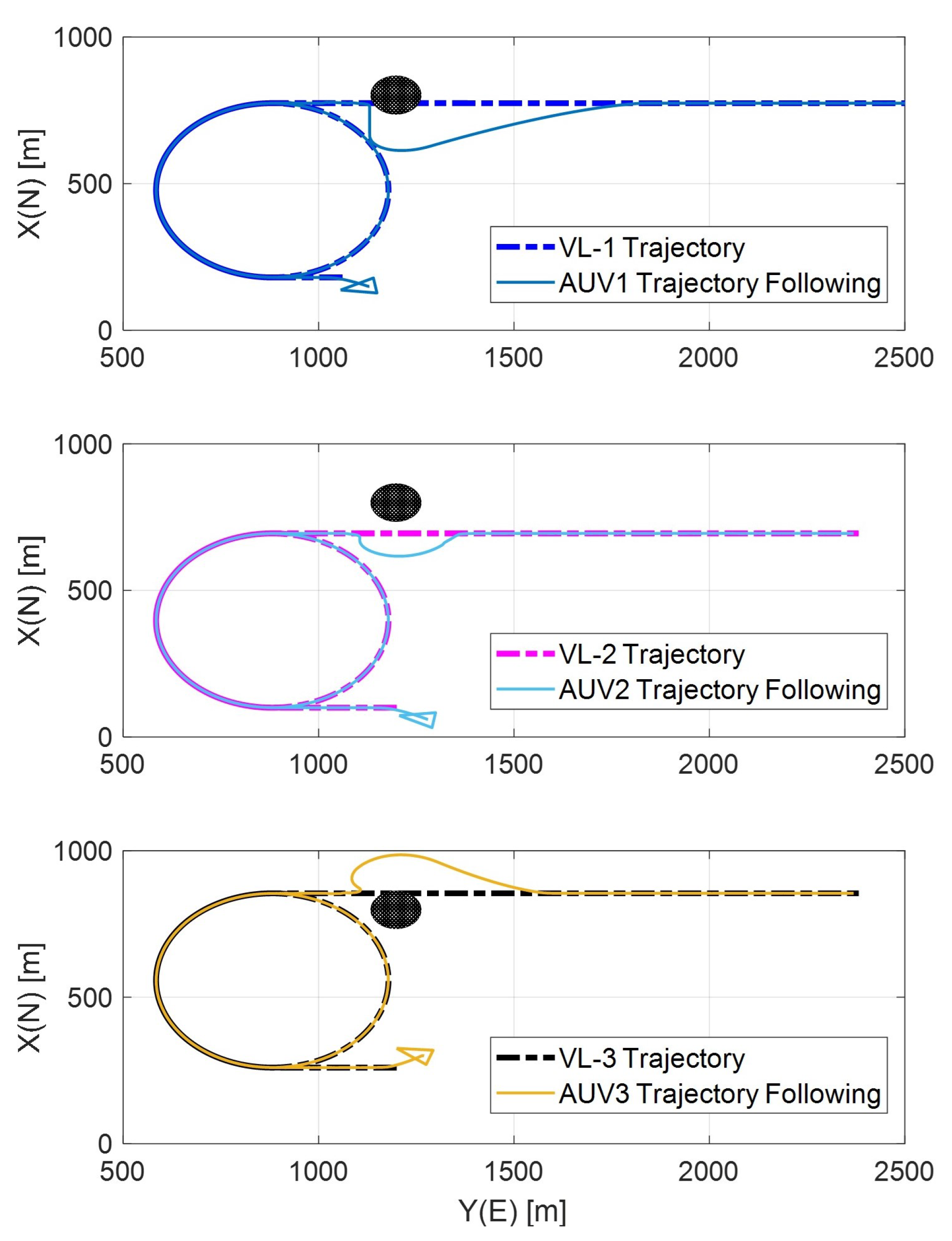
5. Numerical Studies

To verify the effectiveness of the proposed formation scheme, in this section we carry out some simulation studies using the 6-DOF of REMUS AUV simulation model [31]. In the simulation, both the rudder and stern plane angles are saturated by 15 degrees.
There was a total of three vehicles with the same dynamics considered in the simulation, and the trajectories for each virtual leader are designed as follows. For Virtual Leader 1, if t < 120 s, then u l d 1 = 1.5 m/s, and θ ˙ l d 1 = ψ ˙ l d 1 = 0 ; else if t < 2000 s, then u l d 1 = 1.5 m/s, θ ˙ l d 1 = 0.1337 , and ψ ˙ l d 1 = 0.005 ; else, u l d 1 = 1.5 m/s, and θ ˙ l d 1 = ψ ˙ l d 1 = 0 . For both of Virtual Leader 2 and 3, if t < 212 s, then u l d i = 1.5 m/s, and θ ˙ l d i = ψ ˙ l d i = 0 ; else if t < 2100 s, then u l d i = 1.5 m/s, θ l d i = 0.1337 rad, and ψ ˙ l d i = 0.005 rad/s; else, u l d i = 1.5 m/s, and θ ˙ l d i = ψ ˙ l d i = 0 with i = 2 , 3 . And the initial conditions are set as: p d 1 ( 0 ) = ( 180 m , ( 1200 3 ) m , 200 m ) , p d 2 ( 0 ) = ( 100 m , 1200 m , 200 m ) , p d 3 ( 0 ) = ( 260 m , 1200 m , 200 m ) , ψ l d i = 90 degrees , i = 1 , 2 , 3 . Three vehicles initial conditions are chosen as: X 1 ( 0 ) = ( 150 m , 1130 m , 220 m , 0 , 0 , 100 deg , 0.5 m / s , 0 , 0 , 0 , 0 , 0 ) , X 2 ( 0 ) = ( 60 m , 1280 m , 200 m , 0 , 0 , 80 deg , 0.5 m / s , 0 , 0 , 0 , 0 , 0 ) , and X 3 ( 0 ) = ( 300 m , 1270 m , 180 m , 0 , 0 , 70 deg , 0 , 0 , 0 , 0 , 0 ) where X = ( x , y , z , ϕ , θ , ψ , u , v , w , p , q , r ) .
The controller design parameters are chosen as: c = 15 ; k p = 1 , k u = 15 , k θ = 15000 , k ψ = 6000 , k q = 120 , k r = 2000 ; γ u = 14 , γ θ = 200 , γ ψ = 200 , γ O B = 20 , γ q = 60 , γ r = 10 ; Γ u l = 5 d i a g ( o n e s ( 25 , 1 ) ) , Γ q = d i a g ( o n e s ( 11 , 1 ) ) , Γ r = d i a g ( o n e s ( 7 , 1 ) ) , k W u = 8 , k W q = k W r = 0.1 , W u l o = 0.5 W u l i , W q o = 0.5 W q i , W r o = 0.5 W r i . Corresponding to the smooth potential function (18) and bump function (19), we set c o = 3 , a = 200 , and h = 0.9 . And the disturbance terms are selected as d u i = 1.5 ( 1 2 r a n d ) , d v i = 0.5 ( 1 2 r a n d ) , d w i = 0.5 ( 1 2 r a n d ) , d q i = 0.3 ( 1 2 r a n d ) , and d r i = 0.3 ( 1 2 r a n d ) . Finally, the obstacle is modeled as follows
z = 600 100 c o s π 0.01 ( x x o ) 2 + ( y y o ) 2 ,
where ( x o , y o ) = ( 800 m , 1200 m ) .
Simulation results are shown in Figure 4, Figure 5, Figure 6 and Figure 7. Figure 4 and Figure 5 show the virtual leaders’ designed trajectories and the vehicles’ corresponding trajectory following results while avoiding the given obstacle, from which we can see that the proposed formation scheme can provide satisfactory trajectory following performance while properly avoiding the obstacles. Figure 6 shows the corresponding trajectory following errors in terms of spherical coordinates, and we can see that all the error terms are bounded except during the obstacle avoidance and this is coincident with the main result of this paper. Considering the adaptation laws (37)–(39), it might be interesting to investigate their coefficients estimations performance, and Figure 7 shows the result, from which we can see that the adaptation laws cannot guarantee the exact estimation of coefficients under this simulation conditions. However, the adaptation laws still can prevent the divergence of estimations.

6. Conclusions

An adaptive formation control scheme for a group of torpedo-type underactuated AUVs has been presented in this paper by introducing a sort of virtual school concept. This virtual school, which is similar to the virtual structure, is a geometric graph where each node is taken as a virtual leader for each specific AUV and assigned its own reference trajectory. The formation strategy is that each vehicle is forced to follow its virtual leader so as to construct the pre-defined formation. Since the individual vehicle considered in this paper is a torpedo-type underactuated system, another main focus in this paper has been on the trajectory following the controller design problem for each vehicle. The proposed adaptive formation control scheme can guarantee the UUB of a closed-loop system in terms of spherical coordinates. Numerical simulations also have been carried out and presented the effectiveness of the proposed method.
As mentioned before, the main focus of this paper is formation tracking rather than formation producing [1]. Therefore, how to properly design the formation structure for multiple underactuated underwater vehicles might be one of our most interesting future works. On the other hand, during the simulation studies, we have found that the potential functions shown in (18) seem not very efficient in obstacle avoidance. So, finding a more efficient potential function for obstacle avoidance also requires further study.

Author Contributions

Conceptualization, J.-H.L. and M.-J.L.; Data curation, H.K., M.-G.K., and M.-J.L.; Funding acquisition, J.-H.L.; Methodology, J.-H.L. and G.R.C.; Resources, H.K., M.-G.K., and H.-S.J.; Supervision, J.-H.L.; Validation, H.-S.J.; Writing—original draft, J.-H.L. All authors have read and agreed to the published version of the manuscript.

Funding

This work is partially supported by the project titled “AUV Fleet and its Operation System Development for Quick Response of Search on Maritime Disasters” of Korea Institute of Marine Science & Technology Promotion (KIMST) funded by the Korea Coast Guard Agency (KIMST-20210547); also was a part of the project titled “Development of Unmanned Remotely Construction Aided System for Harbor Infrastructure”, and funded by the Ministry of Oceans and Fisheries, Republic of Korea.

Institutional Review Board Statement

Not applicable.

Informed Consent Statement

Not applicable.

Conflicts of Interest

The authors declare no conflict of interest.

References

  1. Ren, W.; Cao, Y. Distributed Coordination of Multi-Agent Networks: Emergent Problems, Models, and Issues; Springer: London, UK, 2010. [Google Scholar]
  2. Chen, Y.; Wang, Z. Formation control: A review and a new consideration. In Proceedings of the IEEE/RSJ International Conference on Intelligent Robots and Systems, Edmonton, AB, Canada, 2–6 August 2005. [Google Scholar]
  3. Oh, K.K.; Park, M.C.; Ahn, H.S. A survey of multi-agent formation control. Automatica 2015, 53, 424–440. [Google Scholar]
  4. Lewis, M.A.; Tan, K.H. High Precision Formation Control of Mobile Robots Using Virtual Structures. Auton. Robot. 1997, 4, 387–403. [Google Scholar] [CrossRef]
  5. Beard, R.W.; Lawton, J.; Hadaegh, F.Y. A coordination architecture for spacecraft formation control. IEEE Trans. Control Syst. Technol. 2001, 9, 777–790. [Google Scholar]
  6. Galceran, E.; Carreras, M. A survey on coverage path planning for robotics. Robot. Auton. Syst. 2013, 61, 1258–1276. [Google Scholar]
  7. Reynolds, C.W. A distributed behavioral model. In Proceedings of the ACM SIGGRAPH’87, Anaheim, CA, USA, 27–31 July 1987. [Google Scholar]
  8. Olfati-Saber, R.; Murray, R.M. Distributed cooperative control of multiple vehicle formations using structural potential functions. In Proceedings of the 15th IFAC World Congress, Barcelona, Spain, 21–26 July 2002. [Google Scholar]
  9. Fax, J.A.; Murray, R.M. Information flow and cooperative control of vehicle formation. IEEE Trans. Autom. Control 2004, 49, 1465–1476. [Google Scholar] [CrossRef]
  10. Yan, Z.; Jiang, A.; Lai, C. Adaptive Formation Control of Unmanned Underwater Vehicles with Collision Avoidance under Unknown Disturbances. J. Mar. Sci. Eng. 2022, 10, 516. [Google Scholar] [CrossRef]
  11. Li, J.H.; Jun, B.H.; Lee, P.M.; Lim, Y.K. Schooling for multiple underwater AUVs. In Underwater Vehicles; InTech: Vienna, Austria, 2009; pp. 295–314. [Google Scholar]
  12. Cui, R.; Ge, S.S.; How, B.V.; Choo, Y.S. Leader-follower formation control of underactuated autonomous underwater vehicles. Ocean Eng. 2010, 37, 1491–1502. [Google Scholar] [CrossRef]
  13. Park, B.S. Adaptive formation control of underactuated autonomous underwater vehicles. Ocean Eng. 2015, 96, 1–7. [Google Scholar] [CrossRef]
  14. Li, H.; Xie, P.; Yan, W. Receding Horizon Formation Tracking Control of Constrained Underactauted Autonomous Underwater Vehicles. IEEE Trans. Ind. Electron. 2017, 64, 5004–5012. [Google Scholar] [CrossRef]
  15. Li, J.; Du, J.; Chang, W.J. Robust time-varying formation control for underactuated autonomous underwater vehicles with disturbances under input saturation. Ocean Eng. 2019, 179, 180–188. [Google Scholar] [CrossRef]
  16. Gao, Z.; Guo, G. Velocity free leader-following formation control for autonomous underwater vehicles with line-of-sight range and angle constraints. Inf. Sci. 2019, 486, 359–378. [Google Scholar] [CrossRef]
  17. Qi, X.; Cai, Z.J. Three-dimensional formation control based on nonlinear small gain method for multiple underactuated underwater vehicles. Ocean Eng. 2018, 151, 105–114. [Google Scholar]
  18. Li, J.H.; Park, D.; Kang, H.; Cho, G.R. 3D formation control of multiple torpedo-type underactuated AUVs. In Proceedings of the 21st IFAC World Congress, Berlin, Germany, 12–17 July 2020. [Google Scholar]
  19. Krstic, M.; Kanellakopoulos, I.; Kokotovic, P. Nonlinear and Adaptive Control Design; John Wiley & Sons Inc.: New York, NY, USA, 1995. [Google Scholar]
  20. Slotine, J.E.; Li, W. Applied Nonlinear Control; Prentice-Hall Inc.: Englewood Cliffs, NJ, USA, 1991. [Google Scholar]
  21. Fossen, T.I. Handbook of Marine Craft Hydrodynamics and Motion Control; John Wiley & Sons. Ltd.: Hoboken, NJ, USA, 2011. [Google Scholar]
  22. Li, J.H.; Lee, M.J.; Kang, H.; Kim, M.G.; Cho, G.R. Neural-Net based Robust Adaptive Control for 3D Path Following of Torpedo-type AUVs. In Proceedings of the 59th IEEE Conference on Decision and Control (CDC), Jeju Island, Korea, 14–18 December 2020. [Google Scholar]
  23. Giori, F.; Poggio, T. Networks and the Best Approximation Property. Biol. Cybern. 1990, 63, 169–176. [Google Scholar]
  24. Li, J.H.; Lee, P.M. Neural Network Adaptive Control for a Class of Nonlinear Systems with Unknown-Bound Unstructured Uncertainties. In Proceedings of the 43rd IEEE Conference on Decision and Control, Paradise Island, Bahamas, 14–17 December 2004. [Google Scholar]
  25. Collins, L.; Ghassemi, P.; Esfahani, E.T.; Doermann, D.; Dantu, K.; Chowdhury, S. Scalable Coverage Path Planning of Multi-Robot Teams for Monitoring Non-Convex Areas. In Proceedings of the 2021 IEEE International Conference on Robotics and Automation, Xi’an, China, 31 May–4 June 2021. [Google Scholar]
  26. Kapetanovic, N.; Miskovic, N.; Tahirovic, A.; Kvasic, I. Side-Scan Sonar Data-Driven Coverage Path Planning: A Comparison of Approaches. In Proceedings of the MTS/IEEE Oceans 2019 Marseille, Marseille, France, 17–20 June 2019. [Google Scholar]
  27. Li, J.H.; Kang, H.; Park, G.H.; Suh, J.H. Real Time Path Planning of Underwater Robots in Unknown Environment. In Proceedings of the 2017 International Conference on Control, Artificial Intelligence, Robotics & Optimization, Prague, Czech Republic, 20–22 May 2017. [Google Scholar]
  28. Thurn, S.; Burgard, W.; Fox, D. Probabilistic Robotics; The MIT Press: Cambridge, MA, USA, 2005. [Google Scholar]
  29. Latombe, J.C. Robot Motion Planning; Kluwer Academic Publisher: Dordrecht, The Netherlands, 1991. [Google Scholar]
  30. Russell, S.; Norvig, P. Artificial Intelligence, A Mordern Approach, 4th ed.; Pearson Education, Inc.: Upper Saddle River, NJ, USA, 2021. [Google Scholar]
  31. Prestero, T. Verification of a Six-Degree of Freedom Simulation Model for the REMUS Autonomous Underwater Vehicles. Master’s Thesis, Department of Ocean Engineering and Mechanical Engineering, MIT, Cambridge, MA, USA, 2001. [Google Scholar]
Figure 1. Star-topological acoustic communication network for a group of AUVs and a USV.
Jmse 10 01233 g001
Figure 2. Virtual structure based multiple AUVs schooling.
Jmse 10 01233 g002
Figure 3. Obstacle detection and its modeling using occupancy grid map.
Jmse 10 01233 g003
Figure 4. Virtual leaders trajectories and their trajectory with obstacle avoidance using the proposed formation scheme.
Jmse 10 01233 g004
Figure 5. Each vehicle’s trajectory following with obstacle avoidance on the horizontal plane.
Jmse 10 01233 g005
Figure 6. UUB stability of proposed formation scheme in terms of spherical coordinate frame.
Jmse 10 01233 g006
Figure 7. Some of coefficients estimations using the adaptation laws (37)–(39).
Jmse 10 01233 g007
Publisher’s Note: MDPI stays neutral with regard to jurisdictional claims in published maps and institutional affiliations.

