Application of the Trigonometric Polynomial Interpolation for the Estimation of the Vertical Eddy Viscosity Coefficient Based on the Ekman Adjoint Assimilation Model

Abstract

In this study, a triangular polynomial interpolation (TPI) scheme was developed to estimate the vertical eddy viscosity coefficient (VEVC) on the basis of the Ekman model with adjoint assimilation. In the twin experiments, the advantages and disadvantages of estimating the VEVC using the TPI scheme under different factors are discussed. The results indicated that (1) the TPI scheme proves to be better than the cubic spline interpolation (CSI) and Cressman interpolation (CI) schemes; (2) the inversion results are more sensitive to observations from upper ocean layers than those from lower layers, and the TPI scheme is less likely to be influenced by missing data; (3) for various boundary layer depths, the inversion results of the TPI scheme remain consistent with the given distributions; (4) the inversion results can be influenced considerably by observational errors, and the TPI scheme is more resistant to noise than the CSI and CI schemes; and (5) the inversion accuracy of the TPI scheme can be improved by selecting the temporal wind stress drag coefficients. In practical experiments, the adjoint method with the TPI scheme was developed to estimate the Ekman currents by assimilating the observations from a buoy stationed in the Yellow Sea. The results showed the successful estimation of the VEVC and demonstrated that more precise current velocities can be obtained with this estimation scheme. In summary, this study provides a useful approach for the effective estimation of the VEVC.

1. Introduction

The eddy viscosity coefficient is a key parameter in the viscosity term, which is closely related to the turbulent structure of the ocean, and it is important for the exchange of momentum and energy between eddies and for describing internal fluid friction [1,2,3,4]. Therefore, the determination of the eddy viscosity coefficient is of key importance for understanding ocean dynamics, especially for numerical simulations of Ekman currents and turbulent mixing [5,6,7,8,9]. Whether the traditional Ekman theory, a fundamental theory in oceanography, can be observed in situ has been the subject of continuous research [10,11,12,13,14]. These studies suggested that the classical vertical eddy viscosity is inadequate and in need of improvement. Therefore, it is of great importance to parameterize the vertical eddy viscosity coefficient (VEVC). Since the VEVC is difficult to measure directly, it is usually calculated on the basis of turbulence models, such as the Prandtl mixed-length model, M-Y model, k-ε model, Richardson number, and KPP model [15,16,17,18,19]. However, in most complex turbulence models, many parameters need to be assigned. The determination of these parameters is often difficult, particularly when turbulent observations are missing or of poor quality, leading to considerable limitations in the application and accuracy of turbulence models. In addition, turbulence can be rather complex to model at various temporal ranges and spatial scales. As mentioned above, the non-universality of turbulence models is a difficult problem.

In this study, the adjoint assimilation method based on optimal control theory and variational principles was adopted to optimize the observationally derived VEVC. As an advanced data assimilation technique, the advantage of adjoint assimilation is that time- and space-varying observations can be directly assimilated into a numerical model while maintaining consistency with the model in terms of its dynamics and physics [20]. Therefore, the method has been widely used in previous studies. For example, on the basis of the Ekman model, Yu and O’Brien [21], Zhang et al. [1], and Cao et al. [22] used the adjoint method to estimate VEVCs by assimilating in situ values or those obtained by pseudo measurements. Yoshikawa et al. [23] estimated the VEVC by solving the Ekman balance equations using the least-squares method. Yoshikawa and Endoh [24] estimated the tidally induced VEVC by solving the Ekman balance equations via the velocity spiral measured. The time-varying eddy viscosity coefficients were estimated using the adjoint assimilation model by Zhang et al. [25]. In the above studies, the optimization of relevant parameters in the model often required multiple iterations.

Some interpolation schemes are frequently used to improve the operational efficiency and accuracy of the parameter estimation in the Ekman model [26,27,28]. For example, Cressman (CI) and cubic spline interpolation (CSI) schemes based on independent point (IP) methods take the VEVCs at certain selected IPs as control variables and interpolate between those IPs to calculate the VEVCs at the other points. However, the resulting distribution of the VEVC obtained by CI schemes is not smooth. Even with the CSI scheme, the number of IPs still needs to be considered. Determining the number of points often requires repeated experiments. Therefore, the trigonometric polynomial interpolation (TPI) scheme, which has the advantages of being easy to operate and not requiring the consideration of IPs and interpolation radii, was used in this work.

The structure of this paper is as follows. Section 2 introduces the numerical model and the TPI scheme. The feasibility and superiority of the TPI scheme were verified by five sets of twin experiments, as presented in Section 3. Section 4 describes how the inverted effect of the TPI scheme was verified by carrying out real-world or practical experiments. Section 5 presents the conclusions of this work.

2. Model and Estimation Scheme

2.1. Forward Model

The Ekman wind current is a pervasive and fundamental flow in the ocean, a constant flow that occurs when constant winds act over an infinite expanse of the sea surface for a long time. The Ekman layer model based on Ekman’s theory is a textbook classic and is mathematically easy to analyze, which makes it a good starting point for studying the physics of the upper layers of the ocean [12]. The model is generally built on the basis of the assumption of considering a horizontal unbounded ocean surface layer with depth H₀.

The Ekman model has been widely used to study the physical processes in the ocean’s upper layers [12]. In this study, the modified Ekman model was used to invert the VEVCs. The governing equations are as follows:

$$\left\{\begin{array}{}\frac{\partial \mathit{u}}{\partial \mathit{t}}-\mathit{f}\mathit{v}=\frac{\partial }{\partial \mathit{z}}\left(\mathit{A}\frac{\partial \mathit{u}}{\partial \mathit{z}}\right),\frac{\partial \mathit{v}}{\partial \mathit{t}}+\mathit{f}\mathit{u}=\frac{\partial }{\partial \mathit{z}}\left(\mathit{A}\frac{\partial \mathit{v}}{\partial \mathit{z}}\right).\end{array}\right.$$

(1)

The initial conditions are as follows:

$${\left.\mathit{u}\right|}_{\mathit{t}=0}={\mathit{u}}_0\mathbf{,} {\left.\mathit{v}\right|}_{\mathit{t}=0}={\mathit{v}}_0\mathbf{.}$$

(2)

The boundary conditions are as follows:

$${\left.\frac{\mathit{\partial }\mathit{u}}{\mathit{\partial }\mathit{z}}\right|}_{\mathit{z}=0}=\frac{{\mathit{C}}_{\mathit{d}}}{\mathit{A}}\mathbf{\cdot }\frac{{\mathit{\rho }}_{\mathit{a}}}{{\mathit{\rho }}_{\mathit{w}}}\sqrt{{\mathit{u}}_{\mathit{a}}^2\mathbf{+}{\mathit{v}}_{\mathit{a}}^2}{\mathit{u}}_{\mathit{a}}\mathbf{,} {\left.\frac{\mathit{\partial }\mathit{v}}{\mathit{\partial }\mathit{z}}\right|}_{\mathit{z}=0}=\frac{{\mathit{C}}_{\mathit{d}}}{\mathit{A}}\mathbf{\cdot }\frac{{\mathit{\rho }}_{\mathit{a}}}{{\mathit{\rho }}_{\mathit{w}}}\sqrt{{\mathit{u}}_{\mathit{a}}^2\mathbf{+}{\mathit{v}}_{\mathit{a}}^2}{\mathit{v}}_{\mathit{a}}\mathbf{.}$$

(3)

$$\mathit{A}{\left.\frac{\mathit{\partial }\mathit{u}}{\mathit{\partial }\mathit{z}}\right|}_{\mathit{z}=-{\mathit{H}}_0}=0\mathbf{,} \mathit{A}{\left.\frac{\mathit{\partial }\mathit{v}}{\mathit{\partial }\mathit{z}}\right|}_{\mathit{z}=-{\mathit{H}}_0}=0\mathbf{.}$$

(4)

In the equations above, $u\left(z\right)$, which is positive to the east, and $v\left(z\right)$, which is positive to the north, both refer to the horizontal current components. $t$ represents time. $z$ represents water depth and is equal to $0$ at the sea surface and negative below. In this model, the Coriolis parameter, $f$, is set as a constant. $u_a$ and $v_a$ are the wind velocity components. C_d is the wind stress drag coefficient, while A denotes the eddy viscosity coefficient. ${\rho }_a$ is the density of air, and ${\rho }_w$ is the density of the seawater. $H_0$ represents the Ekman layer’s total depth.

2.2. Adjoint Model

A cost function to quantify the difference between the simulated results and the observed results can be specified as follows:

$$\mathit{J}\left(\mathit{u}\mathbf{,}\mathit{v}\mathbf{,}\mathit{A}\mathbf{,}{\mathit{C}}_{\mathit{d}}\right)=\frac{1}{2}\mathit{K}{\displaystyle {\mathbf{\int }}_{\mathit{t}}{\displaystyle {\mathbf{\int }}_{\mathit{z}}({(\mathit{u}-\widehat{\mathit{u}})}^2\mathbf{+}{(\mathit{v}-\widehat{\mathit{v}})}^2)\mathit{d}\mathit{z}\mathit{d}\mathit{t}}}\mathbf{,}$$

(5)

where the carets denote values derived through observation. $K$ is a weighting factor, set to 1 in this study [20]. The control equations and their initial boundary value conditions can be calculated by introducing a set of Lagrange multipliers, to be determined below, and are actually adjoint variables. This results in the Lagrangian function, given by the following:

$$\begin{array}{l}\mathit{L}(\mathit{u}\mathbf{,}\mathit{v}\mathbf{,}\mathit{A}\mathbf{,}{\mathit{C}}_{\mathit{d}}\mathbf{,}\mathit{\lambda }\mathbf{,}\mathit{\mu })=\mathit{J}\mathbf{+}\\ {\displaystyle {\mathbf{\int }}_{\mathit{t}}{\displaystyle {\mathbf{\int }}_{\mathit{z}}[\mathit{\lambda }(\frac{\mathbf{\partial }\mathit{u}}{\mathbf{\partial }\mathit{t}}-\mathit{f}\mathit{v}-\frac{\mathbf{\partial }}{\mathbf{\partial }\mathit{z}}(\mathit{A}\frac{\mathbf{\partial }\mathit{u}}{\mathbf{\partial }\mathit{z}}))\mathbf{+}\mathit{\mu }(\frac{\mathbf{\partial }\mathit{v}}{\mathbf{\partial }\mathit{t}}\mathbf{+}\mathit{f}\mathit{u}-\frac{\mathbf{\partial }}{\mathbf{\partial }\mathit{z}}(\mathit{A}\frac{\mathbf{\partial }\mathit{v}}{\mathbf{\partial }\mathit{z}})]\mathit{d}\mathit{z}\mathit{d}\mathit{t}}}\mathbf{,}\end{array}$$

(6)

where $\mu$ and $\lambda$ are the Lagrange multipliers of $v$ and $u$, respectively. The intent is to minimize the cost function under the initial boundary value conditions. Therefore, when the Lagrangian function gradients are equal to zero, the following adjoint equations can be derived as follows:

$$\begin{array}{l}\frac{\mathbf{\partial }\mathit{\lambda }}{\mathbf{\partial }\mathit{t}}-\mathit{f}\mathit{\mu }\mathbf{+}\frac{\mathbf{\partial }}{\mathbf{\partial }\mathit{z}}(\mathit{A}\frac{\mathbf{\partial }\mathit{\lambda }}{\mathbf{\partial }\mathit{z}})={\mathit{K}}_{\mathit{m}}(\mathit{u}-\widehat{\mathit{u}})\mathbf{,}\\ \frac{\mathbf{\partial }\mathit{\mu }}{\mathbf{\partial }\mathit{t}}\mathbf{+}\mathit{f}\mathit{\lambda }\mathbf{+}\frac{\mathbf{\partial }}{\mathbf{\partial }\mathit{z}}(\mathit{A}\frac{\mathbf{\partial }\mathit{\mu }}{\mathbf{\partial }\mathit{z}})={\mathit{K}}_{\mathit{m}}(\mathit{v}-\widehat{\mathit{v}})\mathbf{.}\end{array}$$

(7)

The corresponding initial boundary value conditions are as follows:

$$\mathit{\lambda }{\mathbf{|}}_{\mathit{t}=\mathit{T}}=0\mathbf{,}\begin{array}{cc}& \end{array}\mathit{\mu }{\mathbf{|}}_{\mathit{t}=\mathit{T}}=0\mathbf{,}$$

(8)

$${\left.\frac{\mathbf{\partial }\mathit{\lambda }}{\mathbf{\partial }\mathit{z}}\right|}_{\mathit{z}=0}=0\mathbf{,}\begin{array}{cc}& \end{array}{\left.\frac{\mathbf{\partial }\mathit{\mu }}{\mathbf{\partial }\mathit{z}}\right|}_{\mathit{z}=0}=0\mathbf{,}$$

(9)

$${\left.\frac{\mathbf{\partial }\mathit{\lambda }}{\mathbf{\partial }\mathit{z}}\right|}_{\mathit{z}=-{\mathit{H}}_0}=0\mathbf{,}\begin{array}{cc}& \end{array}{\left.\frac{\mathbf{\partial }\mathit{\mu }}{\mathbf{\partial }\mathit{z}}\right|}_{\mathit{z}=-{\mathit{H}}_0}=0\mathbf{,}$$

(10)

where T is the integrated total time of this Ekman model. Normally, the inverse integration time of the adjoint model is equal to the integration time of the forward model, i.e., T. The cost function gradient with respect to the VEVC and $C_d$ can be obtained as follows:

$$\frac{\mathbf{\partial }\mathit{J}}{\mathbf{\partial }{\mathit{C}}_{\mathit{d}}}=-\frac{{\mathit{\rho }}_{\mathit{a}}}{{\mathit{\rho }}_{\mathit{w}}}\sqrt{{\left({\mathit{u}}_{\mathit{a}}^{}\right)}^2\mathbf{+}{\left({\mathit{v}}_{\mathit{a}}^{}\right)}^2}\mathbf{\times }\left({\mathit{u}}_{\mathit{a}}^{}{\mathit{\lambda }}_{\mathit{z}=0}^{}\mathbf{+}{\mathit{v}}_{\mathit{a}}^{}{\mathit{\mu }}_{\mathit{z}=0}^{}\right)\mathbf{,}$$

(11)

$$\frac{\mathbf{\partial }\mathit{J}}{\mathbf{\partial }\mathit{A}}=\frac{{\mathit{\rho }}_{\mathit{a}}}{{\mathit{\rho }}_{\mathit{w}}}{\displaystyle {\mathbf{\int }}_{\mathit{t}}\left(\frac{\mathbf{\partial }\mathit{\lambda }}{\mathbf{\partial }\mathit{z}}\frac{\mathbf{\partial }\mathit{u}}{\mathbf{\partial }\mathit{z}}\mathbf{+}\frac{\mathbf{\partial }\mathit{\mu }}{\mathbf{\partial }\mathit{z}}\frac{\mathbf{\partial }\mathit{v}}{\mathbf{\partial }\mathit{z}}\right)}\mathit{d}\mathit{t}\mathbf{.}$$

(12)

In the real ocean, the VEVC should be continuous, but in the model, the control equations are discretized before solving the VEVC. To make the distribution of the VEVCs continuous instead of separately solving the VEVCs of each layer, the TPI scheme was applied in this study, and the VEVC can be expressed in the form of a function. The construction of the TPI scheme was mainly derived by referring to the method presented by Nie et al. [29]. After adding the TPI scheme to the adjoint model, the optimized correction equation for the VEVC is as follows:

$$\mathit{A}(\mathit{z})={\displaystyle {\mathbf{\sum }}_{\mathit{k}=0}^{\mathit{m}}\left[{\mathit{a}}_{\mathit{k}}\mathbf{cos}(\mathit{w}\mathit{k}\mathit{z})\mathbf{+}{\mathit{b}}_{\mathit{k}}\mathbf{sin}(\mathit{w}\mathit{k}\mathit{z})\right]},$$

(13)

where ${\mathit{a}}_{\mathit{k}}={{\mathit{a}}^{\mathbf{\prime }}}_{\mathit{k}}-\mathit{\alpha }\frac{\mathit{x}}{‖\sqrt{{\displaystyle \mathbf{\sum }{\mathit{x}}^2\mathbf{+}{\mathit{y}}^2}}‖},$ ${\mathit{b}}_{\mathit{k}}={{\mathit{b}}^{\mathbf{\prime }}}_{\mathit{k}}-\mathit{\alpha }\frac{\mathit{y}}{‖\sqrt{{\displaystyle \mathbf{\sum }{\mathit{x}}^2\mathbf{+}{\mathit{y}}^2}}‖};$ and $\mathit{w}=\frac{2\mathit{\pi }}{\mathit{H}},\mathit{x}={\displaystyle {\mathbf{\sum }}_{\mathit{z}}^{{\mathit{H}}_0}\left[\frac{\mathbf{\partial }\mathit{J}}{\mathbf{\partial }\mathit{A}}\mathbf{cos}(\mathit{w}\mathit{k}\mathit{z})\right]},\mathit{y}={\displaystyle {\mathbf{\sum }}_{\mathit{z}}^{{\mathit{H}}_0}\left[\frac{\mathbf{\partial }\mathit{J}}{\mathbf{\partial }\mathit{A}}\mathbf{sin}(\mathit{w}\mathit{k}\mathit{z})\right]},$ where $a_k$, $b_k$ and $a_k^{\prime }$, $b_k^{\prime }$(k = 0, 1, 2 …, m) denote the priority and adjustment coefficients, respectively; all of which can be computed in the adjoint assimilation model. $H$ is the actual computational depth in the model. In this study, $\alpha$ was taken as a constant and gained through a process of trial-and-error.

To demonstrate the performance of the TPI scheme, the CI and CSI schemes were also selected for comparison in this study. The CI and CSI schemes were described in detail by Wu et al. [30].

3. Twin Experiments and Results Analysis

3.1. Model Settings

The twin experiments in this section were carried out to examine the stability and applicability of the TPI scheme, and several sets of VEVCs were developed following the experimental results of Yu et al. The effects of different factors on the inversion results of the VEVCs were investigated. The model parameters were set as shown in

Table 1. Model parameters.

Parameters	Symbol	Value	Units
Total integration time	T	10	day
Time increment	Δt	0.5	hour
Vertical space step	Δz	2.0	m
Ekman depth	H0	40	m
Initial zonal velocity	$u_0$	0	m⋅s−1
Initial meridional velocity	$v_0$	0	m⋅s−1
Coriolis parameter	$f$	10−4	s−1
Seawater density	rw	1.025 × 103	kg⋅m−3
Air density	ra	1.2	kg⋅m−3
Wind stress drag coefficient	Cd	0.0012	/

. In this study, the total integration time of the model was 10 days, with spatial and temporal resolutions of 2 m and 0.5 h, respectively, and the depth of the Ekman layer was 40 m. In these experiments, the assumption was made that the wind only blew along the zonal direction u (i.e., $v_a=0$), and $u_a=10 \sin \left(5\pi t\right)$. The simulated currents of all layers were used unless otherwise specified, which means that the vertical resolution of the observations was equivalent to the spatial scale of the model (2 m). Data for specific depths may have been missing due to instrument failure. However, this approach does not require that observations from all layers are used. The respective numbers of selected IPs used for the CI and CSI schemes in these experiments are listed in

Table 2. Interpolation schemes and the selection of IPs.

		TPI	CI	CSI
Group 1	Case 1	\	2	2
	Case 2	\	4	4
	Case 3	\	6	6
	Case 4	\	8	8

. The IPs were usually selected at uniform intervals, and the selection rules were ensured to be consistent. Through continuous trial and error, the results of selecting various numbers of IPs were compared, and finally. the number of IPs that produced the optimal results was selected in this paper.

The steps of the model are as follows:

(1)

The forward model is run with a given VEVC, and the simulated currents are considered the observed values.

(2)

The forward model is run with the constant initial guess of the VEVC (A₀ = 0.008 m²/s) to obtain the simulated values of the currents.

(3)

The difference between the simulation and observed values is used to drive the adjoint model and to solve for the cost function and the gradient of the cost function concerning VEVC.

(4)

The initial estimated values of the VEVC are optimized with different interpolation schemes using the gradient of the cost function.

(5)

The optimized values are regarded as the new guess values, and steps (2)–(4) are repeated until the difference satisfies a certain convergence criterion. The final inversion values of the VEVC can then be obtained.

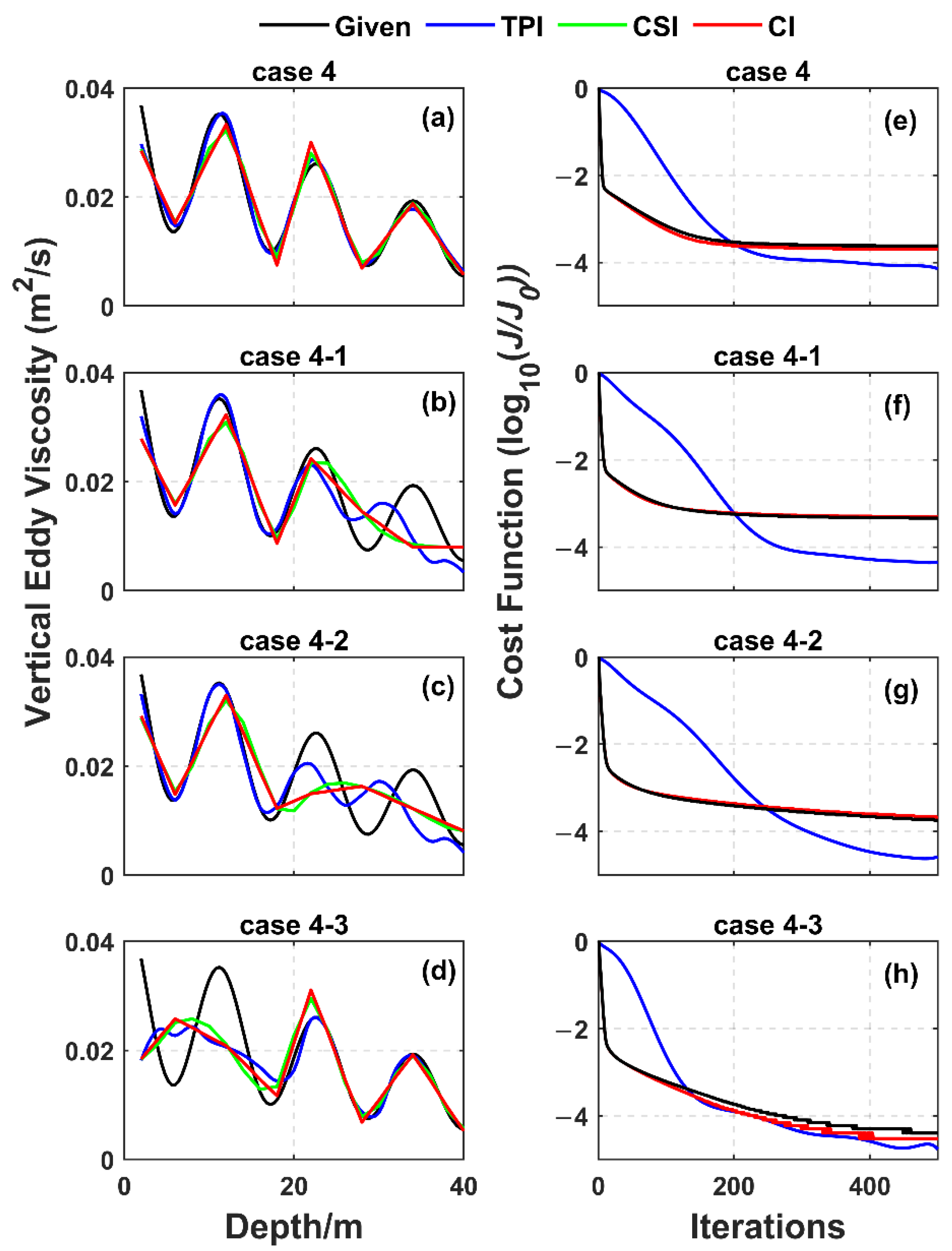
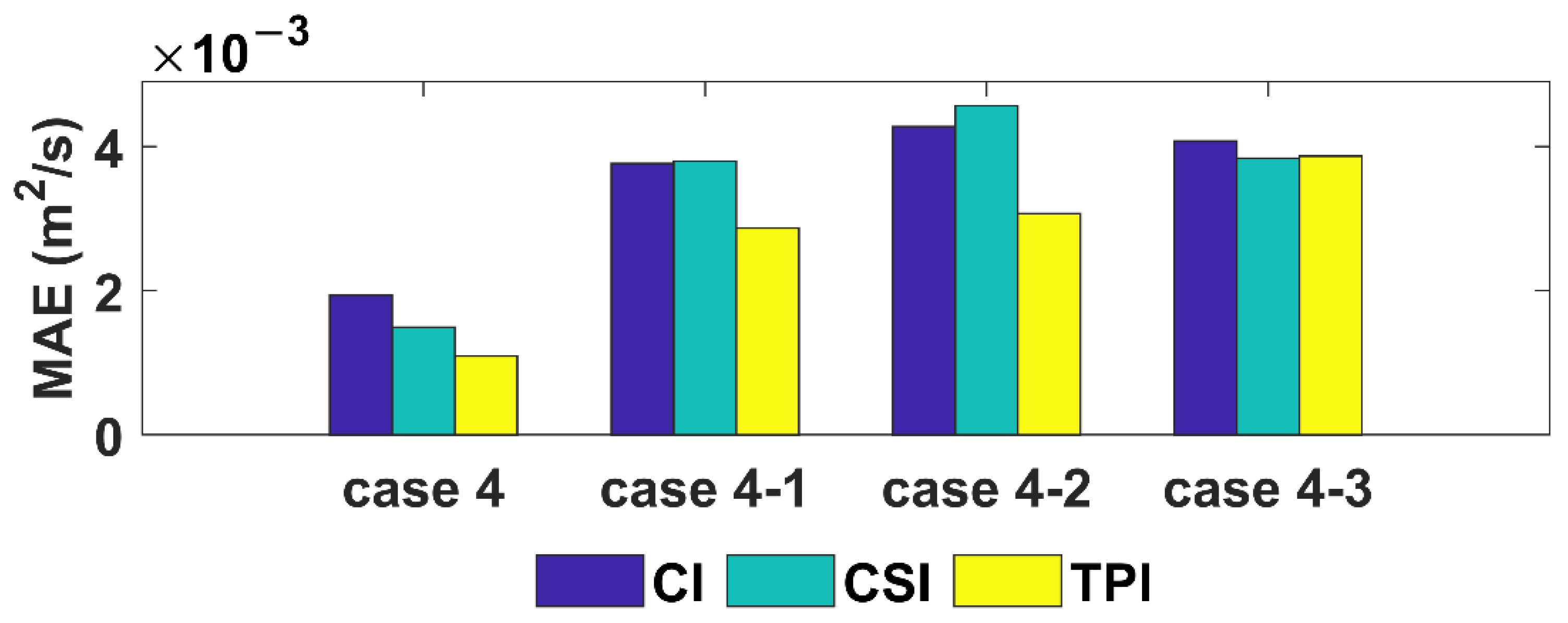
3.2. Group 1: Estimation of Given VEVCs

Since the distributions of VEVCs in the actual ocean cannot be completely observed, it was necessary to explore whether prescribed VEVCs could be handled by the model. The following four prescribed VEVC distributions were considered within this group and varied from simple to complex.

• Case 1: $\mathit{A}(\mathit{z})=\mathbf{0.045}(\mathbf{1}\mathbf{+}\mathbf{0.5}\mathbf{cos}(\frac{\mathbf{2}\mathit{\pi }\mathit{z}}{\mathbf{2}{\mathit{H}}_{\mathbf{0}}}))\mathbf{exp}(\frac{\mathbf{3}(\mathbf{\Delta }\mathit{Z}-\mathit{z})}{\mathbf{2}({\mathit{H}}_{\mathbf{0}}-\mathbf{\Delta }\mathit{Z})})\mathbf{,}$
• Case 2: $\mathit{A}(\mathit{z})=\mathbf{0.045}(\mathbf{1}\mathbf{+}\mathbf{0.5}\mathbf{cos}(\frac{\mathbf{6}\mathit{\pi }\mathit{z}}{\mathbf{2}{\mathit{H}}_{\mathbf{0}}}))\mathbf{exp}(\frac{\mathbf{3}(\mathbf{\Delta }\mathit{Z}-\mathit{z})}{\mathbf{2}({\mathit{H}}_{\mathbf{0}}-\mathbf{\Delta }\mathit{Z})})\mathbf{,}$
• Case 3: $\mathit{A}(\mathit{z})=\mathbf{0.045}(\mathbf{1}\mathbf{+}\mathbf{0.5}\mathbf{cos}(\frac{\mathbf{10}\mathit{\pi }\mathit{z}}{\mathbf{2}{\mathit{H}}_{\mathbf{0}}}))\mathbf{exp}(\frac{\mathbf{3}(\mathbf{\Delta }\mathit{Z}-\mathit{z})}{\mathbf{2}({\mathit{H}}_{\mathbf{0}}-\mathbf{\Delta }\mathit{Z})})\mathbf{,}$
• Case 4: $\mathit{A}(\mathit{z})=\mathbf{0.045}(\mathbf{1}\mathbf{+}\mathbf{0.5}\mathbf{cos}(\frac{\mathbf{14}\mathit{\pi }\mathit{z}}{\mathbf{2}{\mathit{H}}_{\mathbf{0}}}))\mathbf{exp}(\frac{\mathbf{3}(\mathbf{\Delta }\mathit{Z}-\mathit{z})}{\mathbf{2}({\mathit{H}}_{\mathbf{0}}-\mathbf{\Delta }\mathit{Z})})\mathbf{.}$

The distributions of the given VEVCs, the inverse distributions, and the normalized cost function are shown in Figure 1. The mean absolute errors (MAEs) between the given and the inverse values of the VEVCs in Group 1 are shown in Figure 2. As shown in Figure 1, the distribution of the given VEVC could be successfully inverted by all three interpolation schemes. However, since the VEVC inversion results produced by the CI scheme increased and decreased linearly, as opposed to the gentler oscillatory pattern of the given VEVC, the largest disagreement in the results occurred at the peaks and troughs. As shown in the variation of the normalized cost function, the estimated results using the TPI scheme were much better than those using the CI and CSI schemes. The cost functions of the CI and the CSI schemes eventually decreased by approximately 2–3 orders of magnitude in Cases 1–4, while those of the TPI scheme decreased by approximately 3–4 orders of magnitude. The MAEs between the given and inversed VEVCs proved that the results of the TPI scheme were in good agreement with the given distribution. This was most evident in Case 1.

The above results indicate that when the VEVC varied smoothly (Case 1), the given distribution could be successfully inverted by the three schemes, but when the VEVC varied abruptly, the inversion effect was better in the TPI scheme. Furthermore, the CI and CSI schemes required the consideration of a suitable selection of IPs, while the TPI scheme could ignore IP selection and thus reduce the workload. In summary, the Ekman layer model presented in this study could invert different VEVC distributions using different interpolation schemes. For any given distribution of the VEVCs, the inversion results of the TPI scheme varied the least and were the most similar to the given distributions.

3.3. Group 2: Effect of Missing Observations at Partial Depths

In Group 1, observations at all layers were used to restrict the ill-posedness of the inverse problem. However, field observations may not be spatially continuous or may not be available at all depths due to factors such as instrument failure. According to a study by Zhang et al. [25], the given eddy viscosity coefficients can be successfully inverted using only partial observations, and the Ekman model inversion is more sensitive to the upper-layer flow velocity. In this group, observations of partial layers were selected to explore the impact of missing data on the inversion schemes. The cases specifically included layers 1–10, 1–5, and 11–20, corresponding to Case 4-1, Case 4-2, and Case 4-3, respectively.

The given and inverted VEVCs for different observation layers and the normalized cost functions are shown in Figure 3. The MAEs in Group 2 are shown in Figure 4. In Case 4-1 and Case 4-2, the given distribution could be sufficiently inverted by all three schemes for the depths at which the observations existed. However, for the interval of missing observations between 20 and 40 m, the inversion results of the TPI scheme were a closer match to the given distribution compared with the other two schemes. Furthermore, in the interval of missing observations between 0 and 20 m, Case 4-3, the inversion results of all three schemes were poorly matched to the given distribution. After 300 iterations, the cost functions of the TPI schemes in both Case 4-1 and Case 4-2 were significantly lower than those of the other two schemes. However, in Case 4-3, there was no significant difference between the cost functions of the three schemes. This phenomenon was also observed in the MAEs between the inversion results and the given distribution (Figure 4), i.e., the optimization of the TPI scheme was apparent in Case 4-1 and Case 4-2 but less so in Case 4-3. These results indicate that the inverted results were more sensitive to the upper-level observations as opposed to the observations at the deeper layer, which is consistent with previous findings [25]. However, there was a difference between the results derived from partial observation only (Case 4-1 to Case 4-3) and the results using all observations (Case 4); the inverted VEVCs of this group were still acceptable, which suggests that the TPI scheme based on the present model can be adapted to accommodate missing observations from the ocean environment.

3.4. Group 3: Effect of the Boundary Layer Depth

The Ekman boundary layer depth (BLD) plays an important role in the formation of the Ekman currents. Yoshikawa and Endoh [24] tested the sensitivity of the VEVC to the selected BLDs. In this group, three different BLDs were designed, namely, Case 4-4, Case 4-5, and Case 4-6, which correspond to depths of 20 m, 50 m, and 80 m, respectively. The BLD is difficult to determine; hence, the BLD in this group refers to the model coverage depth.

The inversion results, given distributions, and the normalized cost function are shown in Figure 5. The MAEs of the inverted and given distributions in Group 3 are shown in Figure 6. In Cases 4-4 to 4-6, the given distributions were essentially inverted by all three schemes, but the inversion results of the TPI scheme were smoother. While the cost functions of the TPI scheme all decreased by four to five orders of magnitude, those of the other two schemes only decreased by three or four orders of magnitude. This indicates that the TPI scheme is better than others when different BLDs are selected. In every case, the MAE is the smallest when using the TPI scheme. In addition, the MAEs of Case 4 and Case 4-5 are smaller than those of the other two cases, indicating that an appropriate increase in the boundary layer thickness can help improve the inversion accuracy.

This experimental group demonstrated that the inversion results of a thick BLD were marginally superior to those of a thin BLD. In addition, the TPI scheme was more advantageous under these conditions.

3.5. Group 4: Effect of Noisy Data

In all the above experiments, the observed currents were directly calculated by the forward model, and the wind velocities were provided. However, in practice, observational current and wind velocity data may contain errors, which might adversely affect the inversion results. Zhang and Lu [31] argued that the average discrepancy between the inverse results and the observed values increased anomalously as the error increased. In this section, random errors were introduced to the “observations” presented in Cases 4-7, 4-8, 4-9, and 4-10. A certain percentage of Gaussian white noise was added to the observation of currents $u\left(i,j\right)$ and $v\left(i,j\right)$ and wind velocities $u_a\left(i,j\right)$ to simulate actual observation error. The maximum percentages of random errors were 2%, 5%, 10%, and 15%.

The inverse and given distributions and the normalized cost function are shown in Figure 7. The MAEs with different noises in Group 4 are shown in Figure 8. The TPI scheme had a better overall inversion performance in all four cases, while the inversion results of the other two schemes differed substantially from the given distribution due to the abrupt variations in the VEVCs. As the observation errors increased, the magnitude of the cost function was gradually reduced. For example, the cost function for Case 4-7 decreased by 2 to 3 orders of magnitude, while the cost function for Case 4-10 decreased by less than 1 order of magnitude. As seen in Figure 8, the MAEs of the three schemes only increased slightly as the observation errors increased, and the MAE of the TPI scheme was obviously smaller than that of the CI and CSI schemes. The above results suggest that the observation errors have an impact on the inversion results, but the TPI scheme can enhance the stability of the model performance and estimate the VEVC well.

Due to the rapid development of ocean current measurement techniques, errors in velocity measurements of the acoustic doppler current profiler can be adequately controlled [32,33], especially after manual selection and quality screening. Hence, the TPI scheme is believed to be able to withstand a certain degree of noise within data.

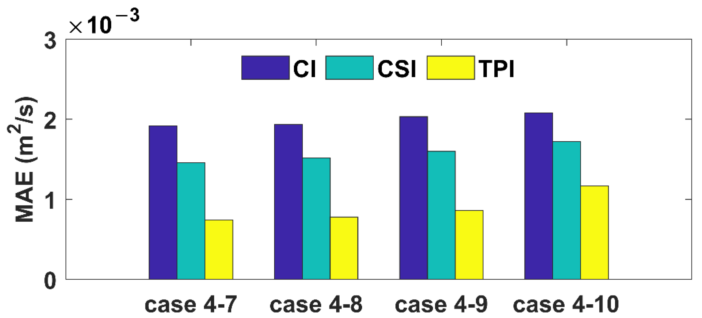
3.6. Group 5: Effect of Wind Stress Drag Coefficient Optimization

The wind stress drag coefficients in the above experiments were all fixed as constants. However, in the actual environment, the drag coefficients are usually variable and strongly correlated with wind speed. In this experiment, the following three initial distributions of drag coefficients were selected in order to investigate the influence of different wind stress drag coefficients on the different inversion schemes. As the model cycled through each iteration, the drag coefficients were optimized dynamically rather than remaining static. The initial wind stress drag coefficient was set to 1.2 × 10⁻³.

• Case 4-11: ${\mathit{C}}_{\mathit{d}}(\mathit{t})=(0.8\mathbf{+}0.065\mathbf{\times }{\mathit{U}}_{10})\mathbf{\times }{10}^{-3}$
• Case 4-12: ${\mathit{C}}_{\mathit{d}}(\mathit{t})=(0.61\mathbf{+}0.063\mathbf{\times }{\mathit{U}}_{10})\mathbf{\times }{10}^{-3}$
• Case 4-13: ${\mathit{C}}_{\mathit{d}}(\mathit{t})=0.0012$

The inverse and given distributions of the VEVCs, as well as the normalized cost function, are shown in Figure 9. The MAEs in Group 5 are shown in Figure 10. When different wind stress drag coefficient distributions were chosen, the given VEVC distributions could still be inverted by all three interpolation schemes. In Cases 4-11 and 4-12, the cost functions for all three schemes decreased by approximately two orders of magnitude. In Case 4-13, the cost function of the CI and CSI schemes decreased by approximately three orders of magnitude, while the cost function of the TPI scheme decreased by approximately 4 orders of magnitude. The cost function of Case 4-13 was lower than those of Cases 4-11 and 4-12. These results demonstrate that optimizing the wind stress drag coefficients yielded more notable improvements in inversion model performance than could be otherwise obtained by setting different distributions of the initial wind stress drag coefficient. The MAEs between the inversion results and the given distributions also support this point. The MAEs calculated using the TPI scheme were lower in Cases 4-11, 4-12, and 4-13 than in Case 4.

In summary, the accuracy of the inversion results could be improved by iteratively optimizing the time-varying wind stress drag coefficient. Compared with the inversion using the CSI and CI schemes, the inversion using the TPI scheme was more effective.

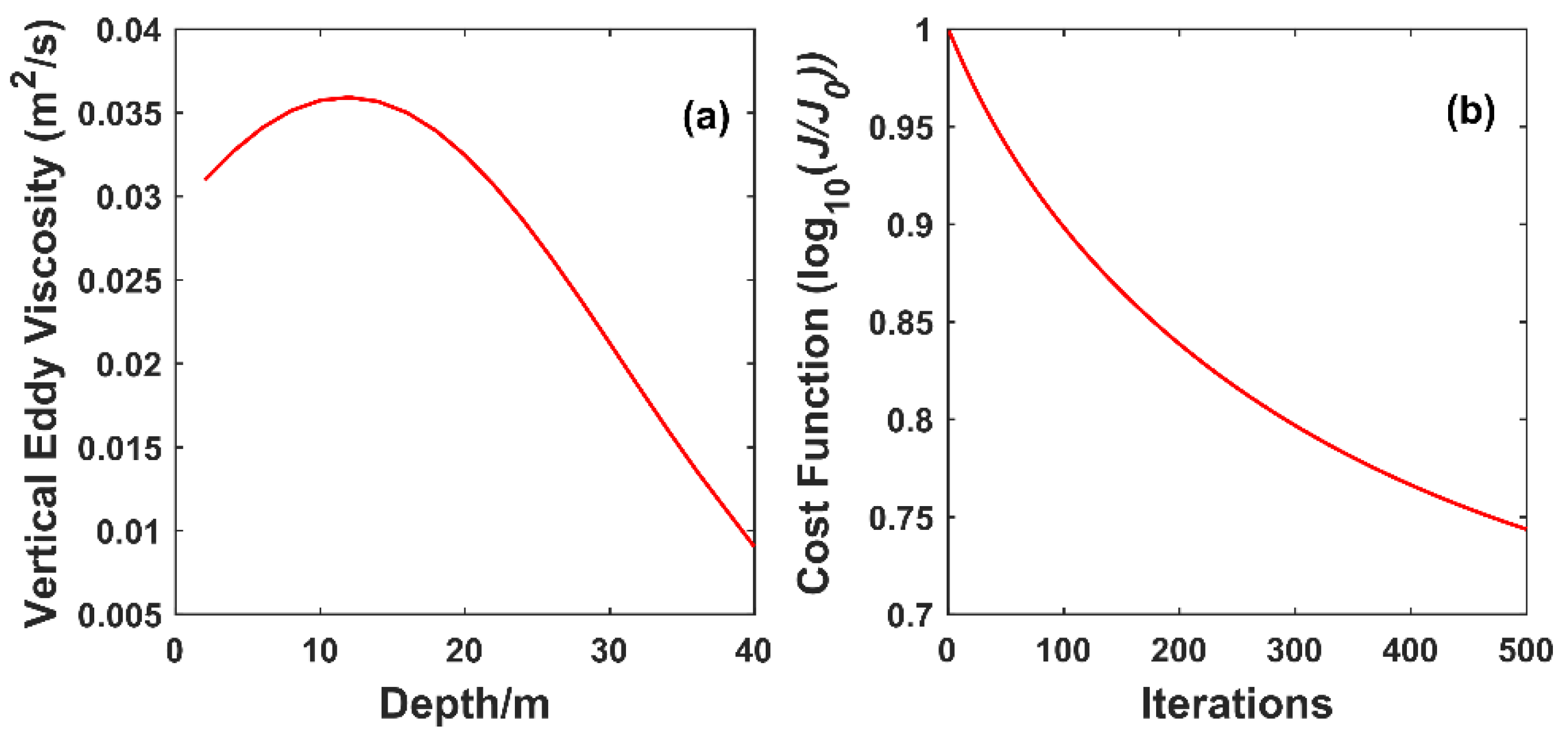
4. Practical Experimentation and Results

4.1. Data and Experimental Design

In the previous experiments, the inversion performance of the TPI scheme was verified in several ways. This demonstrates that both the inversion stability and precision of the TPI scheme were superior to the other two schemes based on the original model. However, the capability of the TPI scheme still needed to be verified with in situ experimentation. Observations from Yellow Sea station buoy 17, which predominately contains wind speed and current data, were used to achieve this. Current velocity data were measured between depths of 3 and 41 m, with a spatial resolution of 2 m and a temporal resolution of 10 min. Wind speed was measured 4 m above the sea surface at a temporal resolution of 10 min. Wind speed 10 m above the surface (U₁₀) was calculated using the equation proposed by Large et al. and the method outlined by Zedler et al. [34,35].

In this section, the wind stress drag coefficient was set as a function of time, with an initial C_d(t) value of 0.0012. The initial VEVC value, A(z), was set to 0.008 m²/s. The initial conditions were obtained by linearly interpolating the currents observed by Yellow Sea station buoy 17 at 21:20 on 16 November 2016. The model was driven by the wind speed U₁₀, which was calculated from the observed wind speed. The time step used in the model was 0.5 h, and the vertical resolution was 2 m. In this set of experiments, only the observations of the first 14 layers (between the depths of 3 and 29 m) were used in the model due to the large proportion of missing measurements. The interval between 16 November at 21:00 and 17 November at 21:00 was regarded as the cold start. The model was forward integrated over the following 9 days to generate the simulated Ekman currents, and the adjoint variables were then calculated by backward integrating the adjoint model. The VEVC was optimized and inverted by the TPI scheme, as described in Section 2. The Coriolis parameter was calculated on the basis of the buoy’s latitude, and the other settings were the same as those in the previous twin experiments.

4.2. Results

The reliability of the TPI scheme was demonstrated by the inversion results and by how the normalized cost function decreased with increased iterations, as shown in Figure 11. The cost function decreased continuously from 1 to approximately 0.75, which indicated that applying the TPI scheme in the model effectively reduced the difference between observations and simulated Ekman current velocities. Panel (a) in Figure 11 shows an initial and marginal increase in the VEVC before it transitioned to a decreasing trend at depths within 40 m. The range of the inverse VEVC was 0.0091–0.0359 m²/s, which is more in line with previous studies [21].

The plots in Figure 12 show the simulated and observed currents at depths from 3 to 29 m. The amplitudes and phases of the simulated and observed currents were in good agreement overall, although there were brief intervals where they did not perfectly align. In addition, the simulated results in the U direction were in particularly good agreement with the observed values. This suggests that the combination of the TPI scheme and the adjoint method can produce reasonable Ekman currents, which is beneficial in terms of using and improving observational data. In summary, field observations were used to verify the feasibility of the TPI scheme and demonstrate the stability of the inversion results.

In previous studies, the VEVC has usually been set as a constant or a profile estimated from a turbulence model. Taking this into account, the VEVC, set as a constant (0.006 m²/s), and the VEVC, estimated by a dual-range turbulence closure model, were selected as comparisons with the results in this manuscript [21,36]. Then the MAEs between inverted current velocities and observations were calculated separately in different cases. The present scheme corresponded to Case 5, and the first two cases with selected VEVCs corresponded to Case 6 and Case 7, respectively. The MAEs between the inverted current velocities and the observed velocities for each layer from 1 to 14 are shown in Figure 13. It can be seen that the MAEs in Case 5 were both significantly smaller than those in Case 6 and Case 7, which indicates that the model and TPI scheme will contribute to the development of studies related to the eddy viscosity coefficient.

5. Conclusions

Conditions in the ocean vary temporally; thus, parameters defined by dynamic ocean processes should also be temporally variable. This work presented a modified Ekman model, in which the VEVC was inverted using a TPI scheme based on the adjoint assimilation technique. Five sets of twin experiments were conducted to examine the effects of various factors on the inversion results obtained with this scheme. These factors included the VEVC distribution, missing data, BLD, wind stress drag coefficient distribution, and noisy observational data. The main conclusions are as follows.

The ability of the three interpolation schemes to estimate different prescribed distributions of the VEVCs was compared in Group 1. The results demonstrated that different distributions could be inverted successfully using the Ekman model and that the TPI scheme had the best performance among the three interpolation schemes. Group 2 explored the effect of missing data from different observational layers. The results showed that the models were more sensitive to observations from the upper layers and that the inversion results of the TPI scheme were more accurate. Group 3 studied the response of the model to the BLD. The results revealed that the TPI scheme could sufficiently accommodate the effect of different BLDs. The effect of noisy observational data was addressed in Group 4. The inversion results converged with the given VEVC distributions despite the noise in the data. This indicates that the TPI scheme can account for noisy data to some degree. Group 5 examined the effect of the distribution of drag coefficients for VEVCs. The results illustrated that the inversion accuracy could be enhanced by selecting the time-varying distribution of wind stress drag coefficients and that the inversion results of the TPI scheme were more precise under those conditions.

The TPI scheme was further validated by practical experimentation. The vertical profile of the VEVC was successfully inverted by assimilating current and wind speed observations from buoy 17 in the Yellow Sea into the model. The result of this experiment was consistent with previous findings. Additionally, the simulated and observed currents were closely aligned.

In this study, the typical Ekman model was modified so that the VEVC was not constant, and a vertical profile was obtained by assimilating in situ measurements. The VEVC estimation method used in this paper was based on the inverse problem and parameter estimation theory combined with the TPI scheme, which is an improvement over the conventional parameter estimation method. This research furthers our understanding of the Ekman layer model and offers an alternative scheme for determining the VEVC. Future work will concentrate on the problem of parameter estimation under extreme wind conditions and discuss the spatial distribution and temporal variation of the VEVC in the actual ocean when subjected to strong winds.

References

1. Zhang, Y.; Tian, J.; Xie, L. Estimation of eddy viscosity on the South China Sea shelf with adjoint assimilation method. Acta Oceanol. Sin. 2009, 28, 9–16. [Google Scholar]
2. Levermore, C.D.; Sammartino, M. A shallow water model with eddy viscosity for basins with varying bottom topography. Nonlinearity 2001, 14, 1493–1515. [Google Scholar] [CrossRef]
3. Pedlosky, J. Geophysical Fluid Dynamics; Springer: Berlin/Heidelberg, Germany, 1987; Volume 710. [Google Scholar]
4. Yoshikawa, Y.; Matsuno, T.; Wagawa, T.; Hasegawa, T.; Nishiuchi, K.; Okamura, K.; Yoshimura, H.; Morii, Y. Tidal and low-frequency currents along the CK Line (31deg 45min N) over the East China Sea shelf. Cont. Shelf Res. 2012, 50–51, 41–53. [Google Scholar] [CrossRef]
5. Davies, A.M.; Xing, J. The influence of eddy viscosity parameterization and turbulence energy closure scheme upon the coupling of tidal and wind induced currents. Estuar. Coast. Shelf Sci. 2001, 53, 415–436. [Google Scholar] [CrossRef]
6. Lenn, Y.D.; Chereskin, T.K. Observations of Ekman currents in the Southern Ocean. J. Phys. Oceanogr. 2009, 39, 768–779. [Google Scholar] [CrossRef] [Green Version]
7. Zhao, R.; Vallis, G. Parameterizing mesoscale eddies with residual and Eulerian schemes, and a comparison with eddy-permitting models. Ocean Model. 2008, 23, 1–12. [Google Scholar] [CrossRef]
8. Song, J.B.; Huang, Y.S. An approximate solution of wave-modified Ekman current for gradually varying eddy viscosity. Deep. Res. Part I Oceanogr. Res. Pap. 2011, 58, 668–676. [Google Scholar] [CrossRef]
9. Song, J.B.; Xu, J.L. Wave-modified Ekman current solutions for the vertical eddy viscosity formulated by K-Profile Parameterization scheme. Deep. Res. Part I Oceanogr. Res. Pap. 2013, 80, 58–65. [Google Scholar] [CrossRef]
10. Price, J.F.; Weller, R.A.; Schudlich, R.R. Wind-Driven Ocean currents and Ekman transport. Science 1987, 238, 1534–1538. [Google Scholar] [CrossRef] [Green Version]
11. Chereskin, T.K. Direct evidence for an Ekman balance in the California Current. J. Geophys. Res. 1995, 100, 18261–18269. [Google Scholar] [CrossRef]
12. Elipot, S.; Gille, S.T. Ekman layers in the Southern Ocean: Spectral models and observations, vertical viscosity and boundary layer depth. Ocean Sci. 2009, 5, 115–139. [Google Scholar] [CrossRef] [Green Version]
13. Polton, J.A.; Lenn, Y.D.; Elipot, S.; Chereskin, T.K.; Sprintall, J. Can drake passage observations match ekman’s classic theory. J. Phys. Oceanogr. 2013, 43, 1733–1740. [Google Scholar] [CrossRef] [Green Version]
14. Roach, C.J.; Phillips, H.E.; Bindoff, N.L.; Rintoul, S.R. Detecting and characterizing Ekman currents in the Southern Ocean. J. Phys. Oceanogr. 2015, 45, 1205–1223. [Google Scholar] [CrossRef]
15. Ferreira, V.G.; Mangiavacchi, N.; Tomé, M.F.; Castelo, A.; Cuminato, J.A.; McKee, S. Numerical simulation of turbulent free surface flow with two-equation k-ε eddy-viscosity models. Int. J. Numer. Methods Fluids 2004, 44, 347–375. [Google Scholar] [CrossRef]
16. Pacanowski, R.; Philander, S. Parameterization of Vertical Mixing in Numerical Models of Tropical Oceans. J. Phys. Oceanogr.-J. PHYS Ocean. 1981, 11, 1443–1451. [Google Scholar] [CrossRef]
17. Mellor, G.L. USERS GUIDE for OCEAN MODEL. Ocean Model. 2004, 8544, 0710. [Google Scholar]
18. Odier, P.; Chen, J.; Rivera, M.K.; Ecke, R.E. Fluid mixing in stratified gravity currents: The prandtl mixing length. Phys. Rev. Lett. 2009, 102, 134504. [Google Scholar] [CrossRef] [Green Version]
19. Wang, Y.; Qiao, F.; Fang, G.; Wei, Z. Application of wave-induced vertical mixing to the K profile parameterization scheme. J. Geophys. Res. Ocean. 2010, 115, 1–12. [Google Scholar] [CrossRef]
20. Zhang, J.; Lu, X. Inversion of three-dimensional tidal currents in marginal seas by assimilating satellite altimetry. Comput. Methods Appl. Mech. Eng. 2010, 199, 3125–3136. [Google Scholar] [CrossRef]
21. Yu, L.; O’Brien, J.J. Variational Estimation of the Wind Stress Drag Coefficient and the Oceanic Eddy Viscosity Profile. J. Phys. Oceanogr. 1991, 21, 709–719. [Google Scholar] [CrossRef] [Green Version]
22. Cao, A.; Chen, H.; Fan, W.; He, H.; Song, J.-B.; Zhang, J.-C. Estimation of Eddy Viscosity Profile in the Bottom Ekman Boundary Layer. J. Atmos. Ocean. Technol. 2017, 34, 2163–2175. [Google Scholar] [CrossRef]
23. Yoshikawa, Y.; Endoh, T.; Matsuno, T.; Wagawa, T.; Tsutsumi, E.; Yoshimura, H.; Morii, Y. Turbulent bottom Ekman boundary layer measured over a continental shelf. Geophys. Res. Lett. 2010, 37, 1–5. [Google Scholar] [CrossRef] [Green Version]
24. Yoshikawa, Y.; Endoh, T. Estimating the eddy viscosity profile from velocity spirals in the Ekman boundary layer. J. Atmos. Ocean. Technol. 2015, 32, 793–804. [Google Scholar] [CrossRef] [Green Version]
25. Zhang, J.; Li, G.; Yi, J.; Gao, Y.; Cao, A. A method on estimating time-varying vertical eddy viscosity for an ekman layer model with data assimilation. J. Atmos. Ocean. Technol. 2019, 36, 1789–1812. [Google Scholar] [CrossRef] [Green Version]
26. Chen, H.; Cao, A.; Zhang, J.; Miao, C.; Lv, X. Estimation of spatially varying open boundary conditions for a numerical internal tidal model with adjoint method. Math. Comput. Simul. 2014, 97, 14–38. [Google Scholar] [CrossRef]
27. Jiang, D.; Chen, H.; Jin, G.; Lv, X. Estimating smoothly varying open boundary conditions for a 3D internal tidal model with an improved independent point scheme. J. Atmos. Ocean. Technol. 2018, 35, 1299–1311. [Google Scholar] [CrossRef]
28. Jin, G.; Pan, H.; Zhang, Q.; Lv, X.; Zhao, W.; Gao, Y. Determination of harmonic parameters with temporal variations: An enhanced harmonic analysis algorithm and application to internal tidal currents in the South China Sea. J. Atmos. Ocean. Technol. 2018, 35, 1375–1398. [Google Scholar] [CrossRef]
29. Nie, Y.; Wang, Y.; Lv, X. Acquiring the arctic-scale spatial distribution of snow depth based on AMSR-E snow depth product. J. Atmos. Ocean. Technol. 2019, 36, 1957–1965. [Google Scholar] [CrossRef]
30. Wu, X.; Xu, M.; Gao, Y.; Lv, X. A scheme for estimating time-varying wind stress drag coefficient in the ekman model with adjoint assimilation. J. Mar. Sci. Eng. 2021, 9, 1220. [Google Scholar] [CrossRef]
31. Zhang, J.; Lu, X. Parameter estimation for a three-dimensional numerical barotropic tidal model with adjoint method. Int. J. Numer. Methods Fluids 2008, 57, 47–92. [Google Scholar] [CrossRef]
32. De Serio, F.; Mossa, M. Analysis of mean velocity and turbulence measurements with ADCPs. Adv. Water Resour. 2015, 81, 172–185. [Google Scholar] [CrossRef]
33. Nystrom, E.A.; Rehmann, C.R.; Oberg, K.A. Evaluation of Mean Velocity and Turbulence Measurements with ADCPs. J. Hydraul. Eng. 2007, 133, 1310–1318. [Google Scholar] [CrossRef] [Green Version]
34. Zedler, S.E.; Dickey, T.D.; Doney, S.C.; Price, J.F.; Yu, X.; Mellor, G.L. Analyses and simulations of the upper ocean’s response to Hurricane Felix at the Bermuda Testbed Mooring site: 13-23 August 1995. J. Geophys. Res. Oceans 2002, 107, 13–23. [Google Scholar] [CrossRef] [Green Version]
35. Large, W.G.; Pond, S. Open Ocean Momentum Flux Measurements in Moderate to Strong Winds. J. Phys. Oceanogr. 1981, 11, 324–336. [Google Scholar] [CrossRef] [Green Version]
36. Lee, J.C.; Jung, K.T. Application of eddy viscosity closure models for the M2 tide and tidal currents in the Yellow Sea and the East China Sea. Cont. Shelf Res. 1999, 19, 445–475. [Google Scholar] [CrossRef]
Figure 1. On the left are the prescribed and inverted VEVCs obtained by different interpolation schemes in the model. Panels (ad) correspond to Cases 1–4, respectively. On the right are the variation curves of the cost functions in Group 1. Panels (eh) correspond to Cases 1–4, respectively.
Jmse 10 01165 g001
Figure 2. The MAEs between the prescribed and inverted VEVCs with three schemes in Cases 1–4.
Jmse 10 01165 g002
Figure 3. The prescribed and inversion distributions of the VEVCs after using different observation depths on the left. (ad) correspond to Cases 4, 4-1, 4-2, and 4-3, respectively. On the right are the cost functions of the three schemes in Group 2. (eh) correspond to Cases 4, 4-1, 4-2, and Case 4-3, respectively.
Jmse 10 01165 g003
Figure 4. The MAEs between the given and inverted VEVCs with three schemes in Cases 4, 4-1, 4-2, and 4-3.
Jmse 10 01165 g004
Figure 5. On the left are the prescribed and inversion distributions of the VEVCs after using different BLDs. Panels (ad) correspond to Cases 4-4, 4-5, 4-6, and 4, respectively. On the right are the cost functions of the three schemes in Group 3. Panels (eh) correspond to Cases 4-4, 4-5, 4-6, and 4, respectively.
Jmse 10 01165 g005
Figure 6. The MAEs between the given and inverted VEVCs with different BLDs in Cases 4-3, 4-5, 4-6, and 4.
Jmse 10 01165 g006
Figure 7. On the left are the prescribed and inverted distributions of the VEVCs after adding 2% (a), 5% (b), 10% (c), and 15% (d) errors, respectively. On the right are the cost functions of the three schemes in Group 4. Panels (ad) and (eh) correspond to Cases 4-7, 4-8, 4-9, and 4-10, respectively.
Jmse 10 01165 g007
Figure 8. The MAEs between the given and inverted VEVCs with the assimilation steps after adding 2%, 5%, 10%, and 15% errors.
Jmse 10 01165 g008
Figure 9. On the left are the prescribed and inverted distributions of the VEVCs after using different distributions of wind stress drag coefficients. Panels (ac) correspond to Cases 4-11, 4-12, and 4-13, respectively. On the right are the cost functions using the three schemes in Group 5. Panels (df) correspond to Cases 4-11, 4-12, and 4-13, respectively.
Jmse 10 01165 g009
Figure 10. The MAEs between the prescribed and inverted VEVCs after using different distributions of wind stress drag coefficients to Cases 4-11, 4-12, 4-13, and 4.
Jmse 10 01165 g010
Figure 11. The left panel (a) shows the inverted distributions of the VEVC in the practical experiment. The right panel (b) is the cost function in the practical experiment.
Jmse 10 01165 g011
Figure 12. Temporal distribution of observed and inverted current velocities to the east (left) and north (right). The uppermost plots depict current velocities at a depth of 3 m with subsequent plots showing velocities at 2 m increments to a maximum depth of 29 m at the bottom. U and V denote the inverse current velocities in the zonal and meridional directions, respectively.
Jmse 10 01165 g012
Figure 13. The MAEs between inverted currents and observed currents in Cases 5, 6, and 7. Subplots (a,b) correspond to the horizontal velocity components U and V, respectively.
Jmse 10 01165 g013