Underwater Electromagnetic Guidance Based on the Magnetic Dipole Model Applied in AUV Terminal Docking

Abstract

To address the poor effect of optical/visual guidance used in AUV terminal docking with strong background light and turbid water quality, an underwater electromagnetic guidance method based on the magnetic dipole model is proposed in this paper. According to the magnetic dipole model, the electromagnetic field of 1 kHz frequency generated by the coil in the range of terminal docking is the near field, where the position can be figured out through the amplitude and phase information of three orthogonal magnetic field intensity vectors. A triaxial-coil magnetometer with three orthogonal coils and a method for extracting the amplitude and phase information of the induced voltage are presented in this paper. According to Faraday’s law, the amplitude and phase information of the induced voltage of a triaxial-coil magnetometer replace the information of magnetic field intensity in relation to positioning. The underwater positioning results show that the average positioning error within 6 m can reach the centimeter level. Five underwater terminal docking tasks were carried out, and four of them were successfully completed, which verified the feasibility of the proposed method.

1. Introduction

Docking systems that use an underwater autonomous vehicle (AUV) and docking station (DS) are commonly used for observing the ocean [1,2,3,4]. AUV navigation is an important technology to ensure that AUVs can smoothly enter the DS [5,6]. AUV navigation is mainly divided into two stages: remote homing when the AUV is far away from the DS and terminal docking when the AUV is close to the DS [7,8,9]. Generally, in remote homing, the AUV is more than 20 m away from the DS, while in terminal docking, the distance between the AUV and the DS station is approximately 5–20 m. The required AUV navigation accuracy and real-time positioning performance are not highly required since the AUV is far from the DS during remote homing. Therefore, acoustic sensors are usually used for navigation, especially the ultra-short baseline (USBL) acoustic positioning device [10,11]. When the AUV starts terminal docking, it needs high navigation accuracy and a high frequency of positioning so that optical navigation [12], visual navigation [13], and electromagnetic navigation [8] can be adopted. However, optical and visual methods can only be applied in water with high quality and a simple background. Therefore, the electromagnetic method has been proposed.

Feezor et al. first put forward the electromagnetic method for docking navigation with an effective range of 25–30 m [8]. In this method, three large coils are installed on the underwater DS, and three small coils with mutually perpendicular axes are installed on the AUV. However, there are three large transmitting coils in the electromagnetic guidance system, which makes it difficult to install in practical applications and takes up space for other equipment. In addition, the scheme cannot realize the positioning function. Vandavasi et al. developed an electromagnetic navigation system for AUV docking based on the bionic concept of migratory birds and conducted modeling and simulation with electromagnetic field finite element analysis (FEA) tools [14]. The system includes a coil and a magnetometer installed in the AUV. According to the electromagnetic field spectrum obtained by the FEA software, the system can calculate the bear angle for docking. However, this scheme cannot realize the positioning function. The electromagnetic guidance method was verified on the surface of water in a pool test with an effective range of 7 m. The trouble is that the electromagnetic field distribution through FEA should be obtained in advance, which greatly reduces the universality of the system. Peng et al. proposed a low-cost electromagnetic guidance system, which includes a large square magnetic beacon and a triaxial-coil receiver with an effective range of 20 m [15,16]. The transmitting coil generates a 1 kHz electromagnetic field, and the triaxial-coil magnetometer installed in the head of the AUV senses the magnetic field intensity. The magnetic field information is used to determine the angle between the AUV axis and magnetic line in order to guide the AUV. However, the transmitting coil is too large to generate enough of a magnetic moment, which means it is difficult to install it in the DS. Furthermore, the position of AUV relative to the DS also cannot be obtained by this method. In the scheme, a docking task was carried out on the surface of water in a pool experiment to verify the electromagnetic guidance with an effective range of approximately 20 m. Based on the attenuation law of electromagnetic waves in water, Daegel Park et al. put forward a method of underwater positioning through the received signal strength (RSS) [17,18]. The system includes four electromagnetic wave signal transmitters and an electromagnetic wave intensity analyzer. The four electromagnetic wave transmitters generate identifiable electromagnetic signals. According to the attenuation relationship between the RSS and the distance, the position of the receiver can be calculated. This method was verified with an ROV in an underwater pool test with an effective range of approximately 6 m. Due to the high frequency of the electromagnetic waves used, the attenuation of electromagnetic waves in water (especially in seawater) is large, and thus the effective range is greatly shortened. To realize the application of the method, four electromagnetic wave transmitters should be installed near the DS, which is difficult to realize in practical docking applications. Compared with the above three schemes, the transmitters and receiver are relatively expensive equipment.

In this paper, an electromagnetic guidance method with a positioning function based on the magnetic dipole model is developed. A triaxial-coil magnetometer detected the changing 1 kHz-frequency magnetic field intensity generated by the transmitting coil as induced voltage. A positioning method based on the amplitude and relative phase of the induced voltage is proposed. Then, the positioning data are used to guide the AUV in terminal docking. The rest of this paper is organized as follows: Section 2 introduces the electromagnetic field distribution in the terminal docking area based on the magnetic dipole model. The design of a triaxial-coil magnetometer and a method for extracting the amplitude and phase information of the induced voltage are introduced in detail in Section 3. Section 4 explains the positioning method based on the induced voltage information of the triaxial-coil magnetometer. The AUV terminal docking guidance method according to the positioning data of the electromagnetic guidance system is also explained in this section. The configuration of the electromagnetic guidance system is introduced in Section 5. The results of positioning and AUV terminal docking experiments are discussed in Section 6. The electromagnetic guidance method is compared with the optical/visual guidance and the electromagnetic guidance method proposed by other institutions in Section 7. Finally, the last section presents the conclusions of this paper.

2. The Analysis of Electromagnetic Field Distribution in the Terminal Docking Area

An electromagnetic field can be generated when an AC current passes through the transmitting coil. The characteristics of electromagnetic field distribution will be analyzed in this part to find a method of obtaining the position information.

2.1. Magnetic Dipole Model

In AUV terminal docking guidance, the distance between the AUV and the center of the transmitting coil is much larger than the width and diameter of the coil itself, so the N-turn transmitting coil is approximately regarded as a magnetic dipole at the center of the central axis of the transmitting coil. We assume that the expression of the AC current flowing through the transmitting coil is:

$$i(t)=I\cos \omega t=\mathrm{Re}(\dot{I})=\mathrm{Re}(I{e}^{j\omega t}),$$

(1)

where $\omega$ and $I$ denote the angular frequency and amplitude of the AC current. The current is expressed in the form of a complex vector $\dot{I}$. For convenience, the time-varying quantities are expressed by complex vectors in subsequent articles. If the area of the magnetic dipole is $S$, then the magnetic moment $\dot{M}$ of the magnetic dipole is

$$\dot{M}=N\dot{I}S$$

(2)

The spherical coordinate $o-r\varphi \theta$ of the transmitting coil and the fixed coordinate in AUV terminal docking guidance are established as shown in Figure 1.

The dielectric constant, permeability, and conductivity of the medium near the coil are $\epsilon ,\mu ,\gamma$, respectively. The magnetic vector potential of any point $P$ in the spherical coordinate is

$$\dot{\mathit{A}}=\frac{\mu \dot{M}\sin \theta e^{-jkr}(1+jkr)}{4\pi r^2}{\mathit{e}}_{\varphi }$$

(3)

Hence, the magnetic field intensity vector $\dot{\mathit{H}}$ of this point is:

$$\dot{\mathit{H}}=\frac{1}{\mu }\nabla \times \dot{\mathit{A}}=\frac{\dot{M}}{2\pi }(\frac{1}{r^3}+\frac{jk}{r^2})\cos \theta e^{-jkr}{\mathit{e}}_r+\frac{\dot{M}}{4\pi }(\frac{1}{r^3}+\frac{jk}{r^2}-\frac{k^2}{r})\sin \theta e^{-jkr}{\mathit{e}}_{\theta },$$

(4)

where $k$ denotes the propagation constant of the electromagnetic wave. The propagation constant $k$ is equal to $\alpha -j\beta$, where $\alpha$ and $\beta$ denote the phase constant and attenuation constant, respectively. The expression of $\alpha$ and $\beta$ can be given as:

$$\begin{array}{l}\alpha =\omega \sqrt{\frac{\mu \epsilon }{2}[\sqrt{1+{(\frac{\gamma }{\omega \epsilon })}^2}+1]}\\ \beta =\omega \sqrt{\frac{\mu \epsilon }{2}[\sqrt{1+{(\frac{\gamma }{\omega \epsilon })}^2}-1]}\end{array}$$

(5)

The wavelength of the electromagnetic wave is related to the phase constant:

$$\lambda =\frac{2\pi }{\alpha }$$

(6)

If the distance $r$ between test point P and the center of the magnetic dipole satisfies the condition that $r<<\lambda$, the magnetic field intensity vector at point P is further simplified as:

$$\dot{\mathit{H}}=\frac{1}{\mu }\nabla \times \dot{\mathit{A}}=\frac{\dot{M}}{2\pi }\cos \theta {\mathit{e}}_r+\frac{\dot{M}}{4\pi }\sin \theta {\mathit{e}}_{\theta },$$

(7)

This is the near field, where the amplitude of the changing magnetic field intensity is very similar to that in the static field. There is no imaginary part in the expression of magnetic field intensity, which means that the phase of the magnetic field in both ${\mathit{e}}_r$ and ${\mathit{e}}_{\theta }$ directions is in-phase or anti-phase with the current passing through the transmitting coil. According to the transformation from spherical coordinates to rectangular coordinates in Figure 1, the magnetic field intensity of point P in fixed coordinates is:

$$\dot{\mathit{H}}=\frac{\dot{M}}{4\pi r^3}[(2{\cos }^2\theta -{\sin }^2\theta ){\mathit{e}}_x-3\sin \theta \cos \theta \cos \varphi {\mathit{e}}_y-3\sin \theta \cos \theta \sin \varphi {\mathit{e}}_z],$$

(8)

It can be seen that the magnetic field intensity in the near field is only related to the magnetic moment and position, which is independent of the conductivity, permeability, and dielectric constant of the medium. The permeability and dielectric constant are the same in air, freshwater, and seawater, where only the conductivity is different. If the frequency is 100 Hz, the wavelength in freshwater can reach 3162 m, and in seawater can reach 158 m. If the frequency of the electromagnetic wave increases to 1 kHz, the electromagnetic wavelength in freshwater is 1000 m, but that in seawater is reduced to 50 m. If the frequency is further increased, the wavelength of the electromagnetic wave will be shorter, and the distance that can meet the conditions of the near field will be shorter, which means that the electromagnetic guidance range will be shorter. Therefore, the 1 kHz low-frequency electromagnetic field is utilized in this paper.

2.2. Positioning Method

${\dot{\mathit{H}}}_x,{\dot{\mathit{H}}}_y,{\dot{\mathit{H}}}_z$ denote the magnetic field vector in three directions at point P in the near field excited by the transmitting coil in fixed coordinates. The complex vectors ${\dot{H}}_x,{\dot{H}}_y,{\dot{H}}_z$ are the modules of ${\dot{\mathit{H}}}_x,{\dot{\mathit{H}}}_y,{\dot{\mathit{H}}}_z$, respectively. In order to facilitate the subsequent judgement of whether the positioning coordinates are positive or negative, the positioning method used in this paper based on a single coil is limited to the area in which $2{\cos }^2\theta -{\sin }^2\theta >0$ or $\theta <\arctan \sqrt{2}={\theta }_m\approx {54.7}^{\circ }$. So, the amplitude of three complex vectors according to Formula (8) is:

$$H_x=\frac{\dot{M}}{4\pi r^3}(2{\cos }^2\theta -{\sin }^2\theta ),$$

(9)

$$H_y=\frac{\dot{M}}{4\pi r^3}3|\sin \theta \cos \theta \cos \varphi |,$$

(10)

$$H_z=\frac{\dot{M}}{4\pi r^3}3|\sin \theta \cos \theta \sin \varphi |,$$

(11)

According to Formulas (10) and (11), the angle $\varphi$ is found:

$$|\tan \varphi |=H_z/H_y$$

(12)

This means that $\tan \varphi$ is equal to $H_z/H_y$ or $-H_z/H_y$, so there are four possible solutions of angle $\varphi$ within the range of $[0,2\pi ]$, as shown in Figure 2. Assuming that angle ${\varphi }_0$ is equal to $\mathrm{acrtan}(H_z/H_y)$, then the four possible solutions of angle $\varphi$ are:

$$\varphi ={\varphi }_0,{\varphi }_0+\pi ,\pi -{\varphi }_0,2\pi -{\varphi }_0,$$

(13)

Since the restriction $2{\cos }^2\theta -{\sin }^2\theta >0$ is added, the term $\sin \theta \cos \theta$ in formulas (10) and (11) will also be positive; thus, according to Formula (10), it is obtained that:

$$\frac{H_y}{|\cos \varphi |}=\frac{NIS}{4\pi r^3}3\sin \theta \cos \theta ,$$

(14)

Combining Formula (9) and Formula (14) to obtain the equation only relates to the angle $\theta$:

$${\tan }^2\theta +\frac{3H_x|\cos \varphi |}{H_z}\tan \theta -2=0,$$

(15)

In AUV terminal guidance, the AUV navigates in front of the DS, so the range of $\theta$ is $[0,\frac{\pi }{2}]$, which means the range of $\tan \theta$ should be within $[0,+\infty )$. Thus, the solution $\tan \theta$ in Equation (15) is:

$$\tan \theta =\sqrt{{(\frac{3H_x\cos \varphi }{2H_z})}^2+2}-\frac{3H_x}{2H_z}|\cos \varphi |,$$

(16)

Additionally, the angle $\theta$ is:

$$\theta =\arctan \left(\sqrt{{(\frac{3H_z\cos \varphi }{2H_x})}^2+2}-\frac{3H_z}{2H_x}|\cos \varphi |\right),$$

(17)

In the near field, the magnetic field intensity in every direction is in-phase or anti-phase with the current of the transmitting coil. Therefore, the magnetic field intensity in every direction is also in-phase or anti-phase with each other. According to Formula (9), if point P is located within the area for which $\theta <\arctan \sqrt{2}={\theta }_m\approx {54.7}^{\circ }$, ${\dot{H}}_x$ is in-phase with the coil current. The distribution of a magnetic field vector of a point in front of the transmitting coil where the x-coordinate is negative is shown in Figure 3. Suppose that, at this time, the magnetic line in the figure converges to the transmitting coil so the magnetic field vector can be decomposed into ${\dot{H}}_x$, ${\dot{H}}_y$ and ${\dot{H}}_z$. The vector points to the positive end of its axis, which means that it is in-phase with the current in the transmitting coil. The relationship between the four possible position solutions and the phase information of ${\dot{H}}_x$, ${\dot{H}}_y$ and ${\dot{H}}_z$ is summarized in

Table 1. The relationship between four solutions and the phase of ${\dot{H}}_x$, ${\dot{H}}_y$ and ${\dot{H}}_z$.

	$\mathit{\varphi }$	Coordinate	Phase between ${\dot{\mathit{H}}}_{\mathit{x}}$ and ${\dot{\mathit{H}}}_{\mathit{y}}$	Phase between ${\dot{\mathit{H}}}_{\mathit{x}}$ and ${\dot{\mathit{H}}}_{\mathit{z}}$
1	${\varphi }_0$	$y>0,z>0$	Anti-phase	Anti-phase
2	$\pi -{\varphi }_0$	$y<0,z>0$	In-phase	Anti-phase
3	${\varphi }_0+\pi$	$y<0,z<0$	In-phase	In-phase
4	$2\pi -{\varphi }_0$	$y>0,z<0$	Anti-phase	In-phase

.

Therefore, based on the phase information, a unique position is found. According to Formula (9), the distance $r$ is calculated as follows:

$$r=\sqrt[3]{\frac{M(2{\cos }^2\theta -{\sin }^2\theta )}{4\pi H_x}},$$

(18)

Thus, the coordinates of point P in the fixed-coordinate system are:

$$\{\begin{array}{c}x=-r\cos \theta \\ y=r\sin \theta \cos \varphi \\ z=r\sin \theta \sin \varphi \end{array},$$

(19)

3. The Design of a Triaxial-Coil Magnetometer

3.1. Relationship between Induced Voltage and Magnetic Field Intensity

A magnetic field intensity vector can be represented by three mutually orthogonal vectors. Therefore, the magnetometer should be able to describe three mutually orthogonal magnetic field intensity vectors. A triaxial-coil magnetometer with three identical coils is presented in this paper, as shown in Figure 4. The axes of the three coils are installed orthogonally, coinciding with the x-, y-, and z-axes, respectively, in the AUV body coordinate mentioned in Section 4.

The length and diameter of each coil in the magnetometer are 47 mm and 25 mm, respectively. Each coil is wound with 0.2 mm copper wire, with a total of 12,000 turns. The parameters of the three coils are designed to be consistent, so one of them is analyzed here. According to Faraday’s law, if the magnetic field component in the axial direction of the coil is ${\dot{\mathit{H}}}_{axis}$, the permeability of the material around the coil is $\mu$, the turn of the coils is n, and the average area of the coil is $\overline{S}$, then the complex vector of the induced voltage is:

$${\dot{U}}_e=-n\overline{S}\mu \frac{\partial {\dot{H}}_{axis}}{\partial t}=-j2\pi fn\mu \overline{S}{\dot{H}}_{axis},$$

(20)

There is a 90-degree phase difference between the induced voltage and the magnetic field intensity in the coil.

The equivalent circuit of the coil and signal-processing circuit is shown in Figure 5. $L_r,R_r$ and $C_r$ are the inductance, internal resistance, and internal capacitance of the coil, respectively [15,19]. The subsequent signal-processing circuit is regarded as an amplification with a gain of $A$, and its impedance can be considered very large. The signal ${\dot{U}}_{ADC}$ detected by the ADC is:

$${\dot{U}}_{ADC}=-j2A\pi fn\mu \overline{S}\frac{j}{\omega C_r{R}_r+({\omega }^2{C}_r{L}_r-1)j}{\dot{H}}_{axis},$$

(21)

According to the parameters of the three coils, as shown in

Table 2. Parameters of the three coils in the triaxial-coil magnetometer.

	Resistance (Ohm)	Inductance (H)	Capacitance (nF)
x-coil	9.8 k	2.636	9.24
y-coil	10.6 k	2.89	8.8
z-coil	10.9 k	2.71	9.5

, it can be found that, when the frequency is 1 kHz, there is $\omega C_r{R}_r>>({\omega }^2{C}_r{L}_r-1)$ for all coils on the triaxial-coil magnetometer. Therefore, Formula (20) can be further simplified as:

$${\dot{U}}_{ADC}=\frac{An\mu \overline{S}}{C_r{R}_r}{\dot{H}}_{axis},$$

(22)

3.2. Information Extraction of Induced Voltage Waveform

The signal collected by the ADC not only contains the signal of the electromagnetic-induced voltage but also some interference from other frequencies. It is necessary to analyze the amplitude and phase information of the induced voltage from the collected signal data. Shi et al. used the digital orthogonal phase-locked amplifier algorithm to extract the phase and amplitude information of the induced voltage [15]. However, the filtered signal usually has interference, which causes the received signal waveform to be much different from the standard sine wave. In this case, this method is not able to obtain accurate amplitude and phase information of the induced voltage. Furthermore, three digital filtering algorithms are used in this method, increasing the computational complexity. In this paper, the FFT (Fast Fourier Transfer) method is adopted to obtain the amplitude of the induced voltage. The time complexity of the FFT algorithm is $O(N\log N)$, which can greatly shorten the time taken for data processing, where $N$ denotes the number of digital data points. In this paper, the phase difference between two signals is judged by the accumulated value after their multiplication. Suppose that the voltage signal of the three coils collected by the ADC is $u_x,u_y,u_z$, respectively. The waveform of $u_x$ is $u_x(t)=U_x\sin (\omega t+\varphi )$, where $U_x$ is the amplitude of the voltage waveform and $\varphi$ is the phase. If the signal $u_x$ is in-phase with $u_y$, then the waveform of $u_y$ is $u_x(t)=U_x\sin (\omega t+\varphi )$. At any time $t_0$, the result of multiplying the two signals is positive:

$$u_x(t_0)u_y(t_0)=U_x{U}_y{\sin }^2(\omega t_0+\varphi )>0$$

(23)

Therefore, the sum of all signal products will be positive. If the signal $u_x$ is anti-phase with $u_y$, then the waveform of $u_y$ is $u_y(t)=-U_y\sin (\omega t+\varphi )$. At any time, the result of multiplying the two signals is negative, so the sum of all signal products will be negative. Similarly, the phase between $u_x$ and $u_z$ is also judged according to this method.

4. Electromagnetic Guidance Method Based on Induced Voltage Information of the Triaxial-Coil Magnetometer

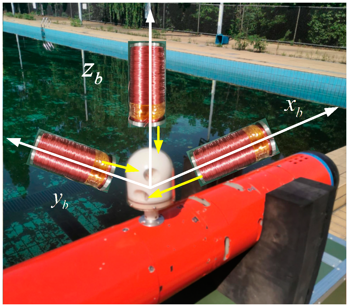
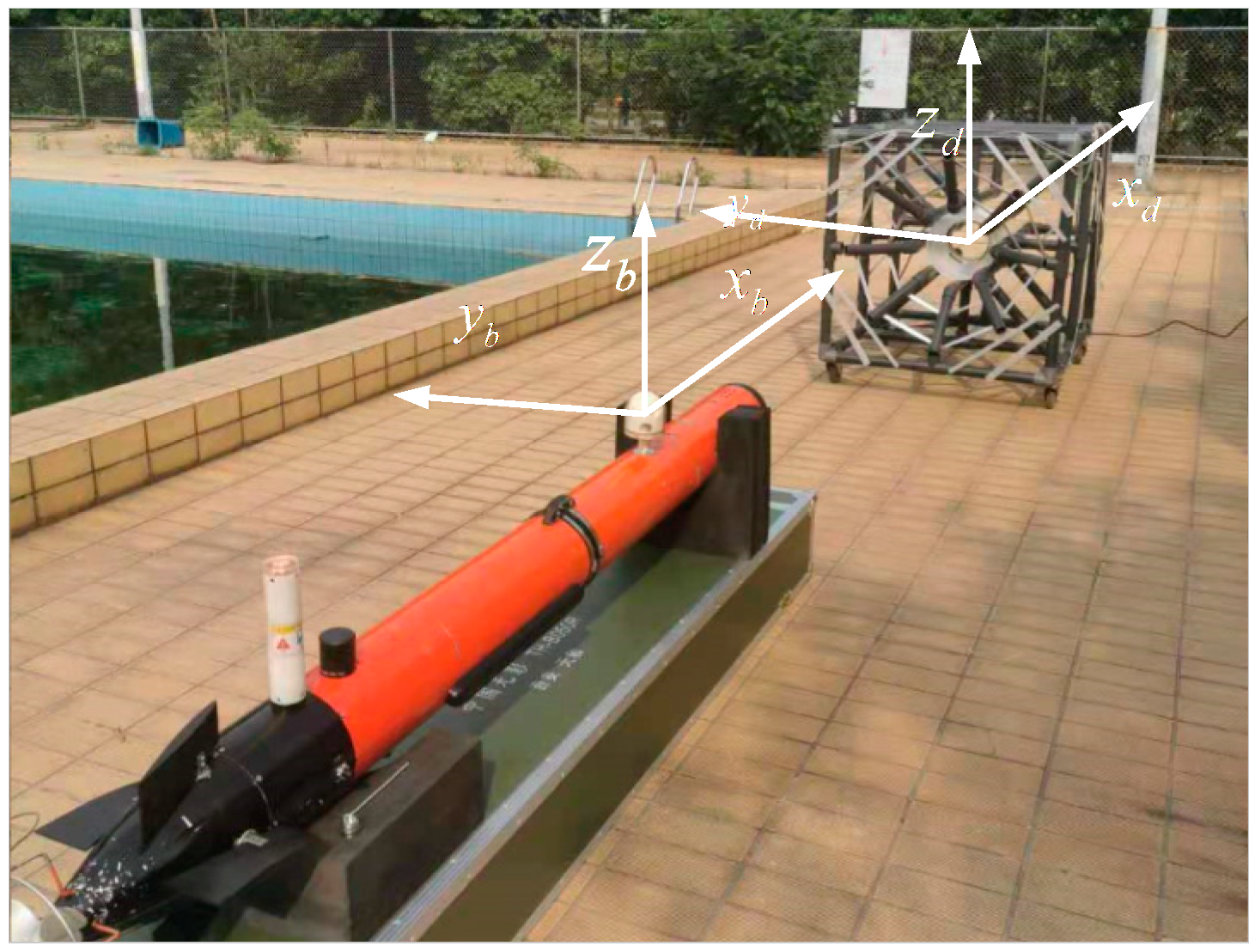
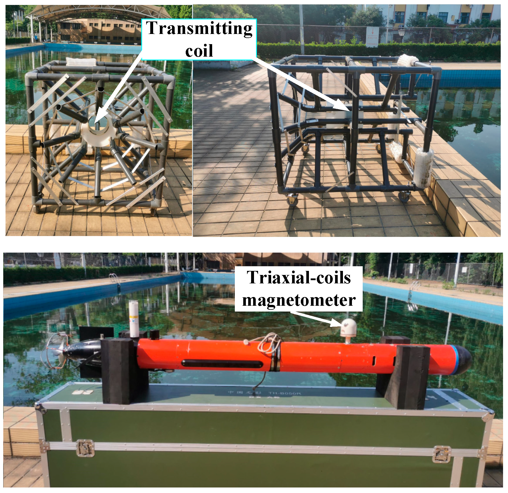
The AUV terminal guidance coordinate system, which includes the fixed coordinates and the body coordinates, is established as shown in Figure 6. The axes of the triaxial-coil magnetometer are allied with the x′-, y′- and z′-axis of the AUV body coordinates. The winding direction of the three coils determined according to the right-hand rule is the same as the direction of their respective coordinate axes. ${\psi }_{yaw},{\psi }_{roll},{\psi }_{pitch}$ are the difference in the yaw angle, roll angle, and pitch angle between the DS and AUV, respectively. The AUV in this paper can maintain a small roll angle and pitch angle during navigation, that is, ${\psi }_{roll}\approx {\psi }_{pitch}\approx 0$. So, the rotation matrix is approximately equal to:

$$R_d^b=R({\psi }_{yaw})R({\psi }_{roll})R({\psi }_{pitch})\approx \left[\begin{array}{ccc}\cos {\psi }_{yaw}& -\sin {\psi }_{yaw}& 0\\ \sin {\psi }_{yaw}& \cos {\psi }_{yaw}& 0\\ 0& 0& 1\end{array}\right],$$

(24)

If a vector ${\mathit{I}}_b={[X_b,Y_b,Z_b]}^T$ is observed in the AUV body coordinate, the vector ${\mathit{I}}_d={[X_d,Y_d,Z_d]}^T$ observed in the fixed coordinate system is:

$${\mathit{I}}_d={(R_d^b)}^T{\mathit{I}}_b,$$

(25)

4.1. Positioning Method Based on Induced Voltage Information of Three-Axis Coils

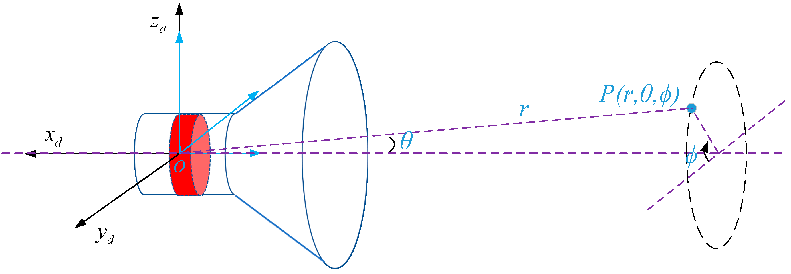
AUV can usually realize fixed depth navigation according to depth control, so the terminal docking guidance can be regarded as the movement in a horizontal plane. Furthermore, in normal terminal guidance, the AUV’s velocity always includes a component towards the positive direction of the x-axis in fixed coordinates. Suppose that the AUV’s depth will be maintained slightly lower than the depth of the DS’s centerline so that the triaxial magnetometer can keep on the horizontal plane of the central axis of the transmitting coil. In this situation, the number of the position solution is reduced to two. The area with the opening angle $2{\theta }_m\approx {109.5}^{\circ }$ in front of the DS is defined as the electromagnetic guidance area. The acoustic guidance in remote homing can guide the AUV into this range, so the setting of this area is reasonable. Since the difference in the yaw angle between AUV and DS during terminal guidance is not equal to 0, the magnetic field vector on the x′- and y′-axis (${\dot{H}}_{x^{\prime }},{\dot{H}}_{y^{\prime }}$) of the magnetometer in body coordinates is not equal to the magnetic field vector on the x- and y-axis (${\dot{H}}_x,{\dot{H}}_y$) of the point in the fixed coordinates. So, the relationship between ${\dot{H}}_x,{\dot{H}}_y$ and ${\dot{H}}_{x^{\prime }},{\dot{H}}_{y^{\prime }}$ is analyzed emphatically here. For the convenience of analysis, the relationship between ${\dot{H}}_x,{\dot{H}}_y$ and ${\dot{H}}_{x^{\prime }},{\dot{H}}_{y^{\prime }}$ is judged by their value at the time $t_0$, at which the current of the transmitting coil reaches a positive amplitude. ${\tilde{H}}_x,{\tilde{H}}_y$ is defined as the value of ${\dot{H}}_x,{\dot{H}}_y$ at time $t_0$, the value of which is $H_x,H_y$ or $-H_x,-H_y$. Similarly, ${\tilde{H}}_{x^{\prime }},{\tilde{H}}_{y^{\prime }}$ is defined as the value of ${\dot{H}}_{x^{\prime }},{\dot{H}}_{y^{\prime }}$ at time $t_0$, the value of which is $H_{x^{\prime }},H_{y^{\prime }}$ or $-H_{x^{\prime }},-H_{y^{\prime }}$.

The position and yaw angle of AUV in the defined terminal electromagnetic guidance area can be divided into eight types, as shown in Figure 7. The relationship between ${\dot{H}}_x,{\dot{H}}_y$ and ${\dot{H}}_{x^{\prime }},{\dot{H}}_{y^{\prime }}$ is shown in

Table 3. The phase between ${\dot{H}}_x$ and ${\dot{H}}_{x^{\prime }}$, the phase between ${\dot{H}}_{x^{\prime }}$ and ${\dot{H}}_{y^{\prime }}$, and the calculation of ${\tilde{H}}_x,{\tilde{H}}_y$ with different yaw angles where $y<0$.

	Situation	Phase between ${\dot{\mathit{H}}}_{\mathit{x}},{\dot{\mathit{H}}}_{{\mathit{x}}^{\mathbf{\prime }}}$	Phase between ${\dot{\mathit{H}}}_{{\mathit{x}}^{\mathbf{\prime }}},{\dot{\mathit{H}}}_{{\mathit{y}}^{\mathbf{\prime }}}$	Calculation of ${\tilde{\mathit{H}}}_{\mathit{x}},{\tilde{\mathit{H}}}_{\mathit{y}}$
(1)	$-\pi /2<{\psi }_{yaw}<-\theta$	In-phase	Anti-phase	$\left[\begin{array}{c}{\tilde{H}}_x\\ {\tilde{H}}_y\end{array}\right]=\left[\begin{array}{cc}\cos {\psi }_{yaw}& -\sin {\psi }_{yaw}\\ \sin {\psi }_{yaw}& \cos {\psi }_{yaw}\end{array}\right]\left[\begin{array}{c}{H}_{x^{\prime }}\\ -H_{y^{\prime }}\end{array}\right]$
(2)	$-\theta <{\psi }_{yaw}<0$	In-phase	In-phase	$\left[\begin{array}{c}{\tilde{H}}_x\\ {\tilde{H}}_y\end{array}\right]=\left[\begin{array}{cc}\cos {\psi }_{yaw}& -\sin {\psi }_{yaw}\\ \sin {\psi }_{yaw}& \cos {\psi }_{yaw}\end{array}\right]\left[\begin{array}{c}{H}_{x^{\prime }}\\ H_{y^{\prime }}\end{array}\right]$
(3)	$0<{\psi }_{yaw}<\pi /2-\theta$	In-phase	In-phase	$\left[\begin{array}{c}{\tilde{H}}_x\\ {\tilde{H}}_y\end{array}\right]=\left[\begin{array}{cc}\cos {\psi }_{yaw}& -\sin {\psi }_{yaw}\\ \sin {\psi }_{yaw}& \cos {\psi }_{yaw}\end{array}\right]\left[\begin{array}{c}{H}_{x^{\prime }}\\ H_{y^{\prime }}\end{array}\right]$
(4)	$\pi /2-\theta <{\psi }_{yaw}<\pi /2$	Anti-phase	In-phase	$\left[\begin{array}{c}{\tilde{H}}_x\\ {\tilde{H}}_y\end{array}\right]=\left[\begin{array}{cc}\cos {\psi }_{yaw}& -\sin {\psi }_{yaw}\\ \sin {\psi }_{yaw}& \cos {\psi }_{yaw}\end{array}\right]\left[\begin{array}{c}-H_{x^{\prime }}\\ H_{y^{\prime }}\end{array}\right]$

and

Table 4. The phase between ${\dot{H}}_x$ and ${\dot{H}}_{x^{\prime }}$, the phase between ${\dot{H}}_{x^{\prime }}$ and ${\dot{H}}_{y^{\prime }}$, and the calculation of ${\tilde{H}}_x,{\tilde{H}}_y$ with different yaw angles where $y>0$.

	Situation	Phase between ${\dot{\mathit{H}}}_{\mathit{x}},{\dot{\mathit{H}}}_{{\mathit{x}}^{\mathbf{\prime }}}$	Phase between ${\dot{\mathit{H}}}_{{\mathit{x}}^{\mathbf{\prime }}},{\dot{\mathit{H}}}_{{\mathit{y}}^{\mathbf{\prime }}}$	Calculation of ${\tilde{\mathit{H}}}_{\mathit{x}},{\tilde{\mathit{H}}}_{\mathit{y}}$
(1)	$\theta <{\psi }_{yaw}<\frac{\pi }{2}$	In-phase	In-phase	$\left[\begin{array}{c}{\tilde{H}}_x\\ {\tilde{H}}_y\end{array}\right]=\left[\begin{array}{cc}\cos {\psi }_{yaw}& -\sin {\psi }_{yaw}\\ \sin {\psi }_{yaw}& \cos {\psi }_{yaw}\end{array}\right]\left[\begin{array}{c}{H}_{x^{\prime }}\\ H_{y^{\prime }}\end{array}\right]$
(2)	$0<{\psi }_{yaw}<\theta$	In-phase	Anti-phase	$\left[\begin{array}{c}{\tilde{H}}_x\\ {\tilde{H}}_y\end{array}\right]=\left[\begin{array}{cc}\cos {\psi }_{yaw}& -\sin {\psi }_{yaw}\\ \sin {\psi }_{yaw}& \cos {\psi }_{yaw}\end{array}\right]\left[\begin{array}{c}{H}_{x^{\prime }}\\ -H_{y^{\prime }}\end{array}\right]$
(3)	$\theta -\frac{\pi }{2}<{\psi }_{yaw}<0$	In-phase	Anti-phase	$\left[\begin{array}{c}{\tilde{H}}_x\\ {\tilde{H}}_y\end{array}\right]=\left[\begin{array}{cc}\cos {\psi }_{yaw}& -\sin {\psi }_{yaw}\\ \sin {\psi }_{yaw}& \cos {\psi }_{yaw}\end{array}\right]\left[\begin{array}{c}{H}_{x^{\prime }}\\ -H_{y^{\prime }}\end{array}\right]$
(4)	$-\frac{\pi }{2}<{\psi }_{yaw}<\theta -\frac{\pi }{2}$	Anti-phase	In-phase	$\left[\begin{array}{c}{\tilde{H}}_x\\ {\tilde{H}}_y\end{array}\right]=\left[\begin{array}{cc}\cos {\psi }_{yaw}& -\sin {\psi }_{yaw}\\ \sin {\psi }_{yaw}& \cos {\psi }_{yaw}\end{array}\right]\left[\begin{array}{c}-H_{x^{\prime }}\\ -H_{y^{\prime }}\end{array}\right]$

where y < 0 and y > 0, respectively.

From the above analysis, it can be seen that only under the conditions that $y<0,\frac{\pi }{2}-\theta <{\psi }_{yaw}<\frac{\pi }{2}$ or $y>0,-\frac{\pi }{2}<{\psi }_{yaw}<\theta -\frac{\pi }{2}$, the phase of ${\dot{H}}_{x^{\prime }}$ is inconsistent with ${\dot{H}}_x$. Therefore, it is necessary to restrict the yaw angle of AUV during the electromagnetic terminal guidance to avoid this situation. Considering that the electromagnetic guidance area is defined as $-{\theta }_m\le \theta \le {\theta }_m,({\theta }_m=a\tan \sqrt{2}\approx {54.7}^{\circ })$, if the restriction $|{\psi }_{yaw}|\le \frac{\pi }{2}-{\theta }_m$ is added to the yaw angle of AUV, then $|{\psi }_{yaw}|\le \frac{\pi }{2}-{\theta }_m\le \frac{\pi }{2}-\theta$ is obtained, that is, ${\dot{H}}_{x^{\prime }}$ remains in-phase with ${\dot{H}}_x$. In the z-axis direction, because the roll angle and pitch angle of the AUV are very small, the magnetic field intensity ${\dot{H}}_{z^{\prime }}$ on the z′ axis of the triaxial-coil magnetometer is basically equal to the magnetic field ${\dot{H}}_z$ in the z-axis in the fixed coordinates. When the triaxial-coil magnetometer moves to the positive direction of the z-axis, ${\dot{H}}_{z^{\prime }}$ is anti-phase with ${\dot{H}}_{x^{\prime }}$ or ${\dot{H}}_x$. On the contrary, when the triaxial-coil magnetometer moves to the negative direction of the z-axis, ${\dot{H}}_{z^{\prime }}$ is in-phase with ${\dot{H}}_{x^{\prime }}$ or ${\dot{H}}_x$. Therefore, the relationship between the magnetic field intensity ${[{\tilde{H}}_{x^{\prime }},{\tilde{H}}_{y^{\prime }},{\tilde{H}}_{z^{\prime }}]}^T$ at time $t_0$ on the triaxial-coil magnetometer and ${[{\tilde{H}}_x,{\tilde{H}}_y,{\tilde{H}}_z]}^T$ in fixed coordinates is:

$$\left[\begin{array}{c}{\tilde{H}}_x\\ {\tilde{H}}_y\\ {\tilde{H}}_z\end{array}\right]=R_b^d\left[\begin{array}{c}{\tilde{H}}_{x^{\prime }}\\ {\tilde{H}}_{y^{\prime }}\\ {\tilde{H}}_{z^{\prime }}\end{array}\right],$$

(26)

According to Formula (22), the amplitude of the magnetic field intensity on each axis can be calculated by the induced voltage amplitude. The phase between the magnetic field of two coil axes can be obtained according to the phase between the induced voltage waveform of the two axes. The matrix $[{\tilde{U}}_x,{\tilde{U}}_y,{\tilde{U}}_z]$ is defined as the amplitude with the polarity of the induced voltage of the triaxial coils detected by the ADC, where ${\tilde{U}}_x=U_x$. If $u_y(t)$ and $u_x(t)$ or $u_z(t)$ and $u_x(t)$ are in-phase, ${\tilde{U}}_y=U_y,{\tilde{U}}_z=U_z$. Meanwhile, if $u_y(t)$ and $u_x(t)$ or $u_z(t)$ and $u_x(t)$ are anti-phase, ${\tilde{U}}_y=-U_y,{\tilde{U}}_z=-U_z$. Therefore, the magnetic field component ${[{\tilde{H}}_{x^{\prime }},{\tilde{H}}_{y^{\prime }},{\tilde{H}}_{z^{\prime }}]}^T$ at time $t_0$ can be expressed as:

$$\left[\begin{array}{c}{\tilde{H}}_{x^{\prime }}\\ {\tilde{H}}_{y^{\prime }}\\ {\tilde{H}}_{z^{\prime }}\end{array}\right]=\left[\begin{array}{c}{\tilde{U}}_x/(A_x{k}_{rx})\\ {\tilde{U}}_y/(A_y{k}_{ry})\\ {\tilde{U}}_z/(A_z{k}_{rz})\end{array}\right],$$

(27)

where $k_{rx}$, $k_{ry}$ and $k_{rz}$ are defined as the receiving parameters of the $x^{\prime }$, $y^{\prime }$, and $z^{\prime }$ axes of the triaxial-coil magnetometer, respectively. The parameter is multiplied by the permeability, the equivalent turns $n$ and the average area $\overline{S}$ of the coil. Taking the receiving parameter $k_{rx}$ on the x′ axis as an example, $k_{rx}=\frac{n\mu \overline{S}}{C_r{R}_r}$. According to Formulas (26) and (27), ${[{\tilde{H}}_x,{\tilde{H}}_y,{\tilde{H}}_z]}^T$ in the fixed-coordinate system is expressed as:

$$\left[\begin{array}{c}{\tilde{H}}_x\\ {\tilde{H}}_y\\ {\tilde{H}}_z\end{array}\right]=R_b^d\left[\begin{array}{c}{\tilde{U}}_x/(A_x{k}_{rx})\\ {\tilde{U}}_y/(A_y{k}_{ry})\\ {\tilde{U}}_z/(A_z{k}_{rz})\end{array}\right],$$

(28)

If ${\dot{H}}_y$ is in-phase ${\dot{H}}_x$, then the polarity of ${\tilde{H}}_y$ is positive; otherwise, the polarity of ${\tilde{H}}_y$ is negative. The phase between ${\dot{H}}_z$ and ${\dot{H}}_x$ is also analyzed in this way. The absolute value of ${[{\tilde{H}}_x,{\tilde{H}}_y,{\tilde{H}}_z]}^T$ and the polarity of ${\tilde{H}}_y,{\tilde{H}}_z$ is utilized to determine the unique position based on the positioning method proposed in Section 2. According to Formula (28), the term $H_z/H_y$ in Formula (12) can be further expressed as:

$$\frac{H_z}{H_y}=\frac{|{\tilde{H}}_z|}{|{\tilde{H}}_y|}=\frac{|\frac{{\tilde{U}}_z}{A_z{k}_{rz}}|}{|\frac{{\tilde{U}}_x}{A_x{k}_{rx}}\sin {\psi }_{yaw}+\frac{{\tilde{U}}_y}{A_y{k}_{ry}}\cos {\psi }_{yaw}|},$$

(29)

The transmitting parameter of the electromagnetic guidance system is defined as $k_t=\frac{M}{2\pi }$, which is only related to the turns, current, and area of the transmitting coil. Therefore, the three axis coils on the magnetometer share the same transmitting parameter. The product of the receiving parameters and transmitting parameter of each coil is defined as a system parameter $k_x,k_y,k_z$. Multiplying the numerator and denominator in Formula (29) by $\frac{1}{k_t}$, Formula (29) is expressed as:

$$\frac{H_z}{H_y}=\frac{|\frac{{\tilde{U}}_z}{A_z{k}_z}|}{|\frac{{\tilde{U}}_x}{A_x{k}_x}\sin {\psi }_{yaw}+\frac{{\tilde{U}}_y}{A_y{k}_y}\cos {\psi }_{yaw}|},$$

(30)

Similarly, the terms $H_x/H_y$ and $M/H_x$ in Formulas (17) and (18) can also transform like $H_z/H_y$ mentioned above, and the final position solution using the induced voltage information is shown below:

$$\varphi ={\varphi }_0,{\varphi }_0+\pi ,\pi -{\varphi }_0,2\pi -{\varphi }_0,\left({\varphi }_0=\mathrm{acrtan}\left(\frac{|\frac{{\tilde{U}}_z}{A_z{k}_z}|}{|\frac{{\tilde{U}}_x}{A_x{k}_x}\sin {\psi }_{yaw}+\frac{{\tilde{U}}_y}{A_y{k}_y}\cos {\psi }_{yaw}|}\right)\right),$$

(31)

$$\theta =\arctan \sqrt{{\left(\frac{3\cos \varphi }{2}\frac{|\frac{{\tilde{U}}_x}{A_x{k}_x}\cos {\psi }_{yaw}-\frac{{\tilde{U}}_y}{A_y{k}_y}\sin {\psi }_{yaw}|}{|\frac{{\tilde{U}}_x}{A_x{k}_x}\sin {\psi }_{yaw}+\frac{{\tilde{U}}_y}{A_y{k}_y}\cos {\psi }_{yaw}|}\right)}^2+2}-\frac{3}{2}\frac{|\frac{{\tilde{U}}_x}{A_x{k}_x}\cos {\psi }_{yaw}-\frac{{\tilde{U}}_y}{A_y{k}_y}\sin {\psi }_{yaw}|}{|\frac{{\tilde{U}}_x}{A_x{k}_x}\sin {\psi }_{yaw}+\frac{{\tilde{U}}_y}{A_y{k}_y}\cos {\psi }_{yaw}|}|\cos \varphi |,$$

(32)

$$r=\sqrt[3]{\frac{(2{\cos }^2\theta -{\sin }^2\theta )}{2|\frac{{\tilde{U}}_x}{A_x{k}_x}\cos {\psi }_{yaw}-\frac{{\tilde{U}}_y}{A_y{k}_y}\sin {\psi }_{yaw}|}},$$

(33)

.

According to Formula (33), if each coil in the magnetometer is placed on the axis of the transmitting coil with its axis coinciding with the axis of the transmitting coil, the system parameter of each coil in the receiver can be obtained by the amplitude $U_{r_m}$ of the induced voltage and distance $r_m$:

$$k_i=\frac{U_{r_m}{r}_m^3}{A_i},i=x,y,z$$

(34)

4.2. Guidance Control Strategy

The terminal guidance diagram of an AUV in the northeast sky coordinate is shown in Figure 8. The yaw angle of the DS and the AUV is defined as ${\psi }_{Dock}$ and ${\psi }_{AUV}$, respectively. Then, the yaw difference ${\psi }_{yaw}$ between AUV and DS is:

$${\psi }_{yaw}={\psi }_{AUV}-{\psi }_{Dock},$$

(35)

We define the angle $\phi$ as the direction angle between the center line of the DS and the line connecting the triaxial-coil magnetometer and the origin point of the fixed coordinate system. The measured direction angle is related to the coordinates (x, y) calculated by the triaxial-coil magnetometer:

$$\phi =\arctan \frac{y}{x},$$

(36)

As shown in Figure 8, the angle difference $\Delta \phi$ between the AUV’s yaw angle and the line connecting the triaxial-coil magnetometer is defined, and the origin point of the fixed-coordinate system is:

$$\Delta \phi ={\psi }_{yaw}-\phi ,$$

(37)

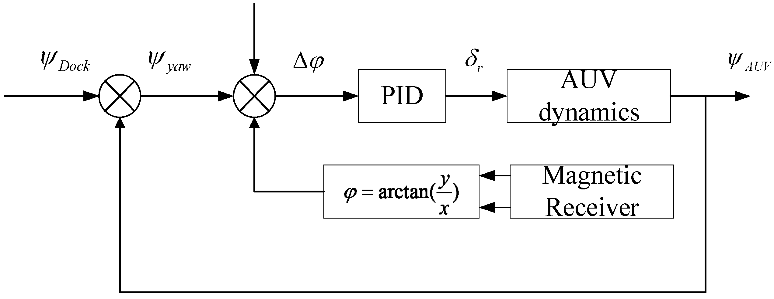
The angle $\Delta \phi$ being equal to 0 means that the AUV tracks the line connecting the triaxial-coil magnetometer and the origin point of the fixed coordinate, and it will finally enter the DS. The docking control strategy to adjust the angle $\Delta \phi$ to 0 by adjusting the horizontal rudder of the AUV is shown in Figure 9. Since the DS is fixed underwater, the yaw angle of the DS will not change. The AUV obtains the current yaw deviation by the compass, then calculates the current coordinates and direction angle in the fixed-coordinate system based on the data from the triaxial-coil magnetometer. The difference $\Delta e$ between the angle $\Delta \phi$ and 0 is the control quantity of the system. It is changed into the required steering angle ${\delta }_r$ by using the PID controller, and then the AUV is controlled to continuously track the origin of the DS in terminal docking guidance.

5. Configuration of the Electromagnetic Guidance System

The electromagnetic guidance system in this paper is divided into two parts: the electromagnetic transmitter and receiver. The function of the electromagnetic transmitter is to generate an electromagnetic field of sufficient strength. The electromagnetic receiver performs a positioning calculation by the detected magnetic field strength, so as to provide AUV terminal docking guidance. The prototype of the electromagnetic guidance system is shown in Figure 10.

5.1. Electromagnetic Transmitter

The electromagnetic transmitter includes the transmitting coil and its driving circuit. The radius of the coil is 100 mm, which is much smaller than the distance between the AUV and itself in terminal docking guidance, so the magnetic dipole model is applicable. A Litz wire with a line diameter of 1.5 mm is used to wind the transmitting coil. The parameters of the transmitting coil are shown in

Table 5. Parameters of transmitting coil.

Parameter	Value
Turns	42
Self-inductance	460 uH
Line diameter	1.5 mm
Diameter	200 mm
Resistor	0.8 ohms

.

The driving circuit in this paper includes a signal generator, power amplifier, LCC resonant circuit, and transmitting coil, as shown in Figure 11. The signal generator can generate a weak AC signal to drive the transmitting coil. Therefore, the power amplifier connected with the signal generator is used to enlarge the voltage of the AC so that it can generate a larger coil current. If it is directly connected to the transmitting coil, the output current of the power amplifier will be very small due to the great self-inductance of the coil itself. The LCC resonant circuit is added to match the impedance of the whole system and further amplify the current [20,21]. By controlling the output voltage of the signal generator, a linear change in the coil current within 0 A~4.16 A can be realized.

5.2. Electromagnetic Receiver

The electromagnetic receiver contains the triaxial-coil magnetometer, signal-processing circuit, compass, and main controller of the AUV, as shown in Figure 12. The design of the triaxial-coil magnetometer is introduced in Section 4. The triaxial coils are installed in a plastic fastener with magnetic permeability. After watertight treatment, the magnetometer is connected to the cabin of the AUV. The induced voltage of the triaxial-coil magnetometer can be transformed into a signal collected by the ADC only after passing through the signal-processing circuit. The schematic diagram of the signal-processing circuit is shown in Figure 12. The programmable gain amplification (PGA) chip AD8231 is used to amplify the induced voltage of the three coils in this paper. This module is able to amplify a bipolar voltage with a voltage gain ranging from 1 to 2⁷. Furthermore, the output voltage range of the PGA is $-2.5\mathrm{V}~2.5\mathrm{V}$. Two PGA modules are adopted in each channel to expand the range of voltage gain. The signal is filtered by the band-pass filter for which cut-off frequencies of the band-pass filter are 500 Hz and 5 kHz after each amplification. Finally, the bipolar signal enters the 16-bit ADC (AD7606) for three-channel data acquisition and caching. The sampling frequency of the three channels is set to 51,200 Hz, and 256 data points are collected at the same time in each channel. When the number of data points of each axis reaches 256, the collected data are transmitted to STM32f407 through a serial port. Then, STM32f407 extracts the FFT results and phase information of the data. The gain in the PGA modules of each channel is adjusted according to the max amplitude from the FFT results. The amplitude of the induced voltage of the three coils and the phase information are sent to the main controller of the AUV for positioning and motion control.

6. Experiment

6.1. Positioning Test

The current amplitude of the transmitting coil is set as 2.5 A and the frequency is 1 kHz. The electromagnetic module is tested underwater, as shown in Figure 13. Before positioning with the electromagnetic guidance system, it is necessary to obtain the three axis system parameters $k_x,k_y,k_z$. The method of obtaining the system parameters is shown in Formula (34). The results are shown in

Table 6. System parameters calculated for each axis at different distances.

	1 m	2 m	3 m	4 m	5 m	6 m	7 m	Mean
x-coil	0.1732	0.1798	0.1848	0.1907	0.1884	0.1869	0.1771	0.1830
y-coil	0.1747	0.1847	0.1950	0.1951	0.1982	0.2012	0.2003	0.1927
z-coil	0.1904	0.1873	0.1976	0.1995	0.1978	0.2008	0.2004	0.1963

.

Considering that, during AUV terminal docking, the depth meter is used to determine the depth in the vertical direction and the AUV is equivalent to docking on a plane, the positioning test is also carried out on a horizontal plane, and the triaxial-coil magnetometer is placed on the plane where the central axis of the transmitting coil is located. The positioning test of the electromagnetic guidance system is divided into the static positioning test and the dynamic positioning test. In the static positioning test, the triaxial coils are parallel to the three axes of the fixed coordinate system. The triaxial-coil magnetometer is placed within the area of 10 m × 4 m in front of the transmitting coil for the positioning test. A total of 500 groups of positioning data are recorded at different points with a sampling frequency of 35 Hz. Every seven points of positioning data are filtered by removing the maximum and minimum values, so the actual positioning frequency is 5 Hz.

The results of static positioning are shown in Figure 14, which shows that the effective range of electromagnetic positioning can reach 10 m. With the increase in distance r and angle θ, the error between the calculated position and the real test points and the fluctuation range of the calculated position also gradually increase. According to the filtered positioning data, the noise level at each point for which the x-coordinate is equal to −6 m is shown in Figure 15. It is seen that the calculated RMSE of distance r and coordinate (x, y) is less than 10 cm. If the x-coordinate is bigger than −6 m, the positioning RMSE is smaller, which means the positioning is more accurate. In order to ensure the positioning accuracy of AUV terminal docking, the electromagnetic guidance area is determined as the area where −6 ≤ x < 0. Within this range, the electromagnetic positioning accuracy can reach the centimeter level.

The module moves with a speed of 0.5 m/s along a rectangular trajectory that contains points (−2, −2), (−5, −2), (−5, 2), and (−2, 2). The module starts from point (−2, −2), passes through points (−5, −2), (−5, 2), and (−2, 2), and finally stops at point (−2, −2). During the whole process, the orientation angle of the receiver is constantly changed between −30 and 30 degrees, as detected by a compass. The trajectory calculated by the electromagnetic guidance module is basically consistent with the real rectangular trajectory, as shown in Figure 16. The error between the calculated position and the real position is shown in Figure 17. It can be seen that the positioning error tends to increase gradually when the electromagnetic guidance module is far away from the transmitting coil. During the whole movement, the maximum positioning error of the x-coordinate and y-coordinate is approximately 0.2 m. Additionally, the positioning error of angle θ and distance r is less than 2.5 deg and 0.2 m, respectively.

6.2. AUV Terminal Docking Experiment

The transmitter and receiver of the electromagnetic guidance module developed in this paper are installed on the DS and AUV, respectively, as shown in Figure 18. The DS is made of PVC material and the AUV is of the torpedo type, with a diameter of 180 cm and a steady speed of 1 m/s. The DS is employed in the swimming pool, and the centerline of the transmitting coil is at a depth of 0.5 m. Therefore, the navigating depth of the AUV is 0.65 m so that the magnetometer can keep on the horizontal plane where the centerline of the transmitting coil is located during AUV docking. The area of electromagnetic guidance is the area with an opening angle of $2{\theta }_m$ in front of the DS and an x-coordinate greater than −6 m. Five underwater terminal docking tasks are carried out, and four of them are successfully completed. The reason for the failure is that the initial yaw angle of the AUV is too large, such that the AUV cannot enter the terminal electromagnetic guidance area. One of the successful trajectories is shown in Figure 19, and the docking process is shown in Figure 20. As the AUV navigates underwater in the swimming pool, GPS and USBL cannot be used for positioning. Therefore, the AUV’s navigation trajectory is mainly calculated according to the velocity and yaw angle of the AUV. The change in the trajectory (Figure 21a) obtained from the electromagnetic field information is basically consistent with the AUV’s track calculated by the velocity and yaw angle (Figure 19). When the triaxial-coil magnetometer on the AUV detects that the calculated x-coordinate is greater than -6 m, the electromagnetic guidance begins to work. An obvious change can be seen from the yaw angle of the AUV in Figure 21b, which indicates that electromagnetic guidance causes the effect.

7. Discussion

Compared with optical/visual guidance, electromagnetic guidance can be applied to instances with strong background light and muddy water quality. Furthermore, in order to increase the range of optical/guidance, the energy consumption of the underwater lamp applied is usually large, so as to increase the brightness of the underwater lamp. In the literature [3,13], the power of a light reaches more than 100 W. The power of the transmitter of the electromagnetic guidance in this paper is approximately 30 W, which is greatly reduced compared with the power of the underwater lamp. Other institutions have also conducted research related to AUV electromagnetic guidance technology. A comparison between the electromagnetic guidance developed in this paper and by other institutions is shown in

Table 7. Comparison of electromagnetic guidance schemes (five solid stars indicate full marks).

	Feezor et al. [8]	Vandavasi et al. [14]	Shilin P et al. [15,16]	Daegel Park et al. [17,18]	This Paper
Volume	With large transmitter	Small size	With large transmitter	Small size	Small size
	(★★★★☆)	(★★★★★)	(★★★★☆)	(★★★★★)	(★★★★★)
Effective range	25–30 m	7 m	20 m	6 m	10 m
	(★★★★★)	(★★★☆☆)	(★★★★★)	(★★★☆☆)	(★★★★☆)
Low cost?	Yes	No (two magnetometers with relatively high price)	Yes	No (transmitter and receiver with relatively high price)	Yes
	(★★★★★)	(★★★★☆)	(★★★★★)	(★★★☆☆)	(★★★★★)
Easy to install?	No (transmitting coil with large size)	Yes	No (transmitting coil with large size)	No (4 transmitters should be installed near the DS with high installation accuracy)	Yes
	(★★★★☆)	(★★★★★)	(★★★★☆)	(★★★★☆)	(★★★★★)
Positioning function	N/A	N/A	N/A	Positioning with high accuracy (specific precision value not mentioned)	Positioning accuracy reaches centimeter level within the range of 6 m
				(★★★★★)	(★★★★★)
Experimental conditions	Sea test	Pool test on water surface with a micro AUV prototype	Pool test on water surface with a micro AUV prototype	Underwater pool test with an ROV	Underwater swimming pool test with AUV docking system
	(★★★★★)	(★★★★☆)	(★★★★☆)	(★★★★★)	(★★★★★)
AUV docking success rate	5/8 (62.5%)	N/A	N/A	N/A	4/5 (80%)
	(★★★★☆)				(★★★★☆)

. Each scheme has its own advantages and disadvantages. However, considering the volume, effective range, cost, experimental condition, installation difficulty, positioning function, and AUV docking success rate of the electromagnetic guidance scheme, the comprehensive score of the scheme proposed in this paper is relatively high.

In the future, our research work will focus on the following:

• The guidance range of the electromagnetic guidance with centimeter-level accuracy presented in this paper is relatively short. In order to improve this range, it is necessary to further strengthen the anti-interference performance of the signal-processing circuit to increase the positioning accuracy. In this way, a longer guidance range can meet the accuracy requirement.
• The accuracy of electromagnetic positioning in this paper can be further improved by some positioning filtering algorithms, such as the extended Kalman filter and particle filter.
• The application value of the terminal electromagnetic guidance method can be further verified in sea trials.

8. Conclusions

An underwater terminal electromagnetic guidance method based on the magnetic dipole model is proposed in this paper. A transmitting coil with an AC current of 1 kHz is utilized to generate an electromagnetic field. Based on the magnetic dipole model, the electromagnetic field in the terminal guidance range is the near field where the position can be obtained through the amplitude and phase relationships of three orthogonal magnetic field vectors. A magnetometer with three orthogonal coils and a method for extracting the amplitude and phase of the induced voltage are proposed in this paper. According to Faraday’s law, the relationship between the induced voltage and the magnetic field intensity is obtained, so the amplitude and phase information of the induced voltage of the three coils on the triaxial-coil magnetometer is used to determine the position. The underwater positioning test shows that the effective range of the electromagnetic guidance system can reach 10 m. The RMSE of the positioning in the area of 4 m × 6 m in front of the transmitting coil can be lower than 1 cm. Five underwater terminal docking tasks were carried out, and four of them were successfully completed, which verified the electromagnetic guidance proposed in this paper. The highlights of this article can be summarized as follows:

(1)

Based on the magnetic dipole model, the distribution of a low-frequency electromagnetic field excited by the coil is obtained. Then, the positioning method is analyzed according to the amplitude and relative phase of the magnetic field intensity.

(2)

A triaxial-coil magnetometer and the method for extracting the amplitude and phase of the induced voltage are presented in this paper. Furthermore, a method based on the induced voltage information of a triaxial-coil magnetometer is proposed to replace the information on magnetic field intensity in relation to positioning.

References

1. Hurtós, N.; Mallios, A.; Palomeras, N.; Bosch, J.; Vallicrosa, G.; Vidal, E.; Ribas, D.; Gracias, N.; Carreras, M.; Ridao, P. LOON-DOCK: AUV homing and docking for high-bandwidth data transmission. In Proceedings of the OCEANS 2017—ABERDEEN. 2017: Oceans Aberdeen Conference, Aberdeen, UK, 19–22 June 2017. [Google Scholar]
2. Li, D.J.; Chen, Y.H.; Shi, J.G.; Yang, C.J. Autonomous underwater vehicle docking system for cabled ocean observatory network. Ocean. Eng. 2015, 109, 127–134. [Google Scholar] [CrossRef]
3. Lin, R.; Li, D.; Zhang, T.; Lin, M. A non-contact docking system for charging and recovering autonomous underwater vehicle. J. Mar. Sci. Technol. 2019, 24, 902–916. [Google Scholar] [CrossRef]
4. Stokey, R.; Purcell, M.; Forrester, N.; Austin, T.; Goldsborough, R.; Allen, B.; von Alt, C. A docking system for REMUS, an autonomous underwater vehicle. In Proceedings of the Oceans ’97, MTS/IEEE Conference Proceedings, Halifax, NS, Canada, 6–9 October 2002. [Google Scholar]
5. Allotta, B.; Caiti, A.; Costanzi, R.; Fanelli, F.; Fenucci, D.; Meli, E.; Ridolfi, A. A new AUV navigation system exploiting unscented Kalman filter. Ocean. Eng. 2016, 113, 121–132. [Google Scholar] [CrossRef]
6. Paull, L.; Saeedi, S.; Seto, M.; Li, H. AUV Navigation and Localization: A Review. IEEE J. Ocean. Eng. 2014, 39, 131–149. [Google Scholar] [CrossRef]
7. Lin, R.; Zhang, F.; Li, D.; Lin, M.; Zhou, G.; Yang, C. An Improved Localization Method for the Transition between Autonomous Underwater Vehicle Homing and Docking. Sensors 2021, 21, 2468. [Google Scholar] [CrossRef] [PubMed]
8. Feezor, M.D.; Sorrell, F.Y.; Blankinship, P.R.; Bellingham, J.G. Autonomous underwater vehicle homing/docking via electromagnetic guidance. Ocean. Eng. IEEE J. Ocean. Eng. 2001, 26, 515–521. [Google Scholar] [CrossRef]
9. McEwen, R.S.; Hobson, B.W.; McBride, L.; Bellingham, J.G. Docking Control System for a 54-cm-Diameter (21-in) AUV. IEEE J. Ocean. Eng. 2008, 33, 550–562. [Google Scholar] [CrossRef]
10. Tan, H.P.; Diamant, R.; Seah, W.K.; Waldmeyer, M. A survey of techniques and challenges in underwater localization. Ocean. Eng. 2011, 38, 1663–1676. [Google Scholar] [CrossRef] [Green Version]
11. Vaganay, J.; Baccou, P.; Jouvencel, B. Homing by acoustic ranging to a single beacon. In Proceedings of the OCEANS 2000 MTS/IEEE Conference and Exhibition. Conference Proceedings (Cat. No.00CH37158), Providence, RI, USA, 11–14 September 2000. [Google Scholar]
12. Sutantyo, D.; Buntoro, D.; Levi, P.; Mintchev, S.; Stefanini, C. Optical-guided autonomous docking method for underwater reconfigurable robot. In Proceedings of the IEEE International Conference on Technologies for Practical Robot Applications, Woburn, MA, USA, 22–23 April 2013. [Google Scholar]
13. Li, D.; Zhang, T.; Yang, C. Terminal Underwater Docking of an Autonomous Underwater Vehicle Using One Camera and One Light. Mar. Technol. Soc. J. 2016, 50, 58–68. [Google Scholar] [CrossRef]
14. Vandavasi, B.N.J.; Arunachalam, U.; Narayanaswamy, V.; Raju, R.; Vittal, D.P.; Muthiah, R.; Gidugu, A.R. Concept and testing of an electromagnetic homing guidance system for autonomous underwater vehicles. Appl. Ocean Res. 2018, 73, 149–159. [Google Scholar] [CrossRef]
15. Peng, S.; Liu, J.; Wu, J.; Li, C.; Liu, B.; Cai, W.; Yu, H. A Low-Cost Electromagnetic Docking Guidance System for Micro Autonomous Underwater Vehicles. Sensors 2019, 19, 682. [Google Scholar] [CrossRef] [PubMed] [Green Version]
16. Wu, J.; Peng, S.; Xu, T.; Hu, R.; Wang, S.; Pan, M.; Weng, X. Test Bed AUV for Docking Algorithm Research. In Proceedings of the OCEANS 2018 MTS/IEEE Charleston, Charleston, SC, USA, 22–25 October 2018. [Google Scholar]
17. Park, D.; Jung, J.; Kwak, K.; Chung, W.K.; Kim, J. 3D underwater localization using EM waves attenuation for UUV docking. In Proceedings of the 2017 IEEE Underwater Technology (UT), Busan, Korea, 21–24 February 2017. [Google Scholar]
18. Park, D.; Kwak, K.; Chung, W.K.; Kim, J. Development of Underwater Short-Range Sensor Using Electromagnetic Wave Attenuation. IEEE J. Ocean. Eng. 2016, 41, 318–325. [Google Scholar]
19. Roux, A.; Le Contel, O.; Coillot, C.; Bouabdellah, A.; De La Porte, B.; Alison, D.; Ruocco, S.; Vassal, M.C. The Search Coil Magnetometer for THEMIS. Space Sci. Rev. 2008, 141, 265–275. [Google Scholar] [CrossRef] [Green Version]
20. Li, S.; Li, W.; Deng, J.; Nguyen, T.D.; Mi, C.C. A Double-Sided LCC Compensation Network and Its Tuning Method for Wireless Power Transfer. IEEE Trans. Veh. Technol. 2015, 64, 2261–2273. [Google Scholar] [CrossRef]
21. Kan, T.; Nguyen, T.D.; White, J.C.; Malhan, R.K.; Mi, C.C. A New Integration Method for an Electric Vehicle Wireless Charging System Using LCC Compensation Topology: Analysis and Design. IEEE Trans. Power Electron. 2017, 32, 1638–1650. [Google Scholar] [CrossRef]
Figure 1. The spherical coordinate and fixed rectangular coordinate defined in the DS. The red part indicates the transmitting coil, which is installed on the DS. The origin of the spherical coordinate system and fixed coordinate system are established on the center point of the coil. The direction of the x-axis and z-axis in the fixed coordinates points to the back and vertically above the DS, respectively.
Jmse 10 00995 g001
Figure 2. The distribution of four solutions of angle ϕ in the y o z plane.
Jmse 10 00995 g002
Figure 3. The distribution of the magnetic field vector of a point in front of the transmitting coil where the x-coordinate is negative; (a) is the plane x o y , and (b) is the plane x o z .
Jmse 10 00995 g003
Figure 4. The composition and installation of the triaxial-coil magnetometer in AUV body coordinates.
Jmse 10 00995 g004
Figure 5. Equivalent circuit of the coil and signal-processing circuit.
Jmse 10 00995 g005
Figure 6. The fixed coordinates ( o x d y d z d ) and body coordinates ( o x b y b z b ) defined in AUV terminal docking.
Jmse 10 00995 g006
Figure 7. Distribution of magnetic field vectors at the point where the triaxial-coil magnetometer is located at time t 0 with different yaw angles (upper: where y < 0; lower: where y > 0).
Jmse 10 00995 g007
Figure 8. The terminal guidance diagram of an AUV in the northeast sky coordinates.
Jmse 10 00995 g008
Figure 9. AUV motion control diagram.
Jmse 10 00995 g009
Figure 10. The prototype of the electromagnetic guidance system. Left and right are the electromagnetic transmitter and receiver, respectively.
Jmse 10 00995 g010
Figure 11. Schematic diagram of the coil drive circuit.
Jmse 10 00995 g011
Figure 12. Configuration of the electromagnetic receiver.
Jmse 10 00995 g012
Figure 13. Underwater scene of electromagnetic positioning module.
Jmse 10 00995 g013
Figure 14. Underwater static positioning results (the green points are the original positioning data; the red points are the filtered positioning data; the blue points are the test points).
Jmse 10 00995 g014
Figure 15. The positioning noise level of electromagnetic positioning, where the x-coordinate is equal to −6 m.
Jmse 10 00995 g015
Figure 16. Dynamic positioning test of rectangular trajectory.
Jmse 10 00995 g016
Figure 17. Positioning error in dynamic positioning test; (a) is the positioning error of θ and r, and (b) is the positioning error of the x and y coordinates.
Jmse 10 00995 g017
Figure 18. The DS and AUV with an electromagnetic guidance module in the docking experiment.
Jmse 10 00995 g018
Figure 19. AUV trajectory of successful docking (green: calculated by the velocity and yaw angle; red: electromagnetic positioning).
Jmse 10 00995 g019
Figure 20. Picture sequence of the AUV docking process.
Jmse 10 00995 g020
Figure 21. The trajectory of the electromagnetic positioning (x, y) (a) and AUV’s yaw angle (b) during AUV terminal docking.
Jmse 10 00995 g021