Numerical Study of Wave Drift Load and Turning Characteristics of KVLCC2 Ship in Regular Waves Based on TEBEM

Abstract

Maritime traffic has increased considerably in recent years, making energy efficiency and navigation safety of ships more crucial than ever. Hence, a two-time scale model based on the Taylor expansion boundary element method (TEBEM) is proposed to predict ship turning trajectories in regular waves. The maneuvering motion is calculated using a three degrees of freedom MMG model that considers the wave drift loads. TEBEM overcomes the shortcomings of the constant panel method in solving tangential induced velocity at a non-smooth boundary and that of the high-order boundary element method in dealing with a high-order derivative of the velocity potential at the corner. This significantly improves the calculation accuracy of the induced velocity and high-order derivative of velocity potential. Firstly, based on the TEBEM, the surge and sway wave drift forces and yaw moment of the KVLCC2 model with drift angle under full wave headings are calculated and compared with computational fluid dynamics results, using which the calculation accuracy of TEBEM is verified. Subsequently, the two-time scale model is used to calculate the turning trajectories of the KVLCC2 model in regular waves with different wave headings, wave frequencies, and wave steepness. The numerical results show that the drift angle has a certain effect on the wave drift loads of the ship, and the proposed model can effectively predict the ship’s turning motion in regular waves.

1. Introduction

With the recent increase in maritime traffic, energy efficiency, and navigation safety of ships have become crucial, and ship coupled hydrodynamic performance analysis has become a research focus. In the early stages of the development of ship hydrodynamics, limited by theoretical models and computational power, some assumptions and simplifications must be made to conduct studies on ship hydrodynamics. Presently, the study of ship seakeeping mainly focuses on the wave drift loads at zero drift angle. However, the ship usually has a certain drift angle when moving under actual sea conditions, affecting the calculation of wave drift loads. Ship maneuverability prediction is typically conducted under calm water conditions, but during actual sea navigation, the seakeeping and the maneuvering motions occur simultaneously and affect each other. The International Towing Tank Conference (ITTC) set up a special committee on ship maneuvering in waves to review the advances in analyzing the coupled motion of ship maneuvering and seakeeping. At present, the popular coupling analysis methods for ship maneuvering and seakeeping can be divided into the following: experimental method, numerical simulation using computational fluid dynamics (CFD), numerical simulation based on the unified theory, and numerical simulation based on two-time-scale models.

The physical tank model test is the most reliable method to study the hydrodynamic performance of ships. The most representative experimental research is the work of Yasukawa’s group at Hiroshima University [1,2,3,4], which investigated ship maneuverability in waves in a physical tank on SR108 and S175 container ship models and a KVLCC2 ship model. Xu et al. [5] and Kinoshita et al. [6] conducted planar motion mechanism (PMM) tests in waves to measure the hydrodynamic force and horizontal displacement of the ship, thereby analyzing the influence of the low-frequency wave drift forces on the ship maneuvering. Lee et al. [7] used a KVLCC model to determine the trajectory for the turning and zigzag maneuvers in regular waves with different wave heights and wavelengths. The test results show that second-order wave forces significantly impact ship maneuverability. Kim et al. [8] also conducted a tank-based study on ship maneuvering of a KVLCC2 ship in regular waves and analyzed the influence of wave heading, wave frequency, and wave steepness on the turning motion. These experiments also provide comparative analysis and validation criteria for numerical models of ship maneuvering prediction in waves.

With the recent increase in computational power, the CFD method has been adopted by the industry for the modeling of ship hydrodynamic performance. High accuracy can be achieved, with results being within 3% of the test results from a physical tank, especially in calm water. However, using the CFD method to simulate ship maneuvering directly in waves remains time-consuming. Kim et al. [9] used the Reynolds-averaged Navier–Stokes (RANS) solver to numerically simulate PMM maneuvering motion to obtain hydrodynamic derivatives of ship maneuvering. Shang et al. [10] used the overlapping grid technology and a propeller volumetric force model to realize numerical prediction of zigzag maneuvers in calm water conditions. Ma et al. [11] conducted numerical and physical tank studies on ship PMM movement in regular waves using the URANS (Unsteady RANS) viscous flow solution and overlapping grid technology.

Numerical simulation based on the two-time scale model and unified theory is more widely used than the CFD method. Both methods are based on the potential flow theory but differ in their treatment of the details. The method based on the unified theory adopts the 6 degrees of freedom (6-DOF) motion equation of the ship in calm water; the F-K, radiation, and diffraction forces caused by the waves are included in the equation as external forces, resulting in a set of unified 6-DOF rigid body motion equations to describe the ship’s motion in the waves. Hamamoto and Kim [12] proposed the horizontal body-fixed coordinate system, thus simplifying the 6-DOF motion description of ships in waves. Sutulo and Soares [13] proposed an auxiliary state variable method to simplify the calculation of the convolution integral in the “memory effect.” Fang et al. [14] calculated the additional mass and damping of the ship according to the instantaneous encounter frequency in the ship’s turning process and proposed a nonlinear model to calculate the ship’s turning trajectory in waves. Lin et al. [15] expanded LAMP, a three-dimensional seakeeping software, and conducted numerical prediction of the maneuverability of various ship models in waves. Subramanian and Beck [16] proposed a body-exact strip theory to simulate the maneuvering of a ship in a seaway, in which the wave drift load effects were considered via the square of the velocity potential gradient. Based on the model proposed by Hamamoto and Kim [12], Suzukie et al. [17] formed their own model by improving the external wave forces and the inertial and damping components of the hydrodynamic forces induced and simulated the turning motion of the KVLCC1 and KCS models in regular waves.

Although numerical simulation methods based on unified theory can consider the effect of wave drift forces, the calculation usually requires some approximation. Therefore, their calculation accuracy is often difficult to guarantee. In comparison, the two-time scale method has some advantages in calculating the wave drift forces. The two-time scale method divides the total ship motion into ship maneuvering and wave-induced motions, which are described by two different sets of motion equations. Seo and Kim [18], Zhang and Zou [19], and Xie et al. [20] built a prediction model of the ship’s turning and maneuvering motion in waves based on the two-time scale method and three-dimensional potential flow theory. Yao et al. [21] used the two-time scale method to construct a prediction model of ship maneuvering in waves, but the difference is that a time-average model is proposed for the prediction model of ship seakeeping. Mei et al. [22] also built a coupled prediction model of ship motion using the two-time scale model. They used the RANS viscous flow CFD method to calculate the hydrodynamic derivative of the ship and the three-dimensional potential flow theory to predict wave drift loads. Jeon M. et al. [23] used EBM method to construct a fast prediction model of ship wave drift load, which was coupled with the 3-DOF MMG motion equation to form a ship handling motion prediction model in waves. Yasukawa et al. [24] calculated the wave-induced steady forces by using the zero-speed three-dimensional panel method and the wave-induced force formula based on the Cochin function of a hypothetical slender ship. Zhang et al. [25] calculated the 6-DOF motions and second-order wave drift force and moment of the KVLCC2 Tanker and S-175 Container ship in waves by using the near-field integral formula.

Presently, the seakeeping of ships is mainly calculated by the constant surface element method and the high-order boundary element method (HOBEM) based on the three-dimensional potential flow theory. The constant surface element method is widely used because of its straightforward programming. However, it yields low accuracy in solving velocity potential and tangential induced velocity at the non-smooth boundary. Compared with the constant boundary element method, HOBEM improves the calculation accuracy under the same number of panel elements. Nevertheless, the calculation accuracy is often lower when the boundary has sharp angles and the higher-order derivative of the velocity potential is needed. Thus, in this study, the Taylor expansion boundary element method (TEBEM) is proposed to solve the velocity field and higher-order derivative field of the boundary value problem of the arbitrary flow field, thereby significantly improving the numerical accuracy of wave drift loads. Moreover, the two-time scale model based on TEBEM exhibits excellent numerical accuracy and computational efficiency in calculating the turning motion of ships in waves.

In this study, based on the Taylor expansion boundary element method (TEBEM) (Duan et al.) [26], the 6-DOF motions and wave drift loads of the KVLCC2 model with drift angle are calculated in oblique waves and compared with the CFD calculation results. The comparison results show that the two methods are in good agreement, thus verifying the accuracy of TEBEM for calculating wave drift loads. Then, based on the two-time scale model, the turning trajectory of a KVLCC2 ship is calculated in regular waves with different wave headings, wave frequencies, and wave steepness. The numerical simulation results agree with the experimental results reported by Kim et al. [8].

2. Two-Time Scale Model

In this study, the hydrodynamic problems of ships are addressed via potential flow theory. The total ship motion is divided into low-frequency ship maneuvering and high-frequency wave-induced motions, and the two are coupled with each other. The low-frequency motion is affected by the second-order wave drift loads, which indirectly depend on the ship’s wave-induced motion. Conversely, the high-frequency motion changes with the ship’s speed and heading angle, which must be determined by solving the low-frequency motion. Therefore, this study constructs a mathematical model of the ship’s maneuvering motion based on the two-time scale model. In the numerical calculation, the following steps are adopted to deal with the coupling solution of the two sets of equations:

(1)

The time domain TEBEM is used to solve the boundary value problem of the ship at its initial velocity and position. Subsequently, the first-order hydrodynamic force is obtained by the pressure integration on the wet surface of the ship, and the high-frequency motion of the ship is obtained using the wave-induced 6-DOF motion equations. Finally, the wave drift forces and moment are directly calculated using the near-field integral method;

(2)

The boundary value problem of the ship is updated via the high-frequency motion obtained in step (1). Subsequently, the time domain TEBEM is used to solve the new boundary value problem of the ship at its initial velocity and position. Finally, the new high-frequency motion of the ship and wave drift forces and moment are obtained. Steps (1) and (2) are termed the seakeeping problem, and Nt steps are calculated circularly;

(3)

The obtained wave drift forces and moment are fitted via the least-squares method, and the result is incorporated into the MMG maneuvering motion. The ship velocity, heading angle, and position of the ship in the space-fixed coordinate system at the next moment are obtained by solving the MMG maneuvering motion equation;

(4)

The double-body (DB) flow velocity potential is recalculated according to the ship velocity, and the boundary value conditions satisfied by the disturbed potential are updated according to the calculated results;

(5)

The time-domain TEBEM is used to solve the boundary value problem of the updated disturbed potential. Subsequently, the wave frequency motion and the wave drift forces and moment are recalculated, and the N_t seakeeping steps are calculated circularly;

(6)

The wave drift forces and moment obtained in step (5) are fitted via the least-squares method. They are then brought back to the maneuvering motion equation for the next step of the maneuvering numerical simulation.

(7)

The above six steps are repeated until the calculation time is met. Figure 1 shows the algorithm process of the two-time scale model.

3. Maneuvering Motion

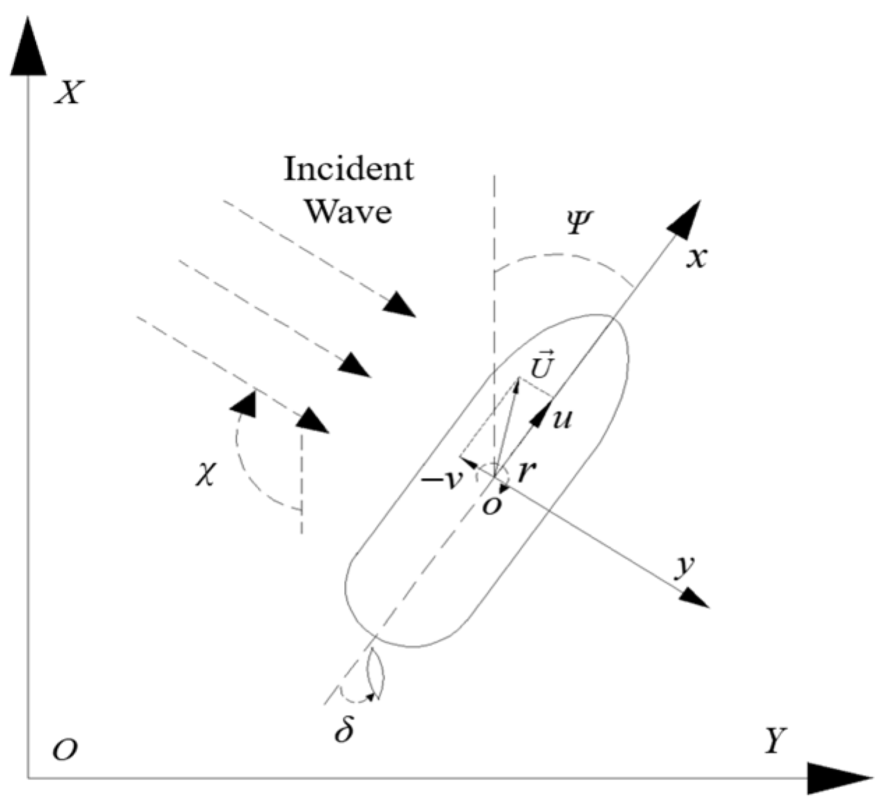
3.1. Coordinate Systems

Two right-handed coordinate systems are considered, as shown in Figure 2. The first coordinate system, O-XYZ is a fixed coordinate system in space, with positive Z pointing downward. The second coordinate system, o-xyz, moves with the ship’s maneuvering speed but does not oscillate with the ship. The oxy plane overlaps with the calm water surface, and its origin o is located at the intersection of the middle transverse section, middle longitudinal section, and the calm water surface. The ox, oy, and oz axes pointed to the bow, starboard, and vertically downward, respectively.

The space fixed coordinate system coincides with the ship moving coordinate system at the initial moment and have the following relationships:

$$\{\begin{array}{l}X=x\mathit{cos}\Psi (t)-y\mathit{sin}\Psi (t)+X_0(t)\\ Y=x\mathit{sin}\Psi (t)+y\mathit{cos}\Psi (t)+Y_0(t)\\ Z=z\end{array},$$

(1)

where Ψ is the heading angle, which is the included angle between the OX axis and the ox axis’ positive direction, and (X₀, Y₀) is the coordinate of the origin of the ship’s moving coordinate system in the fixed space coordinate system, which is used to represent the ship’s spatial position at different times. The incident wave angle χ is the angle between the wave heading and the X axis of the fixed coordinate system. When χ = 0°, the incident wave propagates along the positive direction of the X axis and is positive clockwise. δ represents the rudder angle, which stipulates that the starboard is positive, and t denotes time.

3.2. Basic Equations of Ship Maneuvering Motion

The ship’s motion equation is established in the ship’s moving coordinate system. In the calculation of ship motion, it is assumed that the ship is a moving rigid body; its shape and internal mass distribution do not change with the motion. Its longitudinal velocity is u, transverse velocity is v, combined velocity is $U=\sqrt{u^2+v^2}$, and yaw angular velocity is r. The basic equation of ship maneuvering motion is governed via the following equations:

$$\begin{array}{l}m(\dot{u}-vr-x_G{r}^2)=F_x\\ m(\dot{v}+ur+x_G\dot{r})=F_y\\ I_{zz}\dot{r}+m{x}_G(\dot{v}+ur)=M_z\end{array},$$

(2)

where m represents the ship’s mass, I_zz represents the moment of inertia around the Z-axis, x_G is the longitudinal coordinate of the center of gravity, and F_x, F_y, and M_z are the hydrodynamic forces and moment suffered by the ship, respectively. In maneuvering, the hydrodynamic force acting on the hull comprises inertial and non-inertial forces. In this study, the hydrodynamic forces and moment can be expressed by:

$$\begin{array}{l}{F}_x=-m_x\dot{u}+m_{y}vr+X_H+X_R+X_P+X_W\\ F_y=-m_y\dot{v}-m_{x}ur+Y_H+Y_R+Y_W\\ M_z=-J_{zz}\dot{r}+N_H+N_R+N_W\end{array},$$

(3)

where m_x and m_y are the corresponding added masses, and J_zz is the added moment of inertia. X_P, X_R, and X_H represent the longitudinal low-frequency hydrodynamic forces on the propeller, rudder, and hull, respectively. X_W denotes the surge wave drift force. The lateral force caused by propeller rotation and its torque on the center of gravity are ignored. Combining Equations (2) and (3), a new equation of ship motion can be obtained:

$$\begin{array}{l}(m+m_x)\dot{u}-(m+m_y)vr-m{x}_G{r}^2=X_H+X_R+X_P+X_W\\ (m+m_y)\dot{v}+(m+m_x)ur+m{x}_G\dot{r}=Y_H+Y_R+Y_W\\ (I_{zz}+J_{zz}+m{x}_G{}^2)\dot{r}+m{x}_G(\dot{v}+ur)=N_H+N_R+N_W\end{array}.$$

(4)

3.3. Hydrodynamic Forces Acting on Ship Hull

The hydrodynamic forces acting on the ship hull are expressed as follows:

$$\begin{array}{l}{X}_H=(\raisebox{1ex}{$1$}\!\left/ \!\raisebox{-1ex}{$2$}\right.)\rho L_{PP}d{U}^2{X^{\prime }}_H(v^{\prime },r^{\prime })\\ Y_H=(\raisebox{1ex}{$1$}\!\left/ \!\raisebox{-1ex}{$2$}\right.)\rho L_{PP}d{U}^2{Y^{\prime }}_H(v^{\prime },r^{\prime })\\ N_H=(\raisebox{1ex}{$1$}\!\left/ \!\raisebox{-1ex}{$2$}\right.)\rho L^2{}_{PP}d{U}^2{N^{\prime }}_H(v^{\prime },r^{\prime })\end{array},$$

(5)

where L_PP is the ship length between perpendiculars. v’ and r’ denotes the non-dimensional lateral velocity and yaw rate defined via v/U and rL_PP/U, respectively. X’_H, Y’_H, and N’_H are expressed as follows:

$$\begin{array}{l}{X^{\prime }}_H(v^{\prime },r^{\prime })=-{R^{\prime }}_0+{X^{\prime }}_{vv}{v^{\prime }}^2+{X^{\prime }}_{vr}{v}^{\prime }{r}^{\prime }+{X^{\prime }}_{rr}{r^{\prime }}^2+{X^{\prime }}_{vvvv}{v^{\prime }}^4\\ {Y^{\prime }}_H(v^{\prime },r^{\prime })={Y^{\prime }}_v{v}^{\prime }+{Y^{\prime }}_r{r}^{\prime }+{Y^{\prime }}_{vvv}{v^{\prime }}^3+{Y^{\prime }}_{vvr}{v^{\prime }}^2{r}^{\prime }+{Y^{\prime }}_{vrr}{v}^{\prime }{r^{\prime }}^2+{Y^{\prime }}_{rrr}{r^{\prime }}^3\\ {N^{\prime }}_H(v^{\prime },r^{\prime })={N^{\prime }}_v{v}^{\prime }+{N^{\prime }}_r{r}^{\prime }+{N^{\prime }}_{vvv}{v^{\prime }}^3+{N^{\prime }}_{vvr}{v^{\prime }}^2{r}^{\prime }+{N^{\prime }}_{vrr}{v}^{\prime }{r^{\prime }}^2+{N^{\prime }}_{rrr}{r^{\prime }}^3\end{array},$$

(6)

where R’₀ represents the resistance coefficient, and X’_vv, X’_vr, X’_rr, X’_vvvv, Y’_v, Y’_r, N’_v, N’_r, etc., are termed the non-dimensional hydrodynamic derivatives. Compared with the other hydrodynamic derivatives, Y’_H and N’_H calculated via the 1st and 3rd order polynomial functions of v’ and r’ have better estimation accuracy.

3.4. Hydrodynamic Force Due to Propeller

The hydrodynamic force due to the propeller X_p is expressed as:

$$X_P=(1-t_p)T,$$

(7)

where t_p is the thrust deduction fraction and is assumed to be constant. T is the propeller thrust and is expressed as follows:

$$T=\rho n_P{}^2{D}_p{}^4{K}_T(J_P),$$

(8)

where ρ, K_T, D_p, and n_p are the water density, thrust coefficient, propeller diameter, and propeller revolution, respectively. K_T is expressed via the propeller advance ratio J_P:

$$K_T(J_P)=k_2{J}_p{}^2+k_1{J}_p+k_0,$$

(9)

J_P is expressed as:

$$J_p=\frac{u(1-w_p)}{n_p{D}_p},$$

(10)

where w_p is the wake coefficient at the propeller, which is usually expressed via the wake coefficient w_p0 in a straight motion. The Yasukawa et al. [27] model is adopted as follows:

$$(1-w_p)/(1-w_{p0})=1+\left\{1-\mathit{exp}(-C_1\left|{\beta }_p\right|)\right\}\left(C_2-1\right),$$

(11)

where C₁ and C₂ are the experimental constants representing the wave characteristics during maneuvering obtained via Yasukawa et al. [27]. β_p is the geometrical inflow angle to the propeller in maneuvering motion and is calculated as follows:

$${\beta }_P=\beta -{x^{\prime }}_p{r}^{\prime }={\mathit{tan}}^{-1}(-v/u)-{x^{\prime }}_p{r}^{\prime }.$$

(12)

where x’_p is the non-dimensional longitudinal coordinate of the propeller by L_PP and β is the drift angle.

3.5. Hydrodynamic Forces by Steering

The rudder forces and moment are expressed as:

$$\begin{array}{l}{X}_R=-(1-t_R)F_N\mathit{sin}\delta \\ Y_R=-(1+{\alpha }_H)F_N\mathit{cos}\delta \\ N_R=-(x_R+{\alpha }_H{x}_H)F_N\mathit{cos}\delta \end{array},$$

(13)

where F_N, δ, and x_R are the rudder normal force, rudder angle, and longitudinal position of the rudder, respectively. α_H, t_R, and x_H are the rudder force increase factor, steering resistance deduction factor, and the position of an additional lateral force component, respectively.

Rudder normal force F_N is expressed as:

$$F_N=(1/2)\rho A_R{U}^2{}_R{f}_{\alpha }\mathit{sin}{\alpha }_R,$$

(14)

where A_R and f_α represent the profile area of the movable part of the rudder and rudder lift gradient coefficient, respectively. U_R and α_R represent the resultant rudder inflow velocity and the inflow angle, respectively, and are expressed as:

$$U_R=\sqrt{u^2{}_R+v^2{}_R},$$

(15)

$${\alpha }_R=\delta -{\mathit{tan}}^{-1}\left(\frac{v_R}{u_R}\right)\simeq \delta -\frac{v_R}{u_R},$$

(16)

Here, δ is the rudder angle. u_R and v_R represent the longitudinal and lateral inflow velocity components to the rudder, respectively.

$$u_R=\epsilon u\left(1-w_p\right)\sqrt{\eta {\left\{1+\kappa \left(\sqrt{1+\frac{8K_T}{\pi J_p^2}}-1\right)\right\}}^2+\left(1-\eta \right)},$$

(17)

$$v_R=U{\gamma }_R{\beta }_R,$$

(18)

$${\beta }_R=\beta -{l^{\prime }}_R{r}^{\prime }.$$

(19)

Here, ε, l’_R, κ, and γ_R represent the ratio of wake fraction at the rudder position to that at the propeller position, the effective non-dimensional longitudinal coordinate of the rudder position, an experimental constant, and the flow straightening coefficient, respectively. η = D_p/H_R, where H_R is the rudder span length. The relevant coefficient values are obtained via Yasukawa et al. [27].

4. Wave-Induced Motion

4.1. Boundary Value Problem and Wave Drift Loads

Based on the potential flow theory, incompressible and inviscid water is assumed, and the flow is irrotational. Thus, the water motion can be described by the velocity potential $\Theta$, which satisfies the Laplace equation and boundary value conditions. The boundary value problem can be linearized by decomposing the velocity potential $\Theta$, including the base velocity potential Φ_b, the steady wave flow velocity potential, ϕ, and the unsteady wave flow velocity potential φ.

$$\Theta ={\Phi }_b+\varphi +\phi =-ux-\mathrm{vy}+\Phi +\varphi +{\phi }_I+{\phi }_d,$$

(20)

The base velocity potential Φ_b can be divided into the incoming flow velocity potential and the DB flow velocity potential, Φ. The unsteady wave flow potential φ can be divided into the disturbed potential φ_d and incident potential φ_I. Wave elevation can also be divided into steady, disturbed, and incident terms (${\zeta }_S$,${\zeta }_d$, and ${\zeta }_I$), respectively.

$$\zeta ={\zeta }_S+{\zeta }_d+{\zeta }_I,$$

(21)

Only the unsteady flow is discussed in this paper; the steady wave flow velocity potential and the steady wave elevation are ignored. Based on the DB assumption, the velocity potential Φ satisfies the following boundary value problem:

$$\{\begin{array}{l}{\nabla }^2\Phi =0\\ \frac{\partial \Phi }{\partial n}=\overrightarrow{M}\times \overrightarrow{n} \left(on S_H\right)\\ \frac{\partial \Phi }{\partial z}=0 \left(on S_F\right)\\ \Phi =0\left(\sqrt{x^2+y^2+z^2}\to \infty \right)\end{array},$$

(22)

where $\overrightarrow{M}=u\overrightarrow{i}+v\overrightarrow{j}+0\overrightarrow{k}$, S_H is the mean wet surface of the hull, and S_F is the undisturbed free surface.

After the velocity potential Φ is solved, the m_j terms can be expressed as follows:

$$\begin{array}{l}\left(m_1,m_2,m_3\right)=-\left(\overrightarrow{n}\cdot \nabla \right)\overrightarrow{W}\\ \left(m_4,m_5,m_6\right)=-\left(\overrightarrow{n}\cdot \nabla \right)\left[\overrightarrow{r}\times \overrightarrow{W}\right]\end{array}$$

(23)

where $\overrightarrow{W}=\left(\frac{\partial \Phi }{\partial x}-u\right)\overrightarrow{i}+\left(\frac{\partial \Phi }{\partial y}-v\right)\overrightarrow{j}+\frac{\partial \Phi }{\partial z}\overrightarrow{k}$ and $\overrightarrow{r}$ denotes the distance between the fluid point and mass centroid of the ship.

The linearized incident velocity potential in deep water is known analytically, as follows:

$${\phi }_I=A\frac{g}{\omega }{e}^{kz}\mathit{sin}\left\{k\left[x\mathit{cos}\left(\chi -\Psi \right)+y\mathit{sin}\left(\chi -\Psi \right)+X_0\mathit{cos}\chi +Y_0\mathit{sin}\chi \right]-\omega t\right\},$$

(24)

where A, k, g, and ω denote the wave amplitude, wave number, acceleration of gravity, and frequency of the incident wave, respectively. Ψ and χ are the heading and incident angles of the wave.

The damping zone is used to deal with the distant radiation condition of the ship with a forward speed problem. Thus, the boundary value problem of the disturbed potential is:

$$\{\begin{array}{l}{\nabla }^2{\phi }_d=0\\ \frac{\partial {\phi }_d}{\partial n}=-\frac{\partial {\phi }_I}{\partial n}+{\displaystyle \sum _{j=1}^6\left(\frac{\partial {\eta }_j}{\partial t}{n}_j+{\eta }_j{m}_j\right)} \left(on{ \mathrm{S}}_H\right)\\ \left[\frac{\partial }{\partial t}+\left(\nabla \Phi -\overrightarrow{M}\right)\cdot \nabla \right] {\zeta }_d= \frac{\partial {\phi }_d}{\partial z} + \frac{{\partial }^2\Phi }{\partial z^2} {\zeta }_d-\mu {\zeta }_d+f_1 \left(on{ \mathrm{S}}_{\mathrm{F}}\right)\\ \left[\frac{\partial }{\partial t}+\left(\nabla \Phi -\overrightarrow{M}\right)\cdot \nabla \right]{\phi }_d =-g{\zeta }_d-\mu {\phi }_d+f_2 \left(on{ \mathrm{S}}_{\mathrm{F}}\right)\\ {{\phi }_d|}_{t=0}=0,{\frac{\partial {\phi }_d}{\partial n}|}_{t=0}=0 \left(The initial conditions\right)\end{array},$$

(25)

Here $\left(n_1,n_2,n_3\right)=n_j, \left(n_4,n_5,n_6\right)=\overrightarrow{r}\times n_j$, and ${\eta }_j(j=1-6)$ are the 6-DOF motion displacements of the ship. $\mu =3{\mu }_0{(l-l_0)}^2/L^2-2{\mu }_0{(l-l_0)}^3/L^3$,$f_1=\left(\frac{{\partial }^2\Phi }{\partial z^2}-\nabla \Phi \cdot \nabla \right){\zeta }_I$ and $f_2=-\nabla \Phi \cdot \nabla {\phi }_I$, where l₀, L, and ${\mu }_0$ are the initial edge, damping length, and the damping intensity of the damping zone, respectively.

When the unsteady disturbed potential is solved, the first-order wave force can be obtained via integrating the pressure on the wetted surface of the ship, as follows:

$${\overrightarrow{F}}^{(1)}=-\rho \underset{s_H}{\mathsf{\iint }}\left[\frac{\partial \phi }{\partial t}+\overrightarrow{W}\cdot \nabla \phi \right]{\overrightarrow{n}}^{(0)}ds.,$$

(26)

We can also solve the restoring force via the restoring force coefficient matrix. Then, the motion of the ship can be obtained from the wave-induced 6-DOF motion equations, as follows:

$${\displaystyle \sum _{j=1}^6{m}_{ij}{\ddot{\zeta }}_j(t)}=F_i, i=1,2,\mathrm{\dots },6,$$

(27)

Here (${\zeta }_1$, ${\zeta }_2$, ${\zeta }_3$) and (${\zeta }_4$, ${\zeta }_5$, ${\zeta }_6$) represent the translation and rotational displacements of the ship, respectively. m_ij represents the elements of the inertial matrix for the hull. F_i denotes the first-order wave forces, including restoring, radiation, diffraction, and Froude–Kriloff forces. The first-order wave forces are also referred to as the wave frequency hydrodynamic forces.

The wave drift loads can be obtained via pressure integration on the body surface. We adopted the formulation of the pressure integration provided by Chen et al. [28] as follows:

$$\begin{array}{ll}{\overrightarrow{F}}^{(2)}& ={\underset{WL}{\int }\frac{1}{2}\rho g\left[\zeta -{\delta }_3\right]}^2{\overrightarrow{n}}^{(0)}dL+\rho \underset{WL}{\int }\left[\overrightarrow{W}\cdot \nabla \Phi -\frac{1}{2}{(\nabla \Phi )}^2\right]\left[\zeta -{\delta }_3\right]{\overrightarrow{n}}^{(1)}dL\\ & +\rho \underset{WL}{\int }\overrightarrow{\delta }\cdot \nabla \left[\overrightarrow{W}\cdot \nabla \Phi -\frac{1}{2}{(\nabla \Phi )}^2\right]\left[\zeta -{\delta }_3\right]{\overrightarrow{n}}^{(0)}dL+\rho \underset{S_H}{\iint }\left[\overrightarrow{W}\cdot \nabla \Phi -\frac{1}{2}{(\nabla \Phi )}^2-gz\right]{\overrightarrow{n}}^{(2)}ds\\ & -\rho \underset{S_H}{\iint }\frac{1}{2}\nabla {\phi }^2{\overrightarrow{n}}^{(0)}ds-\rho \underset{S_H}{\iint }\overrightarrow{\delta }\cdot \nabla \left[\frac{\partial \phi }{\partial t}+\overrightarrow{W}\cdot \nabla \phi \right]{\overrightarrow{n}}^{(0)}ds\\ & -\rho \underset{S_H}{\iint }\left[g{\delta }_3+\frac{\partial \phi }{\partial t}+\overrightarrow{W}\cdot \nabla \phi \right]{\overrightarrow{n}}^{(1)}ds+\rho \underset{S_H}{\iint }\overrightarrow{\delta }\cdot \nabla \left[\overrightarrow{W}\cdot \nabla \Phi -\frac{1}{2}{(\nabla \Phi )}^2\right]{\overrightarrow{n}}^{(1)}ds\end{array}$$

(28)

$$\begin{array}{ll}{\overrightarrow{M}}^{(2)}& ={\underset{WL}{\int }\frac{1}{2}\rho g\left[\zeta -{\delta }_3\right]}^2(\overrightarrow{r}\times {\overrightarrow{n}}^{(0)})dL+\rho \underset{WL}{\int }\left[\overrightarrow{W}\cdot \nabla \Phi -\frac{1}{2}{(\nabla \Phi )}^2\right]\left[\zeta -{\delta }_3\right](\overrightarrow{r}\times {\overrightarrow{n}}^{(1)})dL\\ & +\rho \underset{WL}{\int }\overrightarrow{\delta }\cdot \nabla \left[\overrightarrow{W}\cdot \nabla \Phi -\frac{1}{2}{(\nabla \Phi )}^2\right]\left[\zeta -{\delta }_3\right](\overrightarrow{r}\times {\overrightarrow{n}}^{(0)})dL\\ & +\rho \underset{S_H}{\iint }\left[\overrightarrow{W}\cdot \nabla \Phi -\frac{1}{2}{(\nabla \Phi )}^2-gz\right](\overrightarrow{r}\times {\overrightarrow{n}}^{(2)}+{\overrightarrow{r}}^{(2)}\times {\overrightarrow{n}}^{(0)})ds\\ & -\rho \underset{S_H}{\iint }\frac{1}{2}\nabla {\phi }^2(\overrightarrow{r}\times {\overrightarrow{n}}^{(0)})ds-\rho \underset{S_H}{\iint }\overrightarrow{\delta }\cdot \nabla \left[\frac{\partial \phi }{\partial t}+\overrightarrow{W}\cdot \nabla \phi \right](\overrightarrow{r}\times {\overrightarrow{n}}^{(0)})ds\\ & -\rho \underset{S_H}{\iint }\left[g{\delta }_3+\frac{\partial \phi }{\partial t}+\overrightarrow{W}\cdot \nabla \phi \right](\overrightarrow{r}\times {\overrightarrow{n}}^{(1)})ds+\rho \underset{S_H}{\iint }\overrightarrow{\delta }\cdot \nabla \left[\overrightarrow{W}\cdot \nabla \Phi -\frac{1}{2}{(\nabla \Phi )}^2\right](\overrightarrow{r}\times {\overrightarrow{n}}^{(1)})ds\end{array}$$

(29)

Here, $\overrightarrow{\delta }=({\delta }_1,{\delta }_2,{\delta }_3)$ represents the resultant displacement at any point of the ship and ${\overrightarrow{n}}^{(0)}$ represents the normal vector when the ship is stationary. Here ${\overrightarrow{n}}^{(1)}=H^{(1)}\overrightarrow{n}, {\overrightarrow{n}}^{(2)}=H^{(2)}\overrightarrow{n}$, ${\overrightarrow{r}}^{(2)}=H^{(1)}\overrightarrow{r}$,

$$H^{(1)}=\left\{\begin{array}{ccc}0& -{\eta }_6& {\eta }_5\\ {\eta }_6& 0& -{\eta }_4\\ -{\eta }_5& {\eta }_4& 0\end{array}\right\}, H^{(2)}=-\frac{1}{2}\left\{\begin{array}{ccc}{\eta }_5{}^2+{\eta }_6{}^2& 0& 0\\ -2{\eta }_4{\eta }_5& {\eta }_4{}^2+{\eta }_6{}^2& 0\\ -2{\eta }_4{\eta }_6& -2{\eta }_5{\eta }_6& {\eta }_4{}^2+{\eta }_5{}^2\end{array}\right\}.$$

4.2. Taylor Expansion Boundary Element Method (TEBEM)

Given the low calculation accuracy of the constant surface element method for solving the sharp corner of the object surface and since the high-order boundary element method cannot directly calculate the high-order derivative of the velocity potential at the corner, the TEBEM is used to solve the disturbance velocity potential and its higher-order derivatives, which can effectively improve the calculation accuracy. The TEBEM is based on the source and dipole mixed distribution model. The potential functions φ and Green’s function 1/r (p, q) are the basic solutions of the Laplace equation. r represents the distance between the field point p and the source point q. When the field point p is in the fluid domain, the following formula can be obtained using Green’s third formula for φ and 1/r (p, q):

$$4\pi \phi (p,t)=\underset{S}{\iint }\left[\frac{\partial \phi (q,t)}{\partial n_q}\frac{1}{r(p,q)}-\phi (q,t)\frac{\partial }{\partial n_q}\left(\frac{1}{r(p,q)}\right)\right]d{S}_q,$$

(30)

Here, the unit normal vector n_q points to the outer part of the fluid domain; S represents the boundary of the fluid domain and can be discretized into N small triangular or quadrilateral elements. The average value of each element node is taken as the center and the discrete format is as follows:

$$4\pi \phi (p,t)={\displaystyle \sum _{i=1}^N\underset{\Delta S_i}{\iint }\left[\frac{\partial \phi (q,t)}{\partial n_q}\frac{1}{r(p,q)}-\phi (q,t)\frac{\partial }{\partial n_q}\left(\frac{1}{r(p,q)}\right)\right]d{S}_q},$$

(31)

When the field point P approaches the boundary of the fluid domain along the negative direction of the normal vector, the boundary integral can be obtained as follows:

$$2\pi \phi (p,t)+{\displaystyle \sum _{i=1}^N\underset{\Delta S_i}{\iint }\left[\phi (p,t)\frac{\partial }{\partial n_q}(\frac{1}{r(p,q)})\right]d{S}_q}={\displaystyle \sum _{i=1}^N\underset{\Delta S_i}{\iint }\left[\frac{\partial \phi (q,t)}{\partial n_q}(\frac{1}{r(p,q)})\right]d{S}_q},$$

(32)

Here N represents the number of panels at the surface of the ship and the free surface.

For the dipole strength in Equation (32), the Taylor expansion is performed in the local coordinate system of each panel, and the first-order derivative term is retained as follows:

$$\phi (q)=\phi \left(q_0\right)+{\phi }_{\xi }\left(q_0\right)\overline{\xi }+{\phi }_{\eta }\left(q_0\right)\overline{\eta },$$

(33)

where $\overline{\eta }$ and $\overline{\xi }$ are the local coordinates of the source point, as shown in Figure 3.

The new boundary integral can be obtained via substituting Equation (33) into Equation (32) as:

$$\begin{array}{l}2\pi \phi (p,t)+{\displaystyle \sum _{i=1}^N\phi (q_0,t)}\underset{\Delta S_i}{\iint }\frac{\partial }{\partial n_q}(\frac{1}{r(p,q)})d{S}_q+{\displaystyle \sum _{i=1}^N\frac{\partial \phi (q_0,t)}{\partial \overline{\xi }}}\underset{\Delta S_i}{\iint }\overline{\xi }\frac{\partial }{\partial n_q}(\frac{1}{r(p,q)})d{S}_q\\ +{\displaystyle \sum _{i=1}^N\frac{\partial \phi (q_0,t)}{\partial \overline{\eta }}\underset{\Delta S_i}{\iint }\overline{\eta }\frac{\partial }{\partial n_q}(\frac{1}{r(p,q)})d{S}_q}={\displaystyle \sum _{i=1}^N\frac{\partial \phi (q_0,t)}{\partial nq}}\underset{\Delta S_i}{\iint }\frac{1}{r(p,q)}d{S}_q\end{array},$$

(34)

To solve Equation (34), we need to add a new boundary integral equation. The first-order derivatives of the potential at the field point are considered, along with the two mutually orthogonal tangential directions. The supplementary equations are:

$$\begin{array}{l}2\pi \frac{\partial \phi (p,t)}{\partial \overline{x}}+{\displaystyle \sum _{i=1}^N\phi (q_0,t)}\underset{\Delta S_i}{\iint }\frac{{\partial }^2}{\partial \overline{x}\partial n_q}(\frac{1}{r(p,q)})d{S}_q+{\displaystyle \sum _{i=1}^N\frac{\partial \phi (q_0,t)}{\partial \overline{\xi }}}\underset{\Delta S_i}{\iint }\overline{\xi }\frac{{\partial }^2}{\partial \overline{x}\partial n_q}(\frac{1}{r(p,q)})d{S}_q\\ +{\displaystyle \sum _{i=1}^N\frac{\partial \phi (q_0,t)}{\partial \overline{\eta }}\underset{\Delta S_i}{\iint }\overline{\eta }\frac{{\partial }^2}{\partial \overline{x}\partial n_q}(\frac{1}{r(p,q)})d{S}_q}={\displaystyle \sum _{i=1}^N\frac{\partial \phi (q_0,t)}{\partial n_q}}\underset{\Delta S_i}{\iint }\frac{\partial }{\partial \overline{x}}\frac{1}{r(p,q)}d{S}_q\end{array},$$

(35)

$$\begin{array}{l}2\pi \frac{\partial \phi (p,t)}{\partial \overline{y}}+{\displaystyle \sum _{i=1}^N\phi (q_0,t)}\underset{\Delta S_i}{\iint }\frac{{\partial }^2}{\partial \overline{y}\partial n_q}(\frac{1}{r(p,q)})d{S}_q+{\displaystyle \sum _{i=1}^N\frac{\partial \phi (q_0,t)}{\partial \overline{\xi }}}\underset{\Delta S_i}{\iint }\overline{\xi }\frac{{\partial }^2}{\partial \overline{y}\partial n_q}(\frac{1}{r(p,q)})d{S}_q\\ +{\displaystyle \sum _{i=1}^N\frac{\partial \phi (q_0,t)}{\partial \overline{\eta }}\underset{\Delta S_i}{\iint }\overline{\eta }\frac{{\partial }^2}{\partial \overline{y}\partial n_q}(\frac{1}{r(p,q)})d{S}_q}={\displaystyle \sum _{i=1}^N\frac{\partial \phi (q_0,t)}{\partial n_q}}\underset{\Delta S_i}{\iint }\frac{\partial }{\partial \overline{y}}\frac{1}{r(p,q)}d{S}_q\end{array}.$$

(36)

Finally, we can obtain the dipole strength and its first-order derivatives via solving Equations (34)–(36). All the influencing coefficients for the solution process can be found in Duan et al. [26].

5. Numerical Results and Discussions

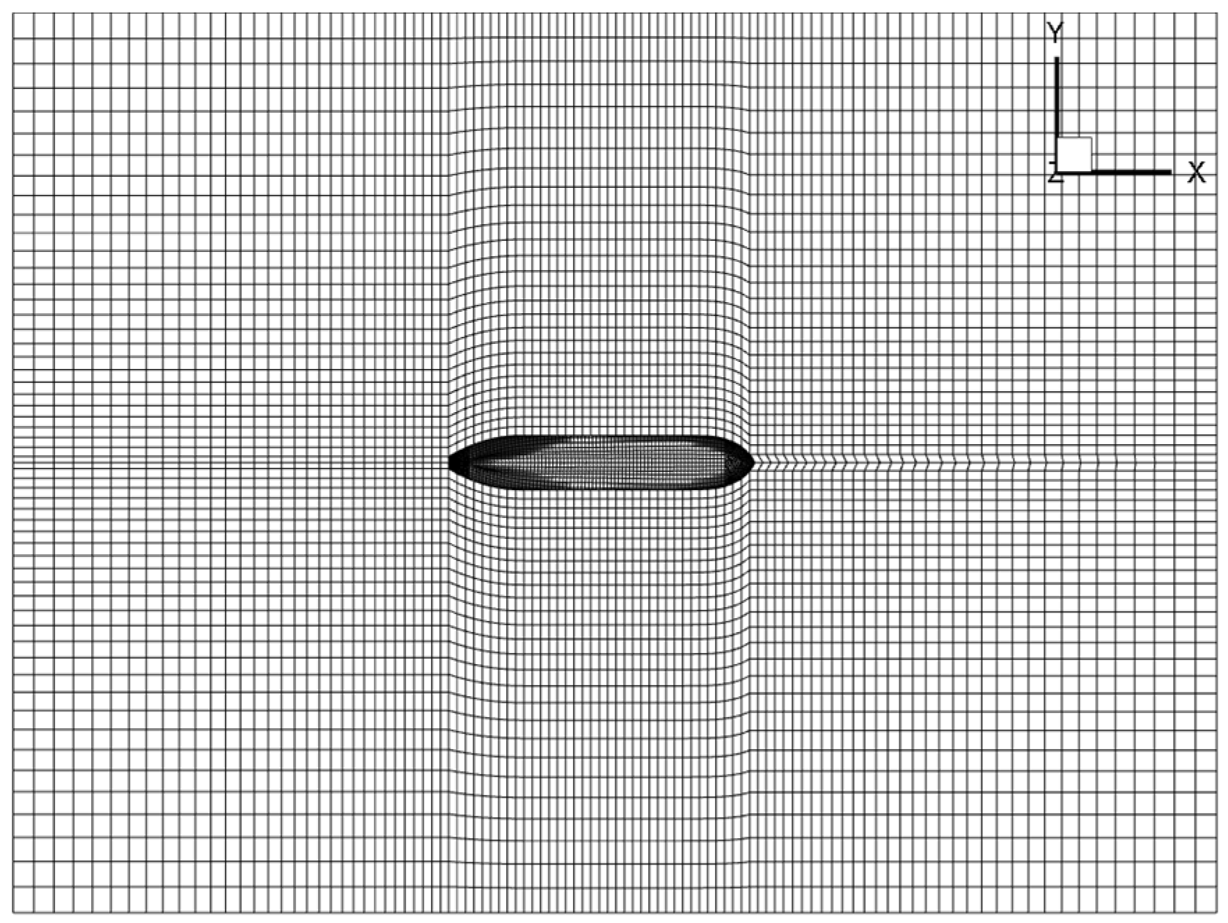
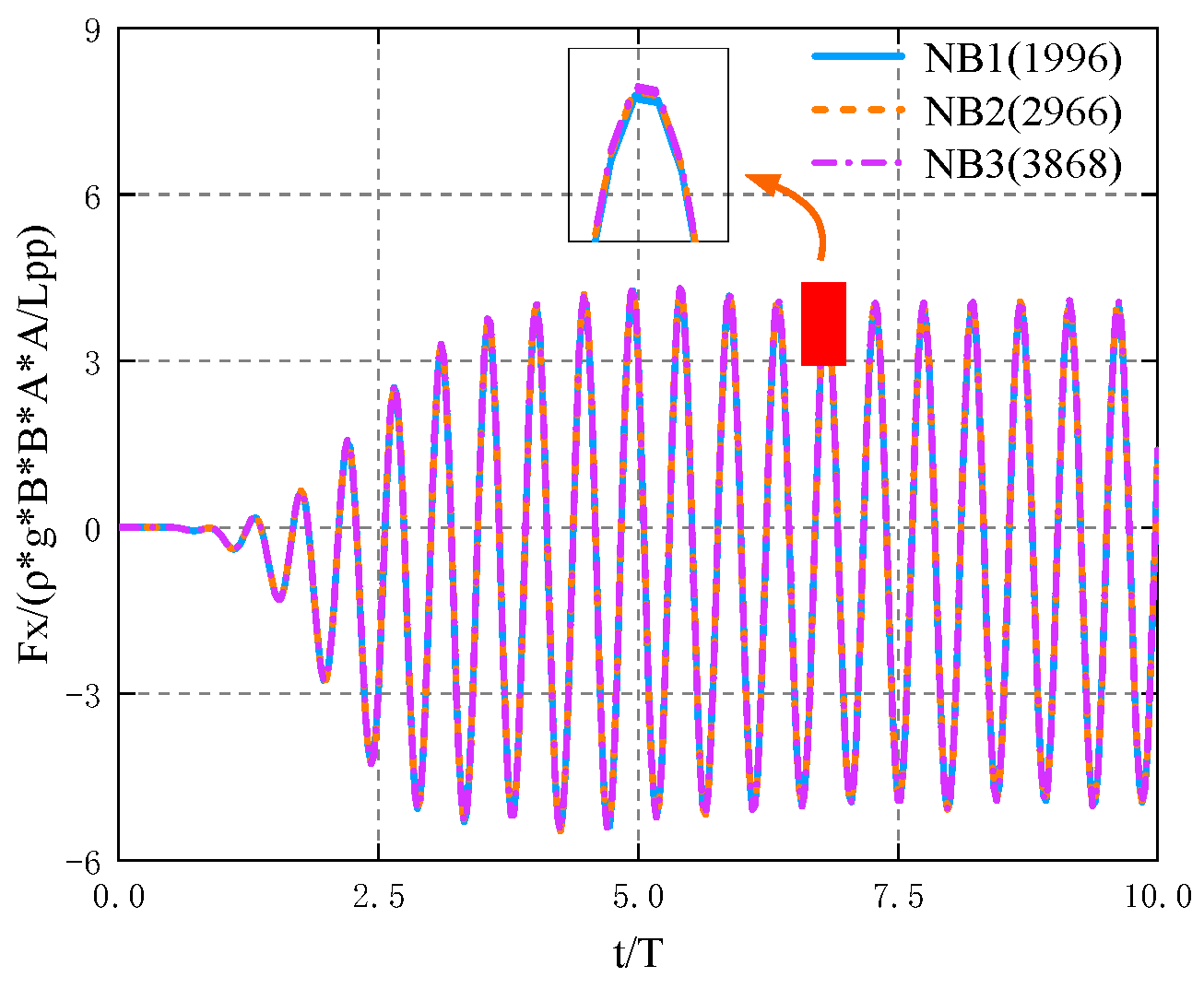
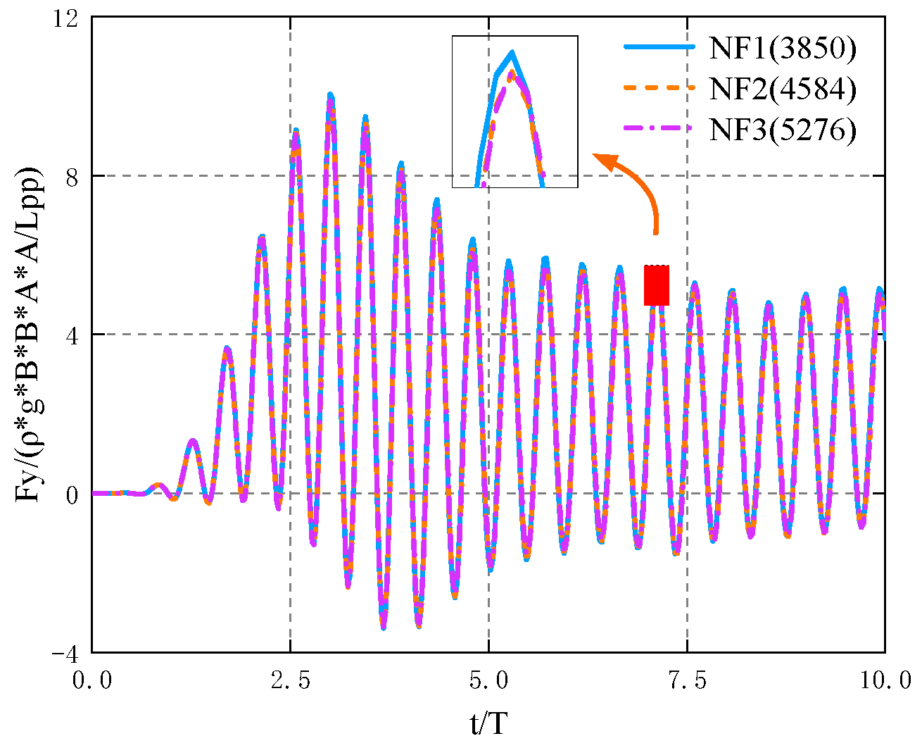
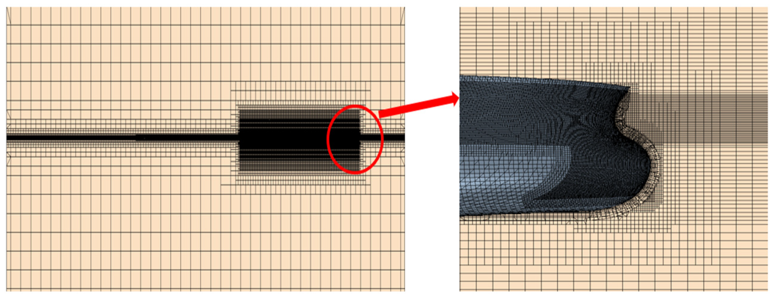
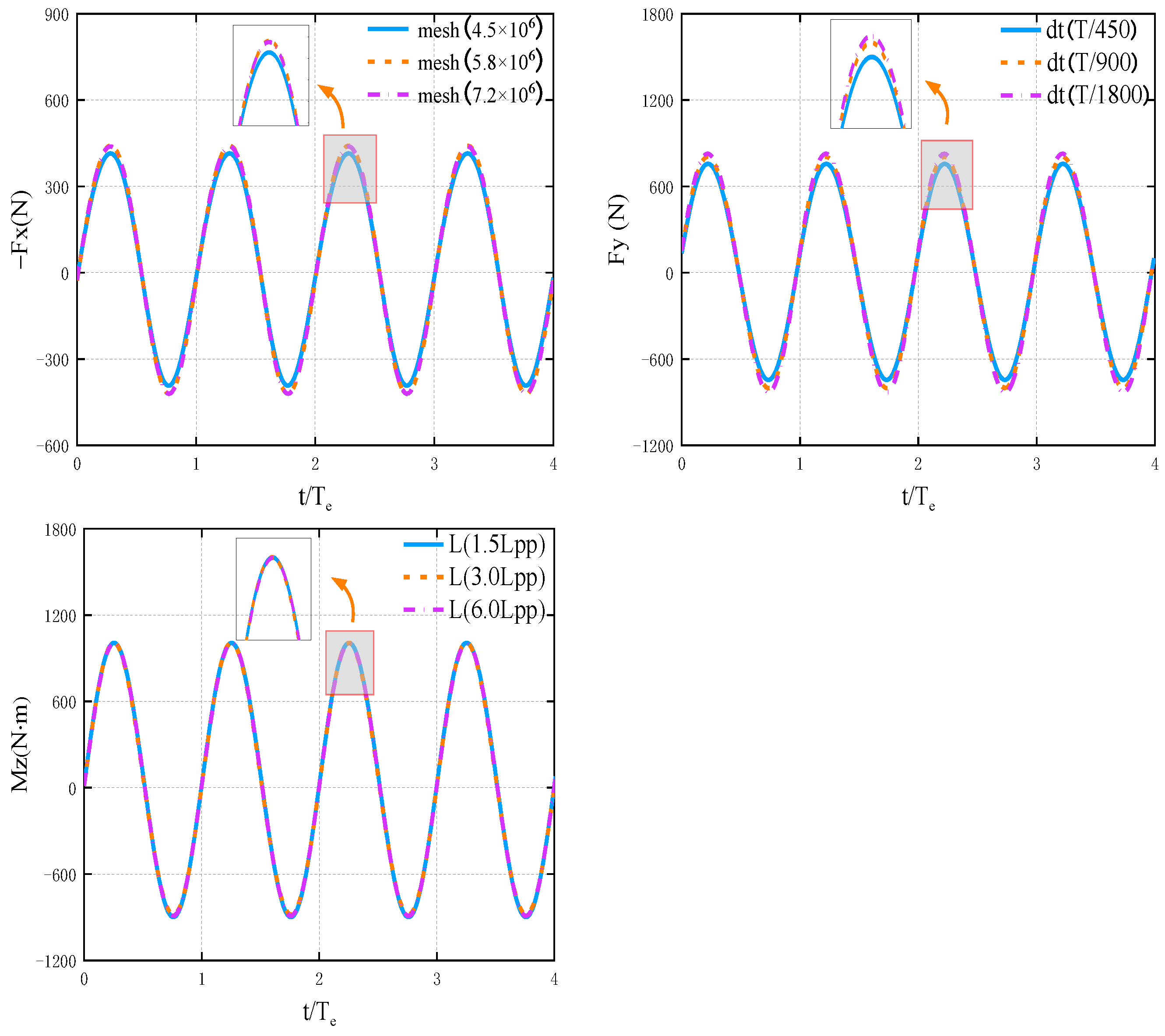
5.1. Convergence Analysis

The KVLCC2 ship model is used to calculate the wave drift loads of ships with drift angles in oblique waves and the turning motion in regular waves. The main parameters of the KVLCC2 ship model are shown in

Table 1. Main parameters of the KVLCC2 ship.

	Full Scale	Model
Scale	1.00	1/45.7
Ship length, LPP (m)	320.0	7.00
Breadth, B (m)	58.0	1.27
Draught, d (m)	20.8	0.455
Displacement, ∇ (m3)	312,600	3.27
Block coefficient, Cb	0.81	0.81
Longitudinal coordinate of the center of gravity of the ship, xG (m)	11.2	0.25
Radius of gyration, kxx, kyy, kzz (m)	19.33, 76.78,76.78	0.423, 1.68, 1.68
Propeller diameter, Dp (m)	9.86	0.216
Rudder height, HR (m)	15.80	0.345
Rudder area, AR (m2)	112.5	0.0539

.

The convergence analysis is conducted to verify the reliability of the numerical results. Based on the TEBEM, the wave drift loads of the KVLCC2 model are calculated with wave height H = 0.02 L_PP, wavelength λ = 1.0 L_PP, wave heading χ = 120°, drift angle β = 0°, and U = 6.0 kn. Figure 4 is a grid diagram of the hull surface below the waterline. The bow and stern of the ship are triangular grids, and the rest are quadrilateral grids. Figure 5 is the grid diagram of the free surface. Since the damping region is around the computational domain, the grid becomes sparser the farther away from the ship’s surface. Four soft springs are added in the horizontal direction of the ship to prevent the divergence of numerical simulation results, as shown in Figure 6. The spring’s stiffness is chosen so that the natural period of planar motion is five times the highest wave period.

Firstly, we develop the convergence of the full-body surface panel numbers, where the panel numbers of the free surface and the time-step scales are NF = 4584 and dt = T/55, respectively, where T is the wave period. Figure 7 shows the surge wave drift force of the KVLCC2 ship under H = 0.02 L_PP, λ = 1.0 L_pp, χ =120°, β = 0°, and U = 6.0 kn. Good convergence is obtained for different panel numbers of the full-body surface (NB = 1996, 2966, and 3868). Subsequently, the convergence of the panel numbers of the free surface (NF = 3850, 4584, and 5276) is analyzed, where the panel numbers of the full-body surface and the time-step scales are NB = 2966 and dt = T/55, respectively. Figure 8 shows the sway wave drift force of the KVLCC2 ship under H = 0.02 L_PP, λ = 1.0 L_pp, χ = 120°, β = 0°, and U = 6.0 kn. The sway wave drift force has better convergence under different panel numbers of the free surface. Finally, the convergence of the time-step scales (dt = T/45, dt = T/55, and dt = T/65) is analyzed, where the panel numbers of the full-body surface and the panel numbers of the free surface are NB = 2966 and NF = 4584, respectively. Figure 9 shows the yaw wave drift moment of the KVLCC2 ship under H = 0.02 L_PP, λ = 1.0 L_PP, χ = 120°, β = 0°, and U = 6.0 kn. As shown in Figure 9, the yaw wave drift moment of the KVLCC2 ship converges well.

Therefore, comprehensively considering the overall calculation accuracy and efficiency, the panel numbers of the full-body and free surfaces are selected as 2966 and 4584, respectively, and the time-step scale is T/55 for the subsequent calculation.

To verify the accuracy of the TEBEM, the Computational Fluid Dynamic (CFD) method is also used to calculate the wave drift loads of the ship by the popular commercial program STAR-CCM+ (v15.04). The second-order wave drift load of the ship in waves can be obtained by subtracting the surge, sway, and yaw forces and moment of the ship in calm water from the surge, sway, and yaw forces and moment of the ship in waves. Similarly, the convergence of the computational domain mesh, time-step scales, and damping zone length is analyzed for the surge, sway, and yaw forces and moment of the ship in waves. Figure 10 and Figure 11 are grid diagrams of the longitudinal section and damping zone of the computational domain, respectively. We retain only the first-order and second-order results of the calculated wave drift loads. Therefore, Equation (37) is used to carry out the least square fitting, where ω represents wave frequency. Figure 12 shows the least square fitting of the wave drift loads of the KVLCC2 ship under H = 0.02 L_PP, λ = 1.0 L_PP, χ = 120°, β = 0°, and U = 6.0 kn.

$$y=a_0+a_1\mathit{cos}\omega t+b_1\mathit{sin}\omega t+a_2\mathit{cos}2\omega t+b_2\mathit{sin}2\omega t$$

(37)

Figure 13 shows the time history diagram of the surge, sway, and yaw wave drift forces and moment of the KVLCC2 ship under H = 0.02 L_PP, λ = 1.1 L_PP, χ = 120°, β = 0°, and U = 6.0 kn, which correspond to different grid numbers of the computational domain (4.5 × 10⁶, 5.8 × 10⁶, and 7.5 × 10⁶), time-step scales (T/450, T/900, and T/1800), and damping zone length (1.5 Lpp, 3.0 Lpp, and 6.0 Lpp), respectively. Compared with different model results, it is clear that the surge, sway, and yaw wave drift force, and moment of the KVLCC2 ship have better convergence. Considering the overall calculation accuracy and efficiency, the grid numbers of the computational domain, time-step scales, and damping zone length are selected as 5.8 × 10⁶, T/900, and 3.0 L_PP, respectively.

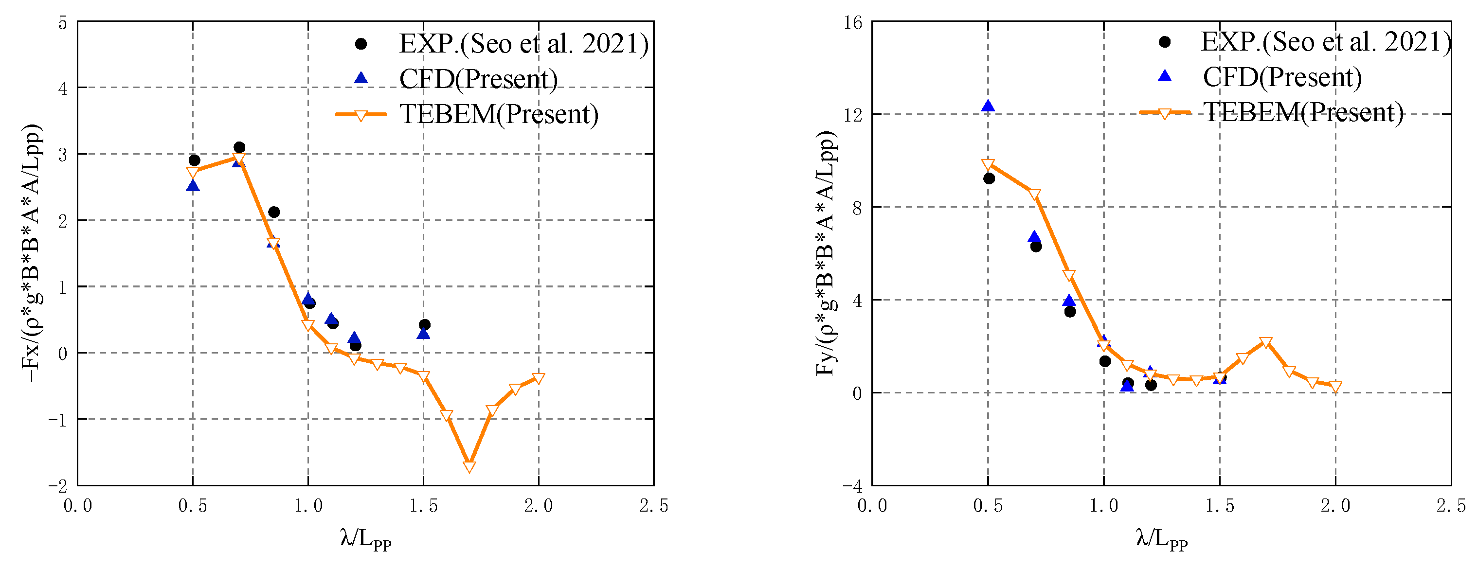
5.2. Wave Drift Loads Analysis of Ships with Zero Drift Angle in Oblique Waves

Since the wave drift loads play an important role in the ship’s turning motion, the wave drift loads and the 6-DOF motion of the KVLCC2 ship are calculated first via TEBEM and CFD method. Figure 14 shows the KVLCC2 ship’s RAO of 6-DOF motion under H = 0.02 L_PP, χ = 120°, β = 0°, and U = 6.0 kn. As shown in Figure 14, the computational results of CFD and TEBEM agree well with the experimental results of Seo et al. [29]. When λ/L_PP = 1.7, the roll motion significantly increases, indicating that the ship is near the roll resonance. However, the amplitude of roll resonance is obviously smaller than the experimental value, because only linearized viscous roll damping is considered at approximately 2% of the critical roll damping, which is not accurate enough for cases with non-zero speed.

Figure 15 shows the surge, sway, and yaw wave drift forces and moment of the KVLCC2 ship under H = 0.02 L_PP, χ = 120°, β = 0°, and U = 6.0 kn. The results of the TEBEM and CFD methods are also consistent with the trend of experimental values of Seo et al. [29]. The results calculated via TEBEM vary noticeably when λ/L_PP ≥ 1.5, due to the roll resonance motion. Vertical displacement ${\delta }_3$ is involved in Equations (28) and (29), which is the function of the roll motion displacement ${\eta }_4$, ${\delta }_3={\eta }_3+{\eta }_{4}y-{\eta }_{5}x$. For surge, sway, and yaw wave drift forces and moment, the accuracy of TEBEM can meet the requirements compared with the experimental values of Seo et al. [29].

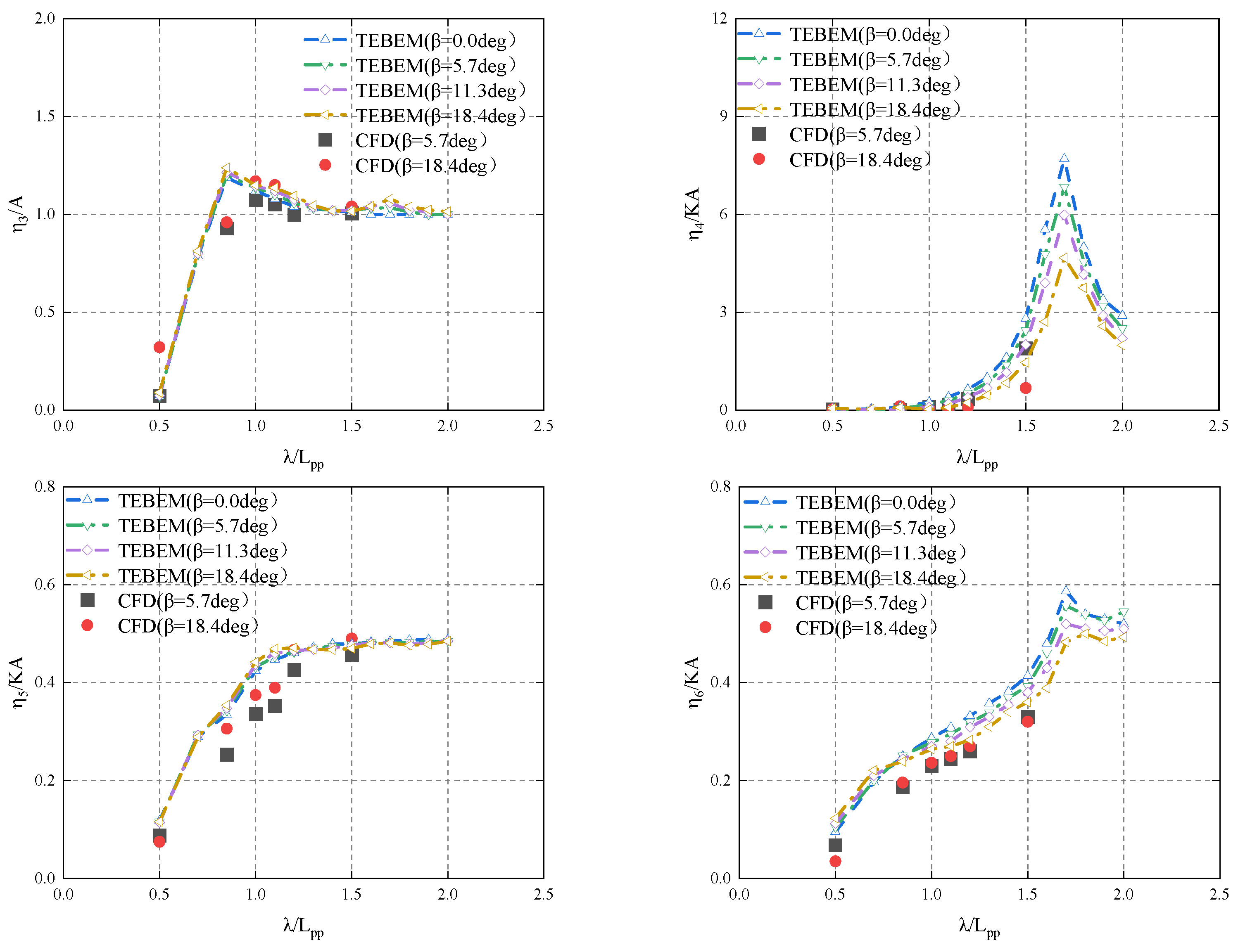
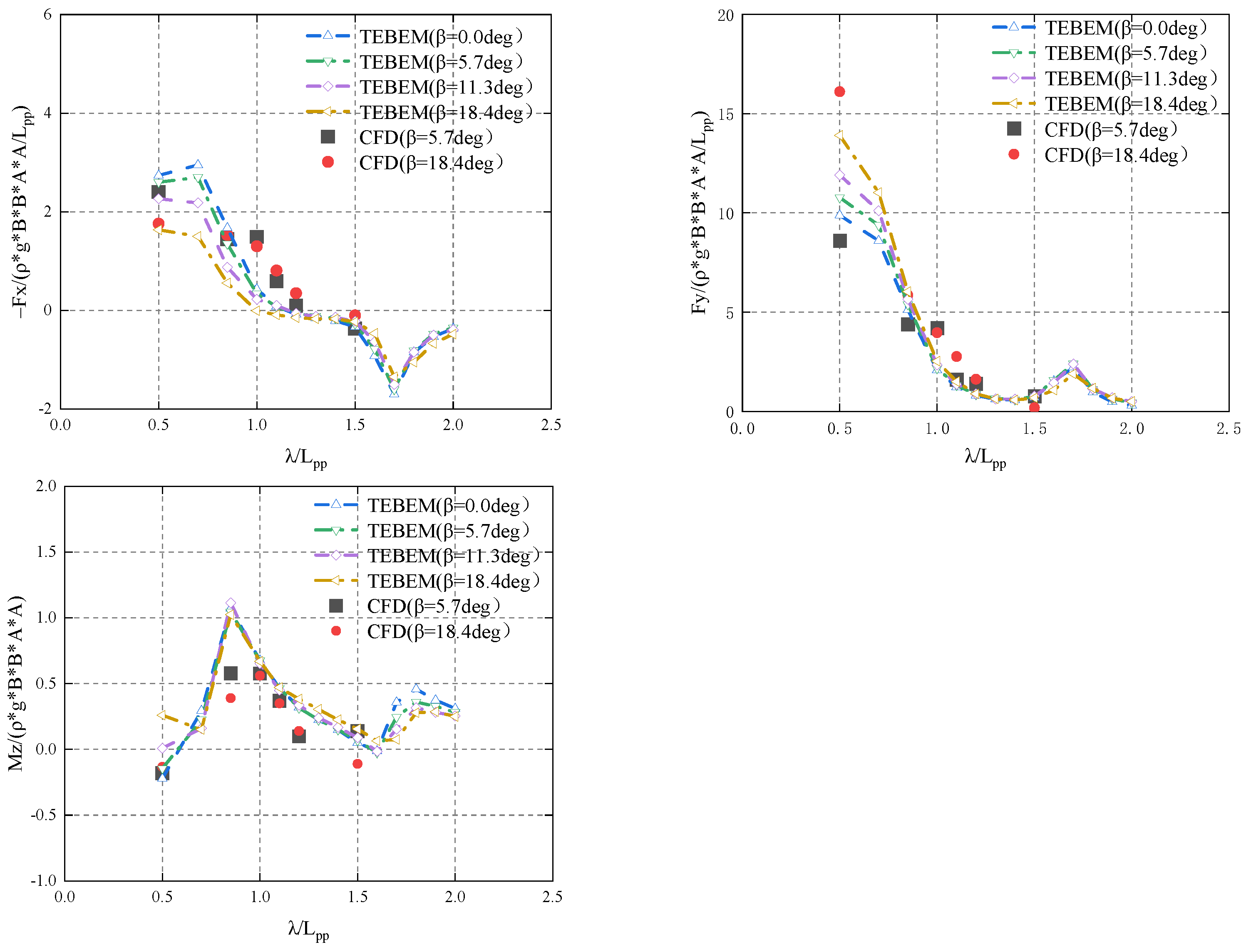
5.3. Wave Drift Loads Analysis of Ships with Different Drift Angles in Oblique Waves

Presently, the wave drift loads are mainly studied with zero drift angle. However, the existence of a drift angle will have a certain influence on the wave drift loads in the turning motion of the ship. Therefore, it is critical to study the wave drift loads of the ship with a drift angle in oblique waves. As described in this section, the RAO of 6-DOF motion and wave drift loads of the KVLCC2 ship are first calculated via TEBEM with H = 0.02 L_PP, χ = 120°, β = 0°, 5.7°, 11.3°, 18.4°, and U = 6.0 kn. Then, the RAO of 6-DOF motion and wave drift loads of the KVLCC2 ship are calculated via the CFD method with H = 0.02 L_PP, χ = 120°, β = 5.7°, 18.4°, and U = 6.0 kn, as shown in Figure 16 and Figure 17. The comparison between the TEBEM and CFD methods shows that the 6-DOF motion, surge, and sway wave drift forces of the ship with β = 5.7° and 18.4° are in good agreement, whereas the yaw drift moments have large discrepancies in the short waves. This is because significant viscous effects due to flow separation occurred in the bow and stern areas, resulting in a small yaw moment calculated by the CFD method. Compared with the CFD results, the accuracy of the wave drift loads of the ship calculated based on TEBEM can meet the requirements.

Figure 16 also shows that the existence of drift angle has little influence on the 6-DOF motion of the ship while having a noticeable effect on the ship’s roll and yaw resonance regions; furthermore, the amplitude near the resonance point of roll and yaw decreases with the increase of drift angle. Figure 17 shows that the drift angle influences the calculation of wave drift loads. Especially when λ/L_PP < 1.0, the surge and sway drift forces have considerable changes. The surge drift force decreases, while the sway drift force increases with the increase in the drift angle. This is because the disturbance of the flow field around the ship is more evident in the short-wave region. Figure 17 also illustrates that the existence of drift angle has little influence on the yaw moment.

The wave drift forces and moment of the ship with drift angle at different wave incident angles are also calculated. Figure 18a–c depict the surge, sway, and yaw wave drift forces and moment of the KVLCC2 with H = 0.02 L_PP, χ = 0°, 30°, 60°, 90°, 120°, 150°, 180°, β = 18.4°, and U = 6.0 kn, respectively. The surge wave drift force increases with the increase in wave direction angle in bow waves in Figure 18a for λ/L_PP ≤ 1.0. The sway wave drift forces reach their maximum at χ = 90°, while the sway wave drift forces are the minimum in the head and following waves. Figure 18c shows that the yaw wave drift moment is negative in stern waves while positive in bow waves.

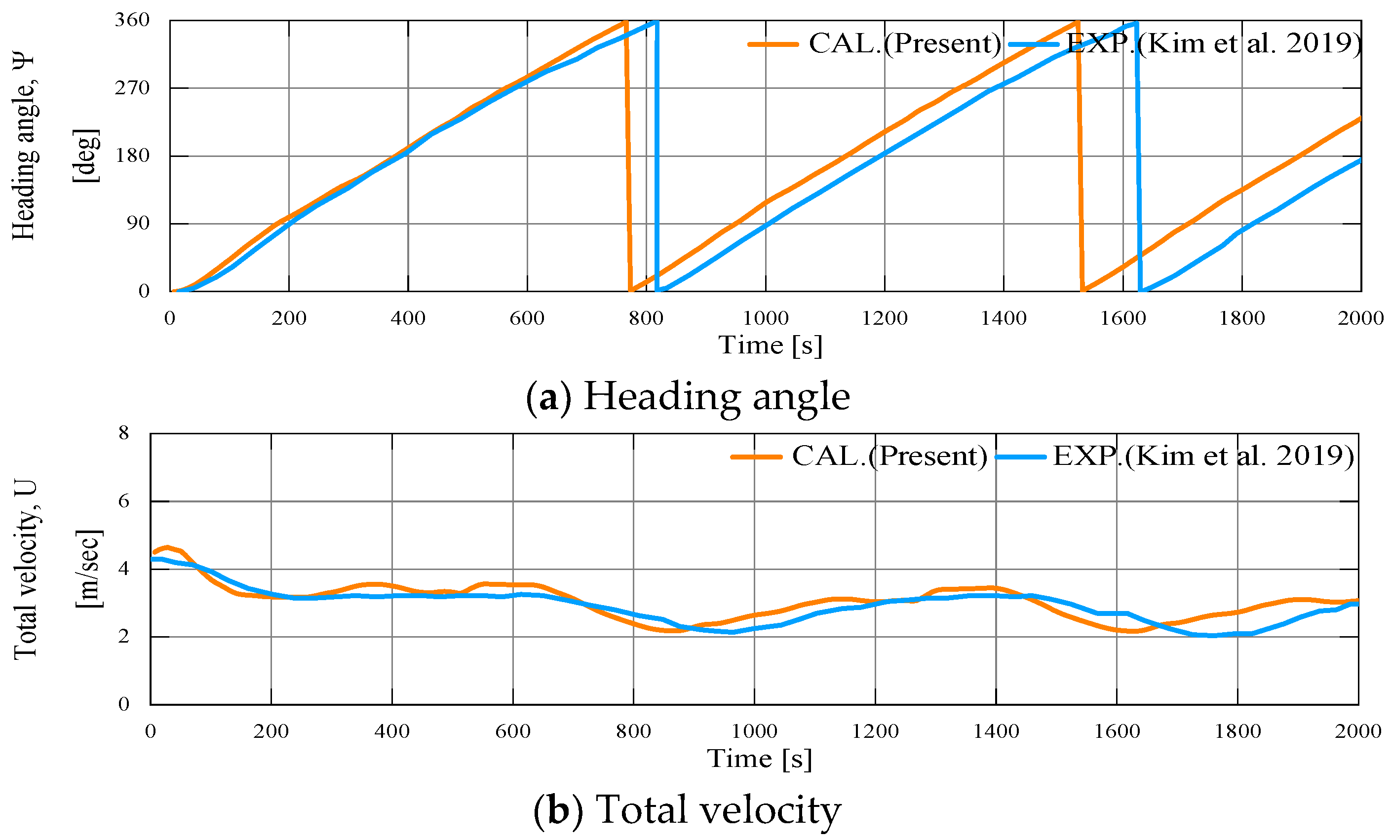
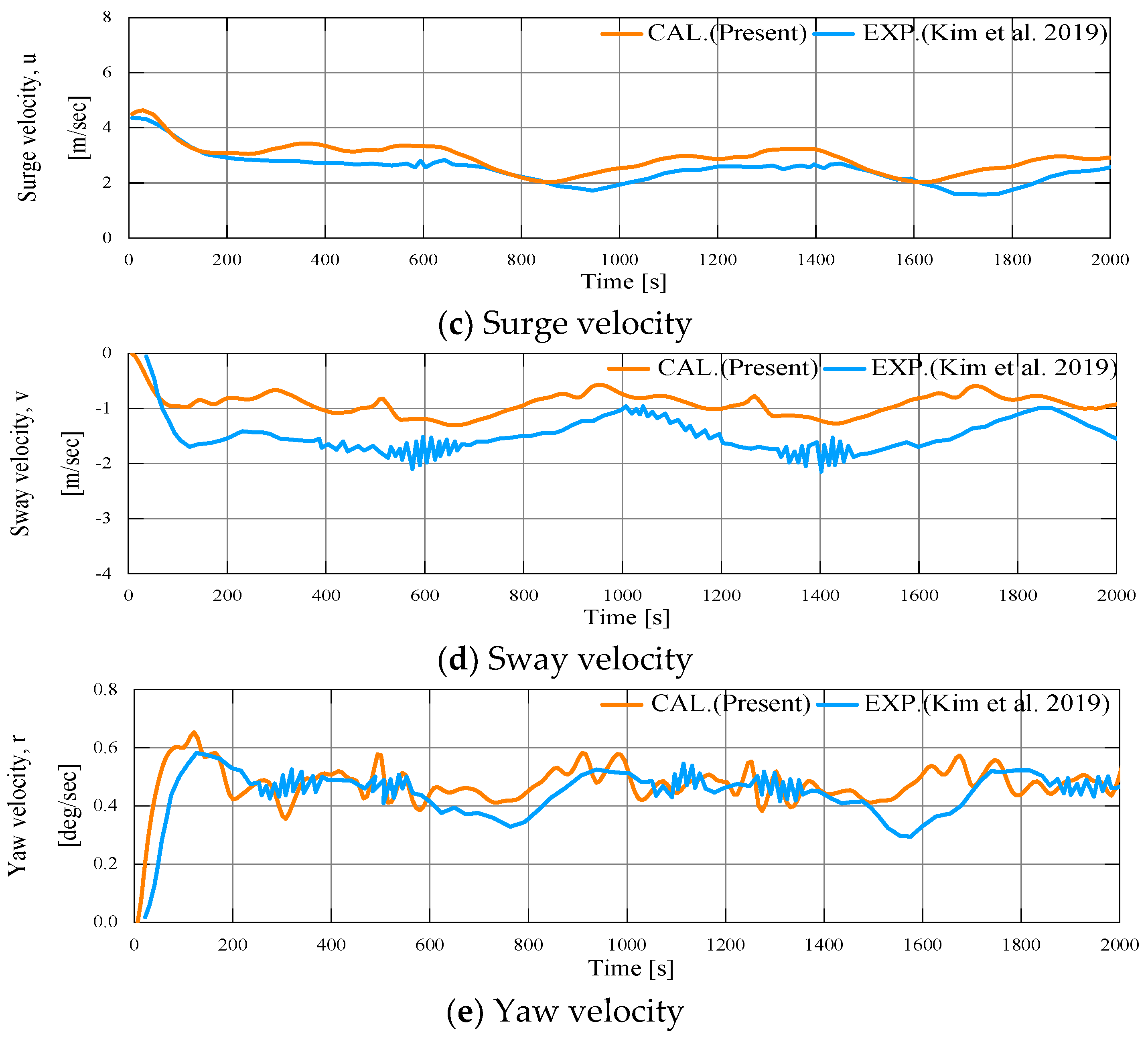
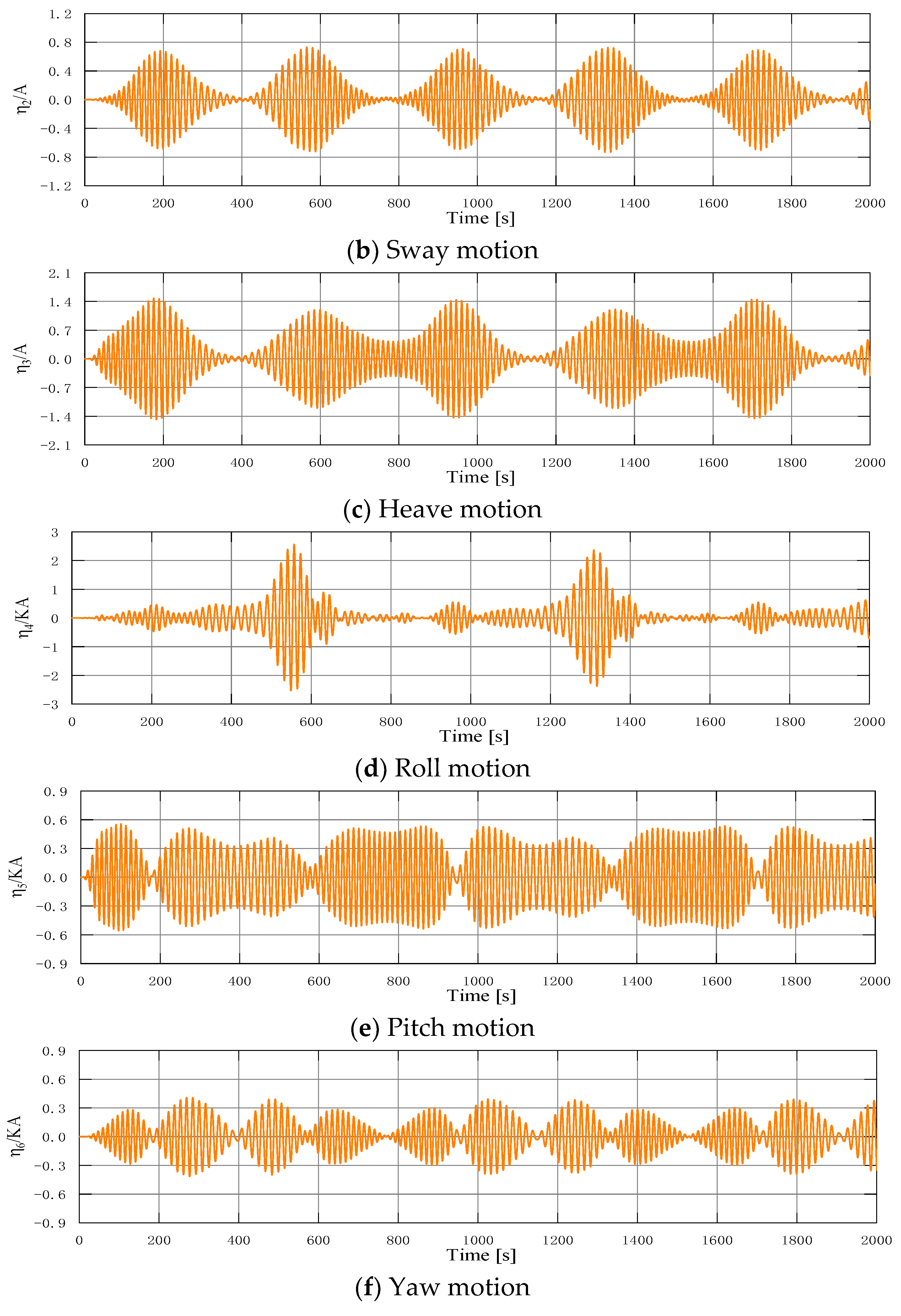
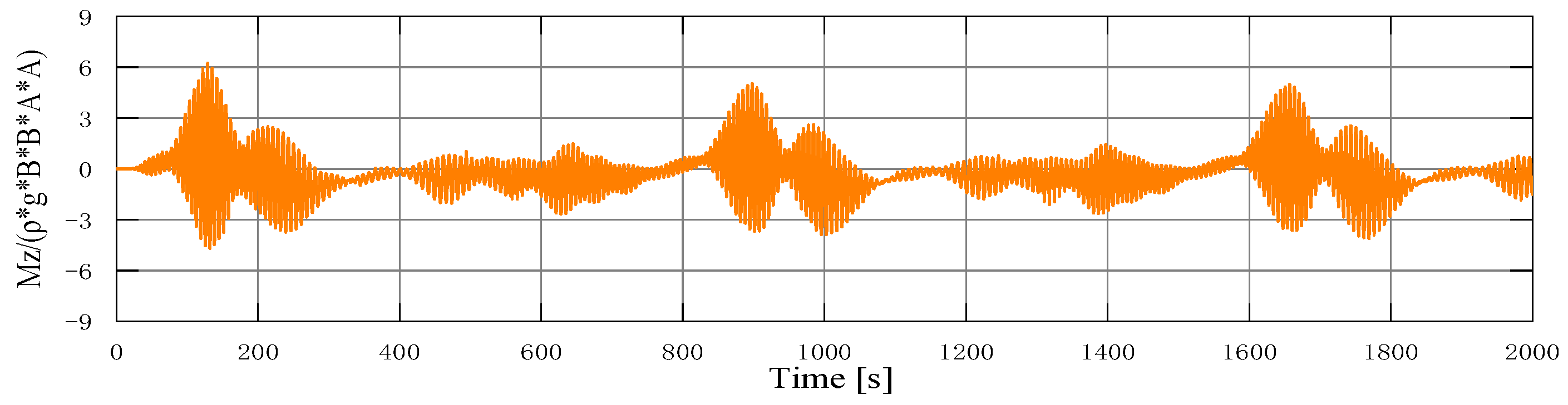
5.4. Time History of Turning Motion in Regular Waves

After the wave drift loads of the ship are solved, the ship’s turning motion in regular waves is calculated. The model ship speed is 1.179 m/s, corresponding to the full ship scale of 15.5 knots in calm water. The propeller speed of the model ship is fixed at 11.8 RPS in all runs. The rudder rate of the model ship is 15.8°/s, which corresponds to the full ship scale of 2.34°/s. The ship’s speed decreases in waves due to the added resistance. The approach speed discussed in this section comes from the experimental value of Kim et al. [8]. The related coefficients and hydrodynamic derivatives used in the numerical simulation are shown in

Table 2. Related coefficients used in the simulation.

Coefficient	Value	Coefficient	Value	Coefficient	Value
${m^{\prime }}_x$	0.022	${R^{\prime }}_0$	0.022	$t_R$	0.387
${m^{\prime }}_y$	0.223	${N^{\prime }}_v$	−0.137	$w_{p0}$	0.388
${J^{\prime }}_z$	0.011	${N^{\prime }}_r$	−0.049	${\alpha }_H$	0.312
${X^{\prime }}_{vv}$	−0.040	${N^{\prime }}_{vvv}$	−0.030	${x^{\prime }}_H$	−0.464
${X^{\prime }}_{vr}$	0.002	${N^{\prime }}_{vvr}$	−0.294	${l^{\prime }}_R$	−0.710
${X^{\prime }}_{rr}$	0.011	${N^{\prime }}_{vrr}$	0.055	$\epsilon$	1.09
${X^{\prime }}_{vvvv}$	0.771	${N^{\prime }}_{rrr}$	−0.013	$\kappa$	0.50
${Y^{\prime }}_v$	−0.315	$t_P$	0.220	$f_{\alpha }$	2.747
${Y^{\prime }}_r$	0.083	$C_1$	2.0	$k_0$	0.2931
${Y^{\prime }}_{vvv}$	−1.607	$C_2$$({\beta }_P$ > 0)	1.6	$k_1$	−0.2753
${Y^{\prime }}_{vvr}$	0.379	$C_2$$({\beta }_P$ < 0)	1.1	$k_2$	−0.1385
${Y^{\prime }}_{vrr}$	−0.391	${\gamma }_R$$({\beta }_R$ > 0)	0.640
${Y^{\prime }}_{rrr}$	0.008	${\gamma }_R$$({\beta }_R$ < 0)	0.395

and derived from Yasukawa et al. [27].

This section describes the simulation of the turning trajectory of the KVLCC2 model with δ = ±35° in calm water and its comparison with the experimental values of Kim et al. [8], as shown in Figure 19. The simulated trajectories generally agree with the experimental results, although the tactical diameter is slightly larger than the experimental value.

Subsequently, the turning motion of the KVLCC2 ship is simulated with wave height H = 0.02 L_pp, wavelength λ = 1.0 L_pp, wave heading χ = 180°, and rudder angle δ = +35°. Corresponding to the full-scale, the numerical simulation time is 2000 s. Figure 20 shows the time history of the heading angle, total, surge, sway, and yaw velocity compared with the experimental values of Kim et al. [8]. As shown in Figure 20a, the variation trend of the heading angle is consistent with the experimental value, but the turning period is slightly smaller than the experimental value. The surge, sway, yaw, and total velocity are periodical changes, as shown in Figure 20b–e. It can be found that the total velocity of the ship is almost consistent with the experimental values and the variation trend of the surge, sway, and yaw velocity are also consistent with the experimental values. The total velocity decreases obviously at 800–900 s and 1600–1700 s, indicating that the speed loss is more significant in bow waves, as shown in Figure 20a. The comparison results show that the numerical model used has sufficient reliability.

Figure 21 shows the time history of the ship’s 6-DOF motion induced by first-order wave forces. It can be seen from Figure 21 that the 6-DOF motion of the ship changes periodically during each turning cycle and can be stably simulated for 2000 s. The roll resonance appears near 557 and 1308 s, and the ship is in beam waves at this time, as shown in Figure 21d. Figure 21b,c show that the sway and heave reach maximum values near the beam waves and minimum values in the heading and following waves. However, the minimum values of yaw motion are reached in the heading, beam, and following waves. Figure 22 shows the time history of the surge, sway, and yaw wave drift forces and moment of the KVLCC2 ship. The surge wave drift force is large near 560 and 1330 s and small near 400 and 1200 s; at that time, the ship is in bow and stern wave conditions, respectively. The sway wave drift force reaches its maximum value at 178, 940, and 1710 s, respectively, and the ship is in the beam waves. The yaw moment is small around 400 s and 800 s, and the ship is in the head and following waves, while it is larger in the bow and stern waves.

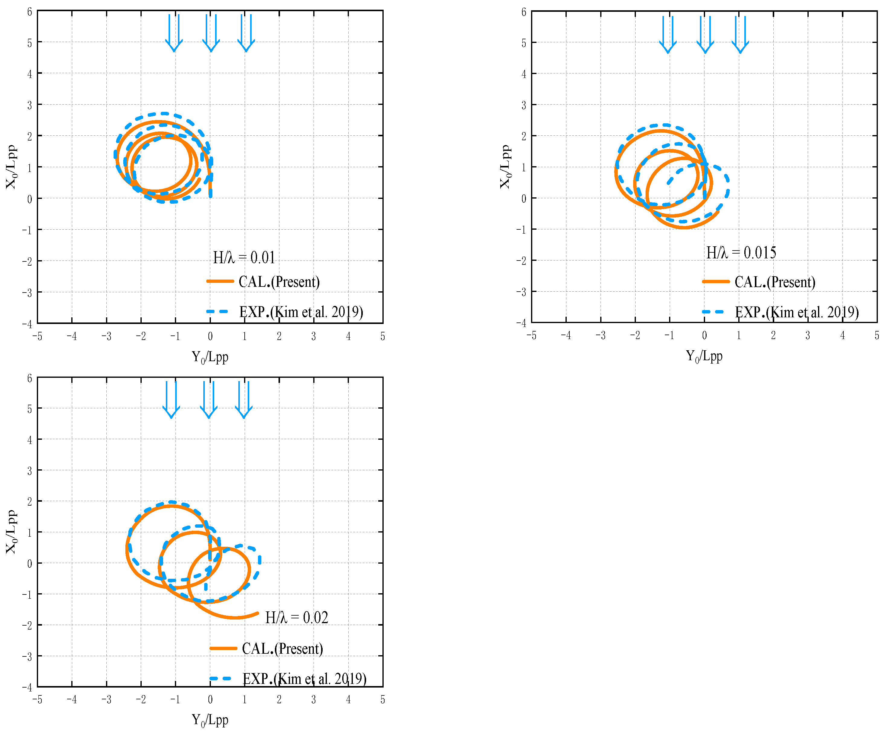
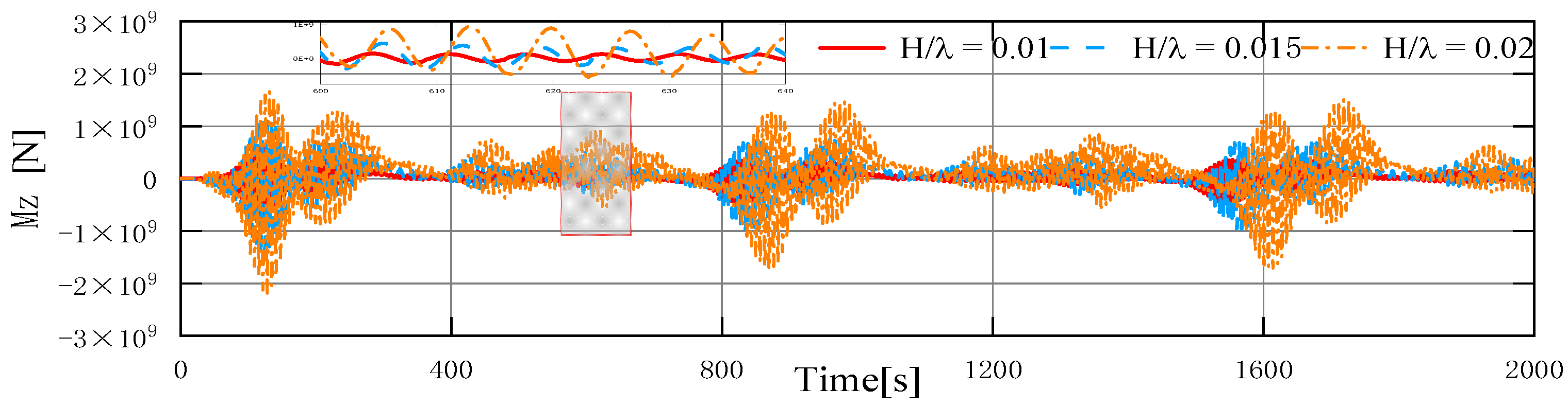
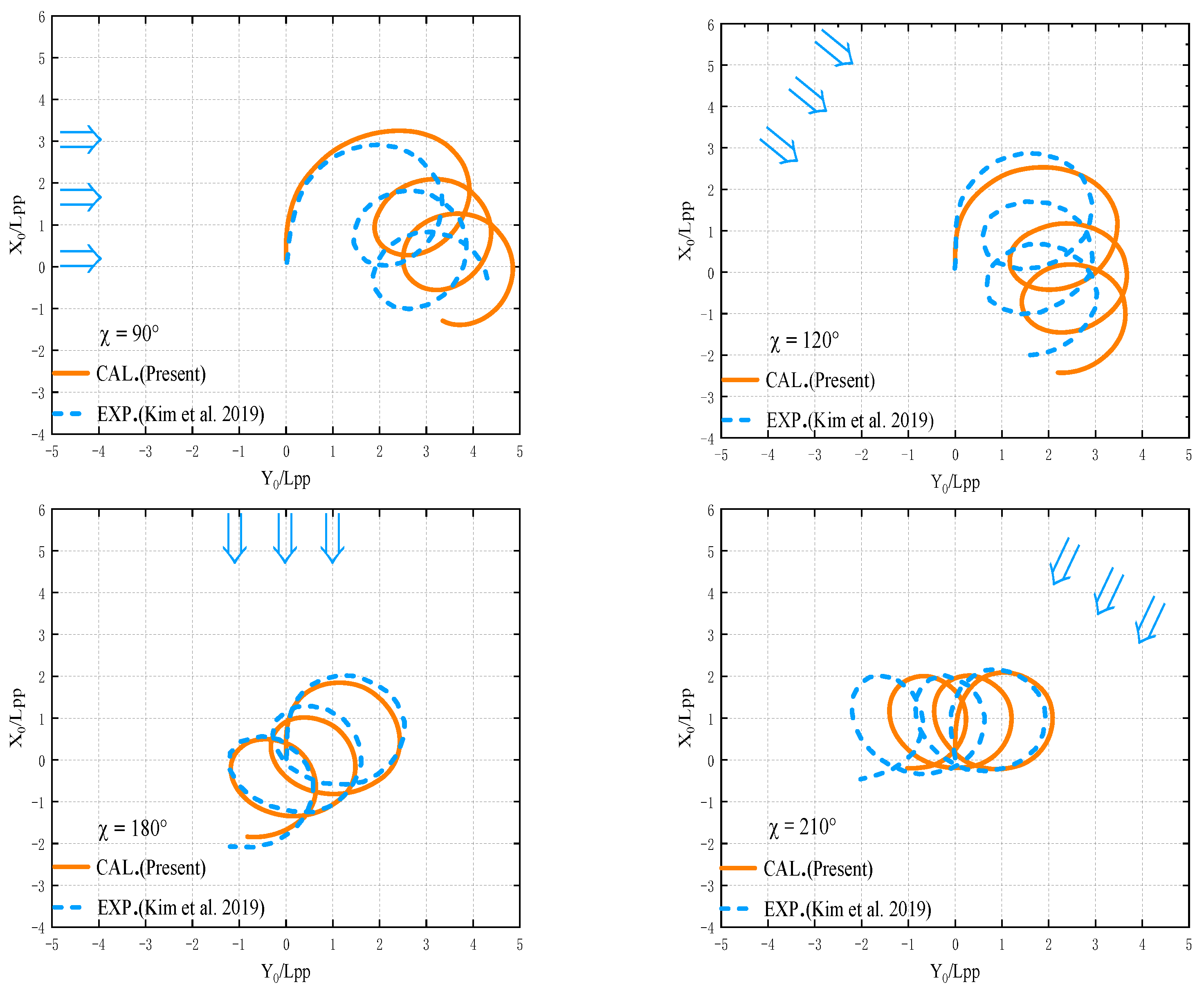
5.5. Simulations of the Turning Trajectory in Regular Waves

The turning motion of the KVLCC2 ship in regular waves with different wavelengths, wave steepness, and wave headings is simulated, which is compared with the experimental values of Kim et al. [8]. The numerical simulation conditions are shown in

Table 3. Numerical simulation conditions.

Rudder Angle, δ (degree)	Wave Heading, χ (degree)	Wave Height, H (LPP)	Wavelength, λ (LPP)	Propeller RPS
+35, −35	No wave (in calm water)			11.8
+35, −35	90, 180	0.02	0.5, 0.7, 1.0, 1.2
+35	120, 210	0.02	1.0
−35	180	0.01, 0.015, 0.02	1.0

.

Figure 23 and Figure 24 compares the turning trajectory of +35° and −35° turns in head waves, respectively, with wave height H = 0.02 L_PP and wavelength λ = 0.5, 0.7, 1.0, and 1.2. As described in this section, 150 wave periods are stably simulated. As shown in Figure 23 and Figure 24, the turning trajectory of the ship drifts along the direction of wave propagation and perpendicular to the wave, and the trend of the turning trajectory is consistent with the experimental value of Kim et al. [8]. Figure 23 shows the trajectory drifting distance is the longest at λ/L_PP = 0.5, and the drifting direction is almost parallel to the wave propagation direction. This is because the surge and sway wave drift forces increase rapidly with the decrease in wavelength. When λ/L_PP = 1.0, the relation angle between the trajectory drift direction and the wave propagation direction is the largest. When λ/L_PP = 1.2, the drift distance is not significant because of the small wave drift loads. Figure 24 shows the drifting distances of −35° turns are close to the +35° turns. However, when the wavelength is 0.5 L_PP, the numerical drifting distances have a slight discrepancy in +35° and −35° turns.

Figure 25 and Figure 26 show similar comparisons of the turning trajectory of +35° and −35° turns in beam waves, respectively. Figure 25 shows a noticeable discrepancy between the numerical simulation and experimental results when λ/L_PP = 0.5. The main reason is that the model of the rudders and propellers in calm water are used in waves, ignoring the unsteady effect of waves on rudders and propellers. Especially in the short wavelength region where the wave period is short; the unsteady effect of rudder and propeller is more obvious. When λ/L_PP = 0.7, 1.0, and 1.2, the trajectory drifting direction and the trajectory drifting distance of the ship are close to the experimental values. Figure 26 shows that the agreement between the numerical results and the experimental results is best when λ/L_PP = 1.0. In summary, the drift tendency of turning trajectories can be obtained via numerical simulation, but some discrepancies remain in the predicted drift distance. According to the comparison results, when λ/L_PP = 0.7, 1.0, and 1.2, the ship’s turning trajectory predicted by the two-time scale model based on TEBEM in waves is acceptable.

Figure 27 shows the turning trajectories of −35° turns in head waves with wavelength λ = 1.0 L_PP and wave height H = 0.01, 0.015, and 0.02 L_PP. Figure 28 shows the time history of the surge, sway, and yaw wave drift forces and moment of the KVLCC2 under −35° turns with a variation of the wave steepness in the head waves. The wave drift loads become larger with the increase in wave steepness, resulting in a significant increase in the drifting distances of the turning trajectory. Figure 27 also shows that the relative drifting angle between the trajectory drift and wave propagation directions also increases slightly.

Figure 29 shows the turning trajectories of +35° turns with wavelength λ = 1.0 L_PP, wave height H = 0.02 L_PP, and wave headings χ = 90°, 120°, 180°, and 210°. As shown in Figure 29, the turning trajectories of the ship are obviously different with the change of wave headings, and the trajectory drifting direction of the ship is in good agreement with the experimental values, but there are discrepancies between the trajectory drifting distances and the experimental values.

Table 4. The advances and the tactical diameters of ships at different wave headings.

Wave Headings [°]	Advances (AD/LPP)	Tactical Diameters (DT/LPP)
90	3.2	3.8
120	2.6	3.5
180	1.8	2.4
210	2.2	2.0

shows the advances and the tactical diameters of ships at different wave headings. It can be seen from Table 4 that the ship’s advances and the tactical diameters differ as the direction of wave propagation changes.

5.6. Analysis of Trajectory Drifting Angle and Distances

The trajectory drifting angle and distances defined by Kim et al. [8] are used to analyze the data of the ship’s turning trajectory, and the data are compared with the experimental values of Kim et al. [8]. The trajectory drifting distance Ddr_090–450 is defined as the vector magnitude between two points corresponding to the heading angles of 90° and 450°, and the trajectory drifting angle Adr_090–450 is the angle between the initial approach direction of the ship and that vector. Other definitions of trajectory drifting angles and distances are similar, where the subscript represents the heading angles at the start and end positions.

Table 5. Comparisons of trajectory drifting angle in head waves [unit: degrees].

δ [°]	χ [°]	H/LPP	λ /LPP	Method	Adr090–450	Adr180–540	Adr270–630	Adr360–720
+35	180	0.02	0.5	Exp.	172	175	173	171
				Cal.	185	171	171	170
				Error	7.56%	−2.29%	−1.16%	−0.59%
			0.7	Exp.	154	147	148	143
				Cal.	144	124	121	121
				Error	−6.49%	−15.65%	−18.24%	−15.38%
			1.0	Exp.	135	125	128	129
				Cal.	141	124	121	122
				Error	4.44%	−0.8%	−5.47%	−5.43%
			1.2	Exp.	160	146	143	163
				Cal.	152	106	99	108
				Error	5.0%	−27.40%	−30.77%	33.74%

and

Table 6. Comparisons of trajectory drifting distances in head waves [unit: L_pp (ship length)].

δ [°]	χ [°]	H/LPP	λ /LPP	Method	Ddr090–450	Ddr180–540	Ddr270–630	Ddr360–720
+35	180	0.02	0.5	Exp.	2.09	2.55	2.24	2.28
				Cal.	2.30	2.07	2.04	2.01
				Error	10.05%	−18.82%	−8.93%	−11.84%
			0.7	Exp.	2.03	2.26	2.16	2.46
				Cal.	2.10	2.27	2.15	2.04
				Error	3.45%	0.44%	−0.46%	17.07%
			1.0	Exp.	0.97	1.11	1.10	1.16
				Cal.	1.06	1.15	1.04	1.01
				Error	9.28%	3.60%	−5.45%	−12.93%
			1.2	Exp.	0.36	0.41	0.35	0.47
				Cal.	0.49	0.59	0.55	0.44
				Error	36.11%	43.90%	57.14%	−0.67%

compare the trajectory drifting angle and distances in head waves. When λ/L_PP = 0.5 and 0.7, the discrepancies in trajectory drifting angle and distance between the numerical results and the experimental results are small, while the numerical discrepancies increase gradually in the long-wave region.

Table 7. Comparisons of trajectory drifting angle in beam waves [unit: degrees].

δ [°]	χ [°]	H/LPP	λ /LPP	Method	Adr090–450	Adr180–540	Adr270–630	Adr360–720
−35	90	0.02	0.5	Exp.	272	273	-	-
				Cal.	256	260	-	-
				Error	−5.88%	−4.76%	-	-
			0.7	Exp.	309	307	309	307
				Cal.	301	306	312	311
				Error	−2.59%	−0.33%	0.97%	1.30%
			1.0	Exp.	332	323	328	329
				Cal.	302	308	297	297
				Error	−9.04%	−4.64%	−9.45%	9.73%
			1.2	Exp.	55	286	296	317
				Cal.	274	297	289	285
				Error	-	3.85%	−2.36%	−10.09%

and

Table 8. Comparisons of trajectory drifting distances in beam waves [unit: L_pp (ship length)].

δ [°]	χ [°]	H/LPP	λ /LPP	Method	Ddr090–450	Ddr180–540	Ddr270–630	Ddr360–720
−35	90	0.02	0.5	Exp.	2.29	2.61	-	-
				Cal.	2.63	2.89	-	-
				Error	14.85%	10.73%	-	-
			0.7	Exp.	1.92	2.10	2.15	2.19
				Cal.	1.63	1.93	2.0	2.03
				Error	−15.10%	−8.10%	−6.98%	−7.31%
			1.0	Exp.	0.66	0.86	0.91	0.88
				Cal.	0.91	1.04	0.96	0.93
				Error	37.88%	10.93%	5.50%	5.68%
			1.2	Exp.	0.12	0.18	0.32	0.38
				Cal.	0.31	0.47	0.52	0.50
				Error	-	-	62.5%	31.56%

compare the trajectory drifting angles and distances in beam waves. The drifting trajectory and drifting angle discrepancies in beam waves are similar to those in head waves. This is probably because of the large error of the numerical results of wave drift loads in the long-wave region compared with the experimental values. Furthermore, the load model of the propeller and rudder is based on the force model under calm water without considering the non-uniformity and unsteady characteristics of the flow field on the propeller surface caused by waves and the 6-DOF motion of the ship, and the influence of the unsteady flow field on the propeller load. Therefore, the propeller rudder load model in waves will be considered in the future. Table 5, Table 6, Table 7 and Table 8 show that as the heading angle of ships increases, the error of the trajectory drifting angle and distance also increases. The reason is that the numerical discrepancies gradually accumulate and increase as the numerical simulation time increases. Although the discrepancies in trajectory drifting angles and distances are large at the long wavelength, the accuracy of numerical simulation is still acceptable compared with the experimental values.

6. Conclusions

This study applies the two-time scale model based on TEBEM to solve the ship’s turning motion in regular waves. The total ship motion is broken down into high-frequency wave-induced motion and low-frequency maneuvering motion. The TEBEM solves the high-frequency seakeeping problem, and the MMG model calculates the low-frequency maneuvering motion. Finally, the wave drift loads are included in the low-frequency maneuvering motion. The major conclusions can be summarized as follows:

1.

The drift angle has a certain effect on the wave drift loads of the ship. In particular, when λ/L_PP ≤ 1.0, the surge drift force gradually decreases while the sway drift force gradually increases with the increase of the drift angle.

2.

Although there are some discrepancies between the numerical and experimental results, the numerical simulation results are still acceptable for the turning trajectory of the KVLCC2 model. The simulated turning trajectories of the ship show that the incident wave significantly influences the ship’s turning motion, and the drifting distance increases with the increase in wave steepness. When λ/L_PP = 1.0, the relation angle between trajectory drifts and wave propagation directions is the largest. The numerical results also show that the turning trajectories of the ship change significantly with the change in wave heading.

3.

The two-time scale model based on TEBEM can effectively solve the turning trajectories of ships in regular waves using maneuvering coefficients and hydrodynamic derivatives in calm water.

In the future, we will further investigate the unsteady flow field distribution and load on the propeller surface to improve the accuracy of the ship’s turning trajectory in waves.

References

1. Yasukawa, H. Simulation of ship maneuvering in waves (1st report: Turning motion). J. Jpn. Soc. Nav. Archit. Ocean Eng. 2006, 4, 127–136. [Google Scholar] [CrossRef] [Green Version]
2. Yasukawa, H. Simulation of ship maneuvering in waves (2nd report: Zig-zag and stopping maneuvers). J. Jpn. Soc. Nav. Archit. Ocean Eng. 2008, 7, 163–170. [Google Scholar] [CrossRef] [Green Version]
3. Yasukawa, H.; Nakayama, Y. 6-DOF simulations of a turning ship in regular waves. In Proceedings of the International Con-ference on Marine Simulation and Ship Maneuverability, Panama City, Panama, 17–20 August 2009. [Google Scholar]
4. Yasukawa, H.; Hirata, N.; Yonemasu, L.; Terada, D.; Matsuda, A. Maneuvering simulation of a KVLCC2 tanker in irregular waves. In Proceedings of the International Conference on Marine Simulation and Ship Maneuverability, Newcastle upon Tyne, UK, 8–11 September 2015. [Google Scholar]
5. Xu, Y.; Bao, W.; Kinoshita, T.; Itakura, H. A PMM experimental research on ship maneuverability in waves. In Proceedings of the 26th International Conference on Offshore Mechanics and Artic Engineering, San Diego, CA, USA, 10–15 June 2007. [Google Scholar]
6. Kinoshita, T.; Bao, W.; Yoshida, M.; Nihei, Y.; Xu, Y.; Itakura, H. Effects of wave drift forces on maneuvering of ship. In Proceedings of the 27th International Conference on Offshore Mechanics and Artic Engineering, Estoril, Portugal, 15–20 June 2008. [Google Scholar]
7. Lee, S.K.; Hwang, S.H.; Yun, S.W.; Rhee, K.P.; Seong, W.J. An experimental study of a ship maneuverability in regular waves. In Proceedings of the International Conference on Marine Simulation and Ship Maneuverability (MARSIM), Panama City, Panama, 17–20 August 2009. [Google Scholar]
8. Kim, D.J.; Yun, K.; Park, J.Y.; Yeo, D.J.; Kim, Y.G. Experimental investigation on turning characteristics of KVLCC2 tanker in regular waves. Ocean Eng. 2019, 175, 197–206. [Google Scholar] [CrossRef]
9. Kim, H.; Akinoto, H.; Islam, H. Estimation of the hydrodynamic derivatives by RANS simulation of planar motion mechanism test. Ocean Eng. 2015, 108, 129–139. [Google Scholar] [CrossRef]
10. Shang, H.D.; Zhan, C.S.; Liu, Z.Y. Numerical simulation of ship maneuvers through self-propulsion. J. Marine Sci. Eng. 2021, 9, 1017. [Google Scholar] [CrossRef]
11. Ma, C.Q.; Hino, T.; Ma, N. Numerical investigation of the influence of wave parameters on maneuvering hydrodynamic derivatives in regular head waves. Ocean Eng. 2022, 244, 110394. [Google Scholar] [CrossRef]
12. Hamamoto, M.; Kim, Y.-S. A new coordinate system and the equations describing maneuvering motion of a ship in waves. J. Soc. Nav. Archit. Japan 1993, 173, 209–220. [Google Scholar] [CrossRef]
13. Sutulo, S.; Soares, C.G. A unified nonlinear mathematical model for simulating ship maneuvering and seakeeping in regular waves. In Proceedings of the International Conference on Marine Simulation and Ship Maneuverability, Terschelling, The Netherlands, 25–30 June 2006. [Google Scholar]
14. Fang, M.C.; Luo, J.H.; Lee, M.L. A nonlinear mathematical model for ship turning circle simulation in waves. J. Ship Res. 2005, 49, 69–79. [Google Scholar] [CrossRef]
15. Lin, W.; Zhang, S.; Weems, K.; Liut, D. Numerical simulations of ship maneuvering in waves. In Proceedings of the 26th Symposium on Naval Hydrodynamics, Rome, Italy, 17–22 September 2006. [Google Scholar]
16. Subramanian, R.; Beck, R.F. A time-domain strip theory approach to maneuvering in a seaway. Ocean Eng. 2015, 104, 107–118. [Google Scholar] [CrossRef] [Green Version]
17. Suzuki, R.; Ueno, M.; Tsukada, Y. Numerical simulation of 6-degrees-of-freedom motions for a manoeuvring ship in regular waves. Appl. Ocean Res. 2021, 113, 102732. [Google Scholar] [CrossRef]
18. Seo, M.G.; Kim, Y.H. Numerical analysis on ship maneuvering coupled with ship motion in waves. Ocean Eng. 2011, 38, 1934–1945. [Google Scholar] [CrossRef]
19. Zhang, W.; Zou, Z.J. A numerical study on prediction of ship maneuvering in waves. In Proceedings of the 30th International Workshop on Water Waves and Floating Bodies, Bristol, UK, 12–15 April 2015. [Google Scholar]
20. Xie, Z.T.; Jeffery, F.; Wang, H. A framework of numerically evaluating a maneuvering vessel in waves. J. Marine Sci. Eng. 2020, 8, 392. [Google Scholar] [CrossRef]
21. Yao, J.X.; Liu, Z.Y.; Su, Y.; Cheng, X.D.; Song, X.M.; Zhan, C.S. A time-averaged method for ship maneuvering prediction in waves. J. Ship Res. 2020, 64, 203–225. [Google Scholar] [CrossRef]
22. Mei, T.L.; Liu, Y.; Ruiz, M.T.; Lataire, E.; Vantorre, M.; Chen, C.Y.; Zou, Z.J. A hybrid method for predicting ship maneuverability in regular waves. J. Offshore Mech. Artic Eng. Trans. ASME 2021, 143, 021203. [Google Scholar] [CrossRef]
23. Jeon, M.; Mai, T.L.; Yoon, H.K.; Kim, D.J. Estimation of wave-induced steady force using system identification, model tests, and numerical approach. Ocean Eng. 2021, 233, 109207. [Google Scholar] [CrossRef]
24. Yasukawa, H.; Hirata, N.; Matsumoto, A.; Kuroiwa, R.; Mizokami, S. Evaluations of wave-induced steady forces and turning motion of a full hull ship in waves. Ocean Eng. 2019, 24, 1–15. [Google Scholar] [CrossRef]
25. Zhang, W.; el Moctar, O.; Schellin, T.E. Numerical study on wave-induced motions and steady wave drift forces for ships in oblique waves. Ocean Eng. 2020, 196, 106206. [Google Scholar] [CrossRef]
26. Duan, W.Y.; Chen, J.K.; Zhao, B.B. Second order Taylor expansion boundary element method for the second order wave radiation problem. Appl. Ocean Res. 2015, 52, 12–26. [Google Scholar] [CrossRef]
27. Yasukawa, H.; Yoshimura, Y. Introduction of MMG standard method for ship maneuvering predictions. J. Mar. Sci. Technol. 2015, 20, 37–52. [Google Scholar] [CrossRef] [Green Version]
28. Chen, J.K.; Duan, W.Y.; Ma, S.; Liao, K.P. Time-domain TEBEM method for mean drift force and moment of ships with forward speed under the oblique seas. J. Marine Sci. Tech. 2021, 26, 1001–1013. [Google Scholar] [CrossRef]
29. Seo, M.G.; Ha, Y.J.; Nam, B.W.; Kim, Y. Experimental and Numerical Analysis of Wave Drift Force on KVLCC2 Moving in Oblique Waves. J. Marine Sci. Eng. 2021, 9, 136. [Google Scholar] [CrossRef]
Figure 1. Two-time scale model of ship maneuvering and seakeeping coupling.
Jmse 10 00993 g001
Figure 2. Space fixed coordinate system and ship moving coordinate system.
Jmse 10 00993 g002
Figure 3. Local coordinate system on the discrete panel.
Jmse 10 00993 g003
Figure 4. Grid diagram of the KVLCC2 ship surface.
Jmse 10 00993 g004
Figure 5. Grid diagram of the free surface.
Jmse 10 00993 g005
Figure 6. Schematic diagram of the horizontal soft spring.
Jmse 10 00993 g006
Figure 7. Time history diagram of the surge wave drift force of the KVLCC2 ship under different panel numbers of the full-body surface.
Jmse 10 00993 g007
Figure 8. Time history diagram of the sway wave drift force of the KVLCC2 ship under different panel numbers of the free surface.
Jmse 10 00993 g008
Figure 9. Time history diagram of the yaw wave drift moment of the KVLCC2 ship under different time-step scales.
Jmse 10 00993 g009
Figure 10. Grid diagram of the longitudinal section of the computing domain.
Jmse 10 00993 g010
Figure 11. Grid diagram of the damping zone of the computing domain.
Jmse 10 00993 g011
Figure 12. Least squares fitting of the surge, sway, and yaw forces and moment of KVLCC2 ship under H = 0.02 LPP, λ = 1.1 LPP, χ = 120°, β = 0°, and U = 6.0 kn.
Jmse 10 00993 g012
Figure 13. The convergence analysis surge, sway, and yaw forces and moment of the KVLCC2 ship under different mesh numbers, time-step scales, and damping zone length, respectively.
Jmse 10 00993 g013
Figure 14. RAO of 6-DOF motion of KVLCC2 under H = 0.02 LPP, χ = 120°, β = 0°, and U = 6.0 kn.
Jmse 10 00993 g014
Figure 15. The surge, sway, and yaw wave drift forces and moment of KVLCC2 under H = 0.02 LPP, χ = 120°, β = 0°, and U = 6.0 kn.
Jmse 10 00993 g015aJmse 10 00993 g015b
Figure 16. RAO of 6-DOF motion of KVLCC2 with H = 0.02 LPP, χ = 120°, β = 0°, 5.7°, 11.3°, 18.4°, and U = 6.0 kn.
Jmse 10 00993 g016aJmse 10 00993 g016b
Figure 17. The surge, sway, and yaw wave drift forces and moment of KVLCC2 with H = 0.02 LPP, χ = 120°, β = 0°, 5.7°, 11.3°, 8.4°, and U = 6.0 kn.
Jmse 10 00993 g017
Figure 18. The surge, sway, and yaw wave drift forces and moment of KVLCC2 with H = 0.02 LPP, χ = 0°, 30°, 60°, 90°,120°,150°, 180°, β = 18.4°, and U = 6.0 kn.
Jmse 10 00993 g018
Figure 19. Comparison of the turning trajectory of the KVLCC2 model with δ = ±35° in calm water. The experimental values were reproduced from [8], with permission from Elsevier, 2022.
Jmse 10 00993 g019
Figure 20. Comparisons of heading angle, surge, sway, yaw, and total velocity of the KVLCC2 under +35° turns. The experimental values were reproduced from [8], with permission from Elsevier, 2022.
Jmse 10 00993 g020aJmse 10 00993 g020b
Figure 21. Surge, sway, heave, roll, pitch, and yaw motions of the KVLCC2 under +35° turns.
Jmse 10 00993 g021aJmse 10 00993 g021b
Figure 22. Surge, sway, and yaw wave drift forces and moment of the KVLCC2 under +35° turns.
Jmse 10 00993 g022aJmse 10 00993 g022b
Figure 23. Comparisons of the turning trajectory of +35° turns with the wavelength variation in the head waves. The experimental values were reproduced from [8], with permission from Elsevier, 2022.
Jmse 10 00993 g023aJmse 10 00993 g023b
Figure 24. Comparisons of the turning trajectory of −35° turns with the wavelength variation in the head waves. The experimental values were reproduced from [8], with permission from Elsevier, 2022.
Jmse 10 00993 g024
Figure 25. Comparisons of the turning trajectory of +35° turns with the wavelength variation in the beam waves. The experimental values were reproduced from [8], with permission from Elsevier, 2022.
Jmse 10 00993 g025
Figure 26. Comparisons of the turning trajectory of −35° turns with the wavelength variation in the beam waves. The experimental values were reproduced from [8], with permission from Elsevier, 2022.
Jmse 10 00993 g026
Figure 27. Comparisons of the turning trajectory of −35° turns with the variation of wave steepness in the head waves. The experimental values were reproduced from [8], with permission from Elsevier, 2022.
Jmse 10 00993 g027
Figure 28. The time history of the surge, sway, and yaw wave drift forces and moment of the KVLCC2 under −35° turns with a variation of the wave steepness in the head waves.
Jmse 10 00993 g028aJmse 10 00993 g028b
Figure 29. Comparisons of the turning trajectory of +35° turns with the variation of wave heading. The experimental values were reproduced from [8], with permission from Elsevier, 2022.
Jmse 10 00993 g029