A Test Method for Obstacle-Avoidance Performance of Unmanned Surface Vehicles Based on Mobile-Buoy–Shore Multisource-Sensing-Data Fusion

Abstract

In order to avoid the influence of the test system itself on the autonomous navigation and performance test accuracy of unmanned surface vehicles (USVs), a test method for the obstacle-avoidance performance of USVs based on mobile-buoy–shore multisource-sensing-data fusion is proposed. In this method, a mobile-buoy-integrated test system is designed (that is, the test instrument is installed on the mobile buoy). The buoy is both the carrier of the test instrument and the obstacle. The software and hardware functions of the test system are realized in modules, and the obstacle-avoidance monitoring function of the USV is realized by the trajectory-tracking method of buoy perception preprocessing and shore adaptive weighted fusion. Then, on the basis of the mobile-buoy–shore sensing-data-fusion method, performance tests and a quantitative evaluation of the obstacle perception, static-obstacle avoidance, and dynamic-obstacle avoidance of the USV were carried out. The results show that: (1) the tested USV can accurately identify the distance between buoys; (2) the three static-obstacle-avoidance performance scores of the single obstacle, continuous obstacle, and inflection-point obstacle are 74.81, 77.14, and 47.61, respectively, and the quantitative evaluation score of the static-obstacle-avoidance comprehensive performance is 66.4; (3) the obstacle-avoidance-performance scores of overtaking, encounter, and cross encounter are about 53.92, 36.51, and 6.48, respectively, and the quantitative evaluation score of the comprehensive performance of the dynamic-obstacle avoidance is 72.36. The above quantitative evaluation results show that the system can: participate in track intervention and obstacle-avoidance monitoring as an obstacle; give the static- and dynamic-obstacle-avoidance quantitative evaluation results in a predetermined way, which verifies the feasibility and effectiveness of the obstacle-avoidance-performance test system of the USV on the basis of mobile-buoy–shore multisource-sensing fusion; and be used for the testing and evaluation of the obstacle-avoidance performance of USVs.

1. Introduction

An important symbol of unmanned-surface-vehicle autonomous navigation is autonomous navigation, and autonomous navigation has a basic requirement, which is obstacle avoidance. Obstacle avoidance refers to the unmanned surface vehicle according to the state information of the collected obstacles in the process of autonomous navigation through the sensor to perceive the static obstacles and dynamic obstacles that hinder its passage, in accordance with a certain method, to effectively avoid obstacle navigation, and finally reach the target point [1,2]. The obstacle-avoidance performance of unmanned surface vehicles is one of the most direct and comprehensive performances for assessing the advantages and disadvantages of its autonomous navigation [3]. The development level of the unmanned-surface-vehicle autonomous-navigation-performance test technology is asymmetrical with its application, the evaluation of the unmanned-surface-vehicle navigation control, diameter planning, diameter tracking, autonomous-obstacle avoidance, and other performances, and lacks the corresponding test standards and test methods to detect the reliability of unmanned surface vehicles. The existing ship standards cannot meet the needs of the comprehensive performance test of unmanned surface vehicles [4,5]. Thus, research on the comprehensive performance of USVs is imminent, and it is evaluated through research on the performance of the navigation control, path planning and tracking, berthing, obstacle avoidance, and so on, which are generally considered to be critical behaviors of USVs. Hyo-Gon Kim et al. adapted an algorithm DWA according to the international regulations for preventing collisions at sea, taking into consideration both the distance from and time to the closest point of approach in different marine scenarios, defined in the COLREGs as containing head-on encountering, crossing, and overtaking [6]. Hong X et al. utilized the image-semantic-segmentation model, as well as the faster RCNN model, to enable the USV to understand the environment and then make an obstacle-avoidance action with the appliance of the VFH+ algorithm [7]. Bibuli M et al. propose a nonlinear Lyapunov-based control law for driving the USV to track along a designed path, and they brought the followed target together into the control model with an extra virtual control degree of freedom attached to it [8]. Xiao G et al. conducted a series of CFD simulation cases regarding the wind–wave coupling effect in a ship-berthing-safety assessment [9]. Gongxing Wu et al. established a mathematic manipulating system of a ship berthing in a narrow port that deals with different target parameters in the approach process, turning process, and berthing process [10]. Phanthong T et al. succeeded in real-time path planning and avoiding stationary undersea obstacles for an USV equipped with a multibeam forward-looking sonar and GPS system with the A* algorithm [11].

In terms of the research on the performance test method of USVs, Caccia M. et al. used the prototype catamaran Charlie to conduct sea tests to test the effectiveness of the extended Kalman filter and the simple PID control law on the control tasks, such as the automatic heading, automatic speed, and straight-line driving of USVs [12]. Liu Y. et al. tested the formation-path-planning performance of a USV in environments of single and multiple moving obstacles [13]. Villa J. et al. conducted a simulation and physical test. In the simulation, a predefined path was formed through a series of GPS waypoints, and there was a fixed obstacle in the middle of the path to test whether the USV could avoid obstacles; the physical test was conducted in Pyhajarvi Lake, Tampere, Finland, to test its path-tracking and static-obstacle-avoidance performances, for which the static obstacle was a buoy [14]. Wang H. et al. put forward suggestions for the USV test site. At the technical level, they believe that it is necessary to establish a multi-physical-environment perception model of the real sea area to form a visual, traceable, and reconfigurable USV-test-environment platform [15].

In terms of buoy-function-application research, Tender L. et al. studied a microbial fuel cell (MFC) for a buoy with the function of measuring the air temperature, pressure, relative humidity, and water temperature, and they configured it as a real-time line-of-sight RF telemetry data device. This MFC was used to power the meteorological buoy and enable it to operate for a long time [16]. Rhinefrank K. et al. designed a buoy generator that uses the vertical component of wave motion to generate power. The generator is composed of a permanent-magnetic-field system (installed in the center of the translation axis) and an armature, which generates power (installed on the buoy). The transformer shaft is fixed on the seabed, and the buoy/float moves the armature coil relative to the permanent magnet transformer to induce voltage [17]. Kato T. et al. configured GPS on a buoy to predict the tsunami and accurately locate the tsunami source, and they recorded the tsunami caused by the Kii Peninsula earthquake on 5 September 2004 [18]. McPhaden M. et al. combined the tropical atmospheric ocean/triangular transoceanic buoy network in the Pacific Ocean, the tropical Atlantic prediction and research mooring network, and the non-Asian Australian monsoon analysis and prediction research mooring network in the Indian Ocean to form a global tropical mooring-buoy array to provide real-time data for climate research and prediction [19]. Venkatesan R. et al. designed a low-cost sensor-buoy system for monitoring the shallow-water environment, equipped with a sbe39 sensor, MCP9700 sensor, and young61302l sensor to realize the remote monitoring of the temperature, ocean pressure, and temperature and atmospheric pressure, respectively, and the feasibility was verified by an operation test in the marine environment [20]. Albaladejo C. et al. deployed six mooring buoys with sensors to collect the underground oceanographic parameters in the bay in real time. At the discontinuous depth of the bay, the buoy system monitored the timeseries of the temperature and salinity in the water column 500 m away from the ground, and the vertical profile of the water flow in the water column up to 100 m, to continuously measure the surface meteorological and oceanographic parameters of the timeseries [21]. Fefilatyev S. et al. configured cameras on buoys, proposed a visual ship-detection and tracking algorithm based on buoys on the high seas, and developed a horizon-detection scheme. Verified by large datasets, the ship-detection accuracy reached 88%, and the horizon-detection and positioning accuracy reached 99% [22]. Byun J. et al. proposed an in-situ gamma ray spectral analysis system based on a buoy (shallow-water light), which had a thickness of 7.6 cm × 7.6 cm NaI (Tl). The detector is used for the remote and real-time monitoring of gamma-ray-emitting radionuclides in surface seawater [23]. Kinugasa N. et al. developed a mooring-buoy observation system for the continuous monitoring of seabed crustal deformation by using global navigation satellite system acoustic technology, which can detect seabed displacement at the centimeter level [24].

Tang Y. et al. designed an SZF-type wave-buoy system, with a self-weight of 105 kg and a displacement of 140 kg, which can independently and regularly (or continuously) measure the wave height, cycle, and direction. The buoy system can be divided into the buoy part and shore part. The buoy is powered by a lithium-ion battery, and VHF digital communication is adopted for the buoy–shore communication [25]. Aiming at the problem of the low conversion efficiency between the wave energy and generator, Song B. et al. established a mathematical model of an ocean buoy and deduced the parameters. Through simulation experiments, it was concluded that the performance of the wave generator was related to the wave height and frequency. They then improved the buoy-power-generation system based on the wave energy [26]. To improve the use efficiency of sonar buoys in anti-submarine warfare, Ling Q. et al. proposed a linear-array multistatic sonar-buoy system and circular-array multistatic sonar-buoy system, which expanded the search area and saved the number of buoys compared with the traditional passive buoy array [27]. Kong W. et al. designed a meteorological measurement buoy that is based on the Beidou communication system. The buoy adopts a low-energy-consumption microprocessor and is equipped with a solar-charging module, which has excellent performance in collecting hydrological data [28]. Zhang D. et al. considered the problem of a buoy dynamic tracking ship on the water surface, dynamically modeled the buoy, and proposed an adaptive control algorithm based on a neural fuzzy network so that the buoy can adjust the movement route and position of the buoy to the required target with relatively less position error [29]. Aiming at the problem of the low accuracy of the traditional current-measuring buoy, Lu H. et al. located the position information of a buoy through a GPS module, and transmitted the effective data to the shore host computer through ziggee vehicle terminal communication after the analysis and judgment of the processor [30]. It can be seen from the above research that, at present, buoys are mostly used as marine observation platforms, which are mainly used for hydrometeorological information collection and observation, sea area monitoring, and underwater acoustic positioning. The research results are rich, while the obstacle-avoidance static obstacles of USVs that are based on mobile buoys have a single function.

In the research on obstacle recognition that is based on multisource-data fusion, Lu T. et al. fused the target classification algorithm of the radar-observation model and the ESM-sensor-observation model on the reconnaissance problem in a battlefield-situation assessment based on the Bayesian probability distribution, refused the data recognition of target types by constructing a new combined likelihood function, and improved the probability of the successful classification to 0.95 in a shorter time [31]. Wang P. et al. proposed an improved JPDA multitarget tracking algorithm for the key problem of intelligent transportation with multisensor data association. Combined with the correlation sequential association method, they associated the multisensor data probabilistically, and then fused the multisensor data convexly, which can continue the target tracking if the sensor loses the effective target for a short time [32]. Gan X. et al. found that the AIS recognition system of maritime ships and the traditional radar-information-fusion method have great limitations. Based on the Yolov3 framework, the traditional AIS + radar sensing method is combined with the camera recognition method to fuse the position and visual information, and the correct detection rate of 94.35% was achieved in the Huangpu River Channel of Shanghai [33]. Aiming at the multisensor fusion technology of radar ship positioning, and based on the particle-filter-tracking fusion method, Chen K. applied the improved filter method to the weighted fusion of infrared and radar, which effectively improved the fusion accuracy and tracking effect [34].

In summary, the research progress of unmanned-surface-vehicle performance testing at home and abroad is as follows: (1) unmanned-surface-vehicle test sites have been established and put into use at home and abroad, and the autonomous navigation performance of unmanned surface vehicles has been evaluated by holding events; (2) at present, buoys are mainly used for hydrometeorological information collection and observation, sea area monitoring, and underwater acoustic positioning, and the research results are rich, while the test research on the obstacle-avoidance performance of unmanned surface vehicles that is based on mobile buoys is still in its infancy; and (3) most of the buoys that are currently applied do not have a power system and can only be used as static obstacles in the unmanned-surface-vehicle obstacle-avoidance-performance test, and the function is single.

In order to avoid the influence of the test system itself on the autonomous navigation and performance test accuracy of unmanned surface vehicles (USVs), the main goal of the research presented in the article was to combine the urgent needs of the obstacle-recognition and obstacle-avoidance performance tests of unmanned surface vehicles, and a test method for the obstacle-avoidance performance of USVs that is based on mobile-buoy–shore multisource-sensing-data fusion is proposed.

The novelties presented in the article are the design of a set of obstacle-avoidance-performance test systems for USVs that is based on mobile-buoy–shore sensing-data fusion, the obstacle-avoidance-performance test research that was carried out, and the verification of the feasibility and effectiveness of the test system.

The remainder of the article is arranged as follows: in the second section, we present the design of the obstacle-avoidance-performance test system; in the third section, we present the obstacle-avoidance-performance test and results analysis; in the fourth section, we present the discussion; and in the final section, we present the conclusion.

2. Design of Obstacle-Avoidance-Performance Test System for USVs

During sailing on the sea, the obstacle-avoidance scenes that are encountered by USVs are ever changing. To ensure the consistency of the obstacle-avoidance behavior of USVs in the scenes encountered as much as possible, it is necessary to ensure that the scenes in the test scheme are representative. According to whether the obstacles move during navigation, the obstacle avoidance of USVs is divided into static-obstacle avoidance and dynamic-obstacle avoidance. The design of the obstacle-avoidance test scheme for USVs should be gradual, from shallow to deep. It is necessary to consider not only the actual operating environment of USVs, but also the collision-avoidance rules, conventions, etc. [35,36,37].

2.1. Architecture Design of Obstacle-Avoidance-Performance Test System for USVs

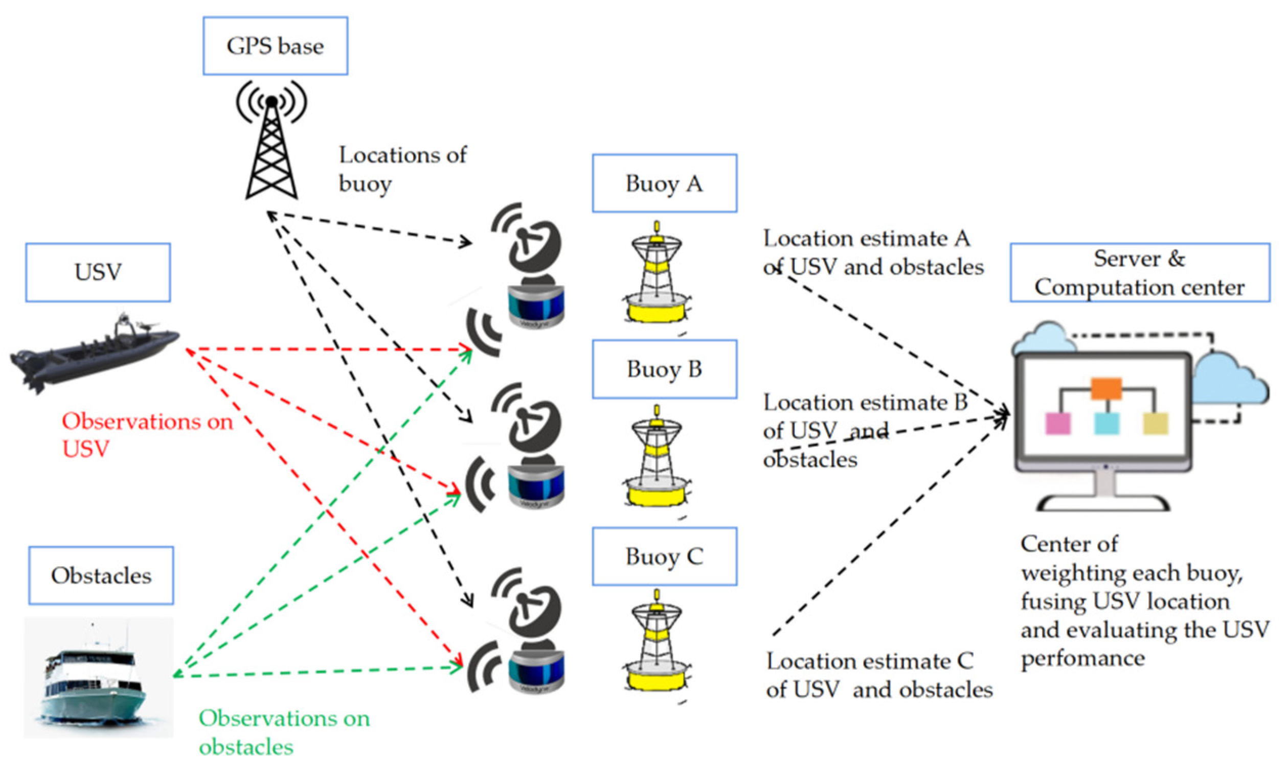
By integrating the advantages and disadvantages of a distributed test system and centralized test system, a hybrid test system of mobile-buoy–shore multisource-sensing-data fusion between the distributed and centralized systems was designed, as shown in Figure 1.

It can be seen from Figure 1 that the local buoy in this test system also needs an independent data processor. The sensing equipment on the local buoy senses the data of all objects in the test sea area, detects and identifies the USV and other static obstacles, filters out the useless data, and then calculates the real-time navigation position data of the USV. The observation information of the buoy, other obstacles, and the USV in the navigation path is transmitted to the shore data-processing center. After receiving the data of each local buoy, the shore data-processing center weights and fuses the obstacle-avoidance navigation data of the USV and calculates the corresponding technical evaluation indicators. Because the sensing data is preprocessed at the buoy and then sent to the shore, the hybrid test system can reduce the communication pressure. The data are integrated and processed in the shore data-processing center, which can make full use of the high-computing-power equipment arranged on the shore to ensure the integrity of the navigation data of the USV. Compared with the distributed system, it can more accurately restore the obstacle-avoidance trajectory of the USV and reduce the error of the navigation data index.

The obstacle-identification information during the navigation of the USV is expressed in the follow-up coordinate system of the USV. To achieve the goal of monitoring the obstacle-avoidance performance of the USV, the buoy monitoring system needs to observe the position change of the USV in the obstacle-avoidance process and the relative position with the obstacle. The buoy system obtains the same information from a completely objective angle and forms the evaluation of the obstacle-avoidance performance of the USV under reliable conditions.

2.2. Method of Multisource-Sensing-Data Fusion Based on Mobile-Buoy–Shore

The mobile buoy equipped with the sensor can accurately extract the sensing amount of the concerned target within the viewing-angle range of the sensor, and can obtain its orientation, category, and other information through further calculation to provide key environmental information input and information preprocessing for the whole test system. In this process, the lidar data are filtered and segmented to significantly reduce the search range, and the region-weighted improved OBB point-cloud-matching algorithm is used to accurately detect and locate the three-dimensional target point-cloud cluster. Each mobile-buoy monitoring point can provide observation data from different directions to the shore base. According to the local signal reflection intensity of each sensor, the shore base adopts a niche genetic algorithm to adaptively evaluate the weight and integrate various parameters to reduce the influence of noise and wave interference in the process of the local system detection and calculation and improve the robustness of the monitoring system.

2.2.1. Method of Multisource-Sensing-Data Fusion Based on Mobile Buoy

Different sensors follow different information-acquisition frequencies. To ensure the accuracy of an observation, it is obvious that the observation action and measurement of the position of the machine need to occur at the same time, or at least at a similar time. Time information and time matching are needed in the simultaneous interpretation of different sensors. The local mobile-buoy sensing system realizes information exchange through the ROS multirobot architecture. The DGPS, lidar, and camera in the test system publish the data through the topic under the ROS framework, and the host-computer main program subscribes to the topic between the same local network. As a channel, the topic ensures that the information flow can only be transmitted between the publisher and the receiver through the topic. Recognition and positioning mainly rely on a DGPS receiver and 3D lidar. The data released by them have their own transmission protocols. Before data fusion, it is necessary to interpret their data-message format in detail.

Through DGPS to obtain the centimeter-level positioning of the buoy itself, and through the three-dimensional lidar to obtain the USVs, other buoys, sea surface, land, and other ship point-cloud three-dimensional positions (the radar point-cloud-data filter, the discrete point cloud, sea surface point cloud, etc.), filter, and then filter the radar point-cloud-cluster segmentation and the formation of several clusters of point clouds, and finally calculate the geometric characteristics of each cluster of radar point clouds, match them with the geometric characteristics of unmanned boats, screen out the point-cloud clusters that represent unmanned boats, and solve the real-time positioning of the unmanned boats after fusion.

The DGPS mobile receiving terminal receives the GPS correction value sent by the server at shore, and then corrects the GPS positioning data of its own terminal, by which it obtains accurate positioning data. The data output usually follows the NMEA (National Marine Electronics Association) protocol. Lidar usually obtains the correction of the timestamp with the engagement of the pulse-per-second message (i.e., PPS clock), which is also provided by the GPS message. PPS clock data is organized as HHMMSS.sss, which is in UTC standard. To synchronize the DGPS mobile receiving terminal with the 3D lidar, we set the final data transmitted by the DGPS terminal in GPGGA format, which is Global Positioning System fix data, and one of the message protocols of the GPS organizing time message identical to HHMMSS.sss. The real-time longitude and latitude, and the corresponding time in UTC standard of the buoy, will then be analyzed in the ROS main program according to the GPGGA protocol.

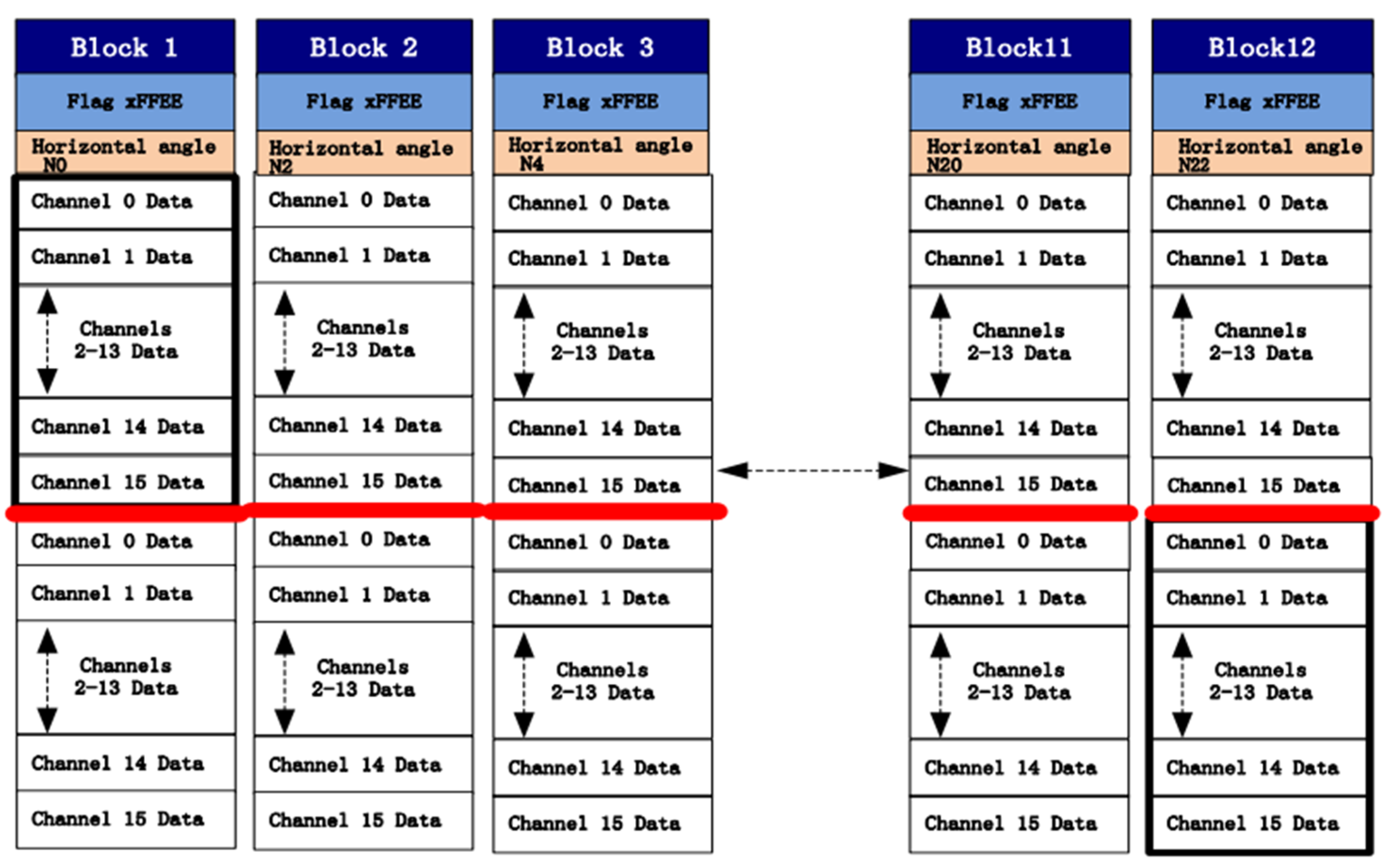
We also need to specify the data from 3D lidar, which includes measurement data, such as the distance value, angle value, reflection-intensity value, and timestamp. In single-echo mode, point-cloud data contain 12 data blocks, and each data block contains two groups of 16-channel point-cloud data, measured in the packaging order. The data-message structure is shown in Figure 2.

As can be seen from Figure 2, 16 channels correspond to the number of lines of the radar; that is, each channel corresponds to a vertical-angle value. Each data block only carries the horizontal azimuth of the laser emitted by the first group of channels (0). Since the radar rotates and emits light at a uniform speed, and the emission time and interval time of adjacent channels are unified, the corresponding values of the horizontal angles of the remaining 31 channels in the block can be obtained by interpolation according to the initial horizontal azimuth of the adjacent data blocks. The data size in a single channel is 3 bytes. The high 2 bytes represent the distance, and the low 1 byte represents the reflection intensity. In addition, in terms of timing, the radar generates an additional 4-byte timestamp (accurate to 3.125) at the end of the last channel in the packet μs). According to the luminous interval and luminous time of each channel, the timestamp of the point-cloud data received by 32 channels can be calculated retrospectively. We programmed the main program to obtain the information in format of GPGGA, and to extract the UTC timestamp when the point cloud is detected (the highest accuracy is 10 ms). We then managed to register the accurate time when one buoy positions itself, as well as the time when the feature clouds of the ROI are extracted by the correspondingly assembled 3D lidar. After all, the logical premise of reasonably fusing sensing data requires us to guarantee the simultaneity of the localization and observation.

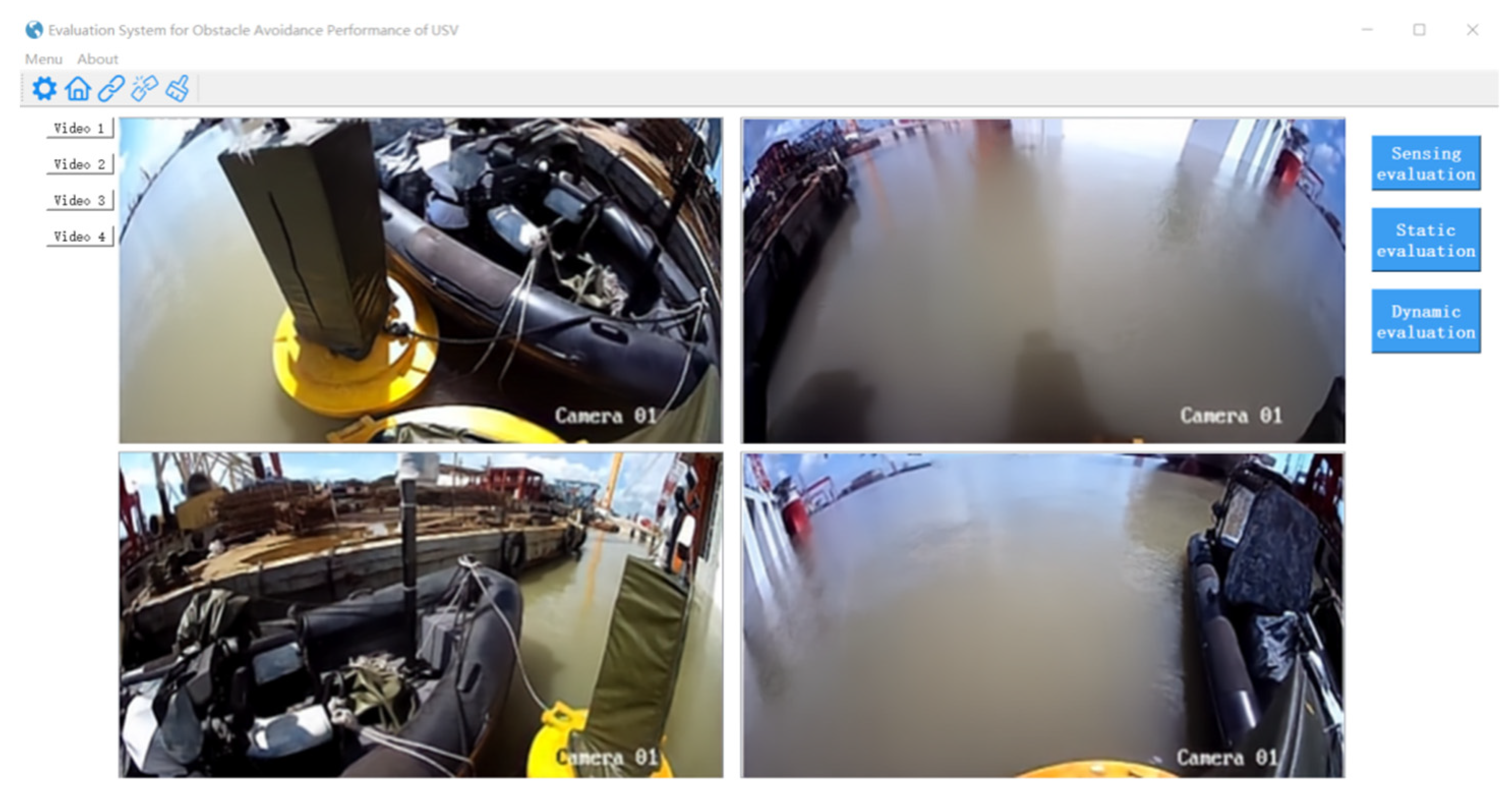
The camera sensor does not need to carry out other data processing. It only needs to release the camera topic, access the information flow of the ROS main program, and send it to the shore through wireless-image-transmission radio for the video monitoring of the test process. The left- and right-angle cameras, and their monitoring interface, are shown in Figure 3.

As can be seen from Figure 3, message filters are used in the ROS multisensor system. The filters receive different types of messages from multiple nodes and output the messages synchronously only when each source has the same timestamp, obtains the $gpzda field in DGPS as the standard time signal, and waits for the lidar data matched with the timestamp according to the UTC time frequency. The time proximity value is set to 0.2 ms, which is allowed. This is equivalent to filtering out redundant lidar data with a clock margin of 10 ms, which can still maintain a high detection accuracy for the detection and recognition system.

2.2.2. Adaptive Weighted Fusion Algorithm Based on Niche Genetic Algorithm at Shore

Each local buoy system obtains its own DGPS information and environmental perception information. After preliminary processing, the information fed back to the shore base includes the coordinates of the OBB center point of the USV point cloud, the coordinates of the OBB center point of the obstacle, and the timeseries information. The independent observation process of each local buoy system will be affected by the random error disturbance of its own area. To dynamically give the confidence of each local sensor system, after each local buoy system sends the independent observation results to the shore base, the shore base dynamically determines the data weight of each buoy by using a niche genetic algorithm, and the measured values of each buoy are adaptively weighted and fused to obtain the fusion judgment results of the absolute coordinates and relative orientation of the USV and the obstacle.

The positioning accuracy of each local buoy can reach the centimeter level. However, the perception of three-dimensional objects will be affected by random errors. The same three-dimensional calculated by each buoy will have position coincidence errors. Therefore, it is necessary to evaluate the discrete data according to specific parameters, and adaptively allocate the fusion weight to determine the final fusion position.

Suppose that at time (k), a total of N local buoys perceives the three-dimensional body of the same water surface, and the unbiased estimation, together with the error covariance matrix ($P_{k/k}^{Mi}$) of the position vector of a three-dimensional body on a water surface, were then sent to the shore base by the local buoy (M₁, M₂, M₃, M₄, …, M_N) after perceptual computing. Each buoy is given a weight coefficient (W_i ∈ {W₁, W₂, W₃, W₄, …, W_N}), with which the three-dimensional volume position ($\tilde{X}$) in one single observation is obtained based on the local buoy data, as shown in Formula (1).

$$\{\begin{array}{ll}\tilde{X}=& {\displaystyle \sum _{i=1}^N}{W}_i^{*}{X}_{k/k}^{m_i}\\ & {\displaystyle \sum _{i=1}^N}{W}_i^{}\end{array}$$

(1)

So far, we can obtain the most reliable set of constraints when we need to fuse. So far, we still need a set of reliable constraints on the $W_i$ to ensure that, when the constraint is satisfied, the $\tilde{X}$ obtained by fusion is the most reasonable. For this purpose, we calculate the variance matrix of the observed value, as shown in Equation (2). Since the perceptual calculation of any local buoy is completed by the local processor, and the hardware is independent of each other, as shown in Equation (3), it can be considered that the position calculation errors between different buoys under a single observation are also independent of each other, and the calculation of the overall variance matrix is further obtained as shown in Equation (4).

$$P=E[\left(X-\tilde{X}{)}^2\right]$$

(2)

$$E\left[\left(X-X_K^{M_i}\right)*\left(X-X_K^{M_j}\right)\right]=0,i\ne j \in \left(1, \dots , N\right)$$

(3)

$$P=E[{\displaystyle \sum }_{i=1}^N{W}_i^2*\left(X-X_k^{M_i}{)}^2\right]={\displaystyle \sum }_{i=1}^N{W}_i^2*P_i^{M_i}$$

(4)

It can be seen from Equation (4) that the overall variance (P) is jointly determined by each weighted weight. The smaller its value, the more the overall fusion result can conform to each local observation, as shown in Equation (5). According to the extreme value theory of the multivariate quadratic function, the conditions for obtaining the minimum value of the P are as follows, and the corresponding minimum value of the P is shown in Formula (6):

$$W_i^{*}=1/(P_k^{M_i}*{\displaystyle \sum }_{i=1}^N\frac{1}{P_k^{M_i}})i\in \left(1,\dots ,N\right)$$

(5)

$$P_{min}={({\displaystyle \sum }_{i=1}^N\frac{1}{P_k^{M_i}})}^{-1}$$

(6)

It can be found from Equations (5) and (6) that the optimal allocation weight of each buoy changes dynamically with the covariance ($P_{min}$) of the observation matrix at each time. We found the optimization goal of giving the weight ($W_i$) to make it meet the $P_{min}$. However, the traditional direct calculation of the weight ($W_i$) needs to search the local nearest-neighbor-coordinate points to find the solution that satisfies the variance ($P_{min}$). In order to avoid complicated calculation, we further explore other characteristics of the $W_i$.

We hoped to find a calculation parameter other than the coordinate value and give an a priori calculation formula of the $W_i$ (7). Obviously, when the distance between the buoy and the measured three-dimensional body is very close, the sensing data can only detect part of the contour of the three-dimensional body, and the observation data of this angle are not enough to accurately calculate the geometric center coordinates of the three-dimensional body. Therefore, in this case, the sensor weight should reflect the characteristics of low reliability. On the contrary, when the buoy is far away from the measured three-dimensional body, the significant change in the sensing data can indicate that there is a three-dimensional body in this position, which has a high reliability. In this case, the sensor should be given a high weight. Therefore, the prior formula of the buoy weight allocation should be able to express the inverse proportional relationship between the perceived distance and the reliability, and the reflection intensity (Iny) in the sensing data can better meet the change trend in the perceived distance. Therefore, the preset ($g$, $f$) is the confidence threshold of the radar reflection intensity. If it is lower than the lower threshold, the allocation weight will be increased, and if it is higher than the upper threshold, the allocation weight will be reduced. The following piecewise weighted proportion function is constructed:

$$W_i=\{\begin{array}{c}{c}_1-j_1*Iny,Iny>g\\ \mathit{T},\mathit{g}<\mathit{I}\mathit{n}\mathit{y}<f\\ c_2+j_2*Iny,Iny<f\end{array},0\le W_i\le 1$$

(7)

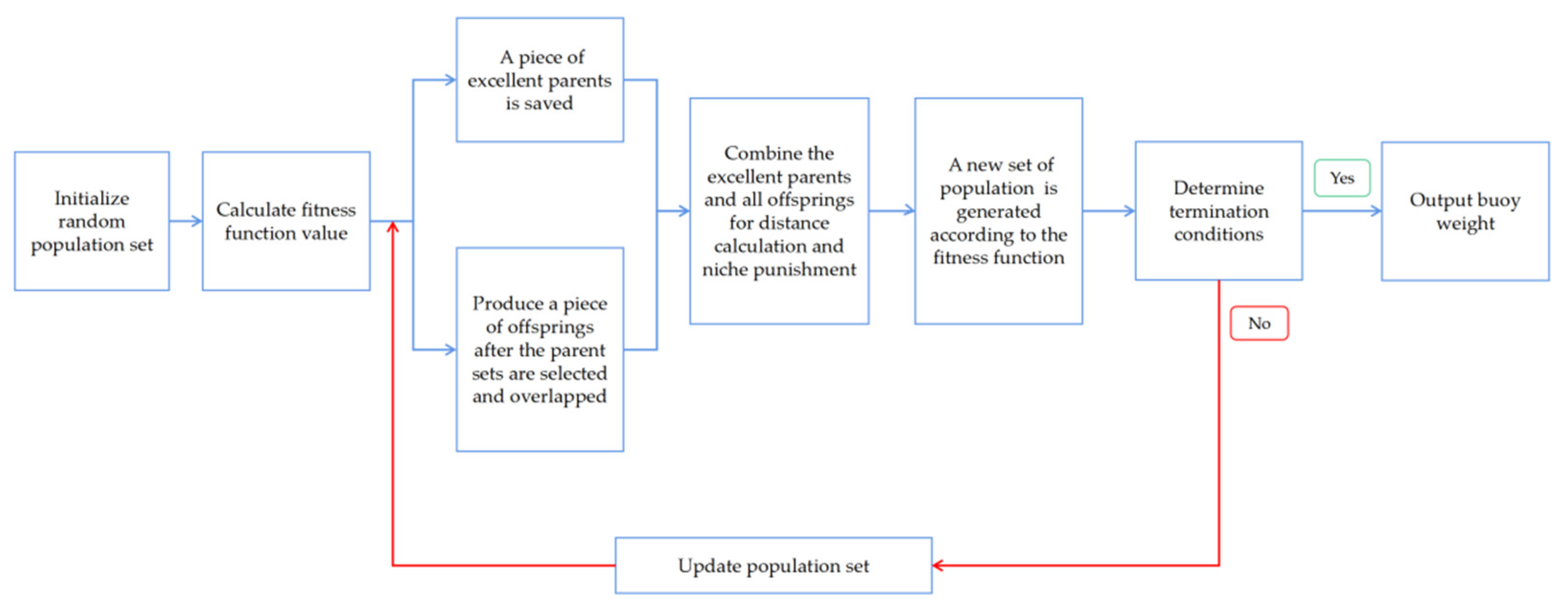
Unknown parameters ($j_1,j_2,c_1,c_2,T$) are introduced into Equation (7). At this time, the niche genetic algorithm combines the diversity of the traditional genetic algorithm and improves the processing of the multipeak-optimization problem. It can search the optimal multivariate unknown variables in the global range so that the error and variance of the fusion results are as small as possible in the known radar-reflection-intensity parameter space. The niche genetic algorithm selects the optimal value in line with the optimization goal through the processes of generating an original population, designing the fitness function, selection, crossover, and mutation. The niche-genetic-algorithm framework for adaptively assigning local buoy weights according to the lidar reflection intensity is shown in Figure 4.

How the algorithm was organized is shown in Figure 4 and is further explicated below for the convenience of comprehension:

a. Generate the original population. According to the prior knowledge of the data reliability and radar reflection intensity, when the reflection intensity is very strong, the measured target is very close to the buoy sensor, the data accuracy is low, and the $W_i$ should be given a value of nearly 0. In the case that $c_i>>j_i$, we may set the initial value as $c_i=1000j_i$. When the reflection intensity is extremely small (that is, close to the measurement limit of the sensor), the data accuracy is also low. Thus, the $W_i$ should also be given a value of nearly 0 (that is to say, $c_2=0$). The genetic algorithm realizes discrimination by coding and calculating the Euclidean distance between different codes, coding the coefficient vector of an a priori formula as $b_i=\left(j_{1i},j_{2i},c_{1i},T\right)$, and then randomly generates an initialization population, ($\left\{b_1,b_2,b_3,b_4,\dots ,b_N\right\}$) with a number of $N$;

b. Design the fitness function. According to the relationship between the coefficient vector and the optimization objective, the fitness function is used to determine whether the genetic algorithm can be retained between generations, and to evaluate whether the parents and newly generated offspring can enter the next generation. The construction of the fitness function should meet the requirements of the optimization objectives. Construct the following fitness function, as shown in Equation (8):

$$Fit\left(r,t\right)=\frac{1}{1+\left(X-X_k^{M_i}\right)+P_{min}}$$

(8)

c. Memory operation. Arrange the coefficient vector set in reverse order according to the FIT value, and remember the first $M$ coefficient vectors;

d. Select the operation. Select the coefficient vector population. The higher the evaluation value of the fitness function in ②, the more likely it is to be selected into the next generation population. The roulette selection operator is used for intergenerational selection, according to Formula (9):

$$p_i=\frac{Fi{t}_i}{{{\displaystyle \sum }}_{i=1}^{N}Fi{t}_i}$$

(9)

e. Cross operation. Select a new generation of groups and perform a single-point-crossover operation for everyone. ⑤ Mutation. A set of different coefficient vectors is used to replace a set of values in the original coefficient vector set to generate a new coefficient vector set, and the mutation operator based on real-value coding is adopted;

f. Niche elimination operation. Compare the Euclidean distance between two coefficient vectors. Compared with the preset distance threshold (L), if the Euclidean distance is less than the threshold, the fitness function in the pair of coefficient vectors is smaller, and the penalty function is applied to further reduce the fitness-function value, making it difficult for them to enter the next generation group in the intergenerational selection to ensure that only one elite solution vector is deduced within the radius (L). The niche elimination operation ensures the diversity of coefficient solutions, reduces the distance between solutions, and can be dispersed in the solution space.

2.3. Calculation of Indicates in Obstacle-Avoidance Missions

With the weight of each buoy that is given by the last section, the ordinates of the locations of the detected 3D objects, the USV and obstacles included, can finally be ascertained. However, the time sequences of the ordinates are given without categorizing them into the USV or obstacle groups. In other words, there may be more than two ordinates received in one single sequence, and we may not directly ascertain the very ordinate of the USV. Unlike the common practice of adopting the deep-sort method to distinguish and track the target that is popular in image recognition, we only need to figure out whether the point is a static point between a few adjacent time sequences by means of matching and calculating the Euclidean distance of the corresponding point. One point will be categorized into the static obstacle while the distance is less than the threshold that was set previously. Considering that the test of the obstacle avoidance of USVs can be conducted in a zone where there is no other ship sailing around, and the locations of mobile buoys can be identified, the remaining point can be identified as the USV with a large degree of credibility.

Moreover, the indicates of obstacle avoidance also need to be defined. In a static scenario, the distance of the reaction dst is defined as the distance between the very point (marked as A) where the USV starts to continuously drift from the original route and the location of the obstacle that intersects it ahead in the route. The distance of the regression dst in a static scenario is defined as the distance between the location (marked as B) where the USV totally reverts to the route and the location of the avoided obstacle. The duration between the two-event moment is defined as the time of avoidance (Tst). Moreover, in a dynamic scenario, the distance of the reaction ($d_{dy}$), as well as the time of avoidance ($T_{dy}$), are similarly defined as dst and Tst. While the minimum distance in the second scenario is more strictly limited, by stating this we are referring to the fact that $d_{dy}^{min}$ is equal to the closest distance during the whole obstacle-avoiding period. The distances above are all calculated as the Euclidean distance between two ordinates in longitude and latitude, which is omitted for brevity. The logic block diagram is shown in Figure 5. Aimed at determining the actual point of the drifting and reverting to further ascertain the indicates we declared above, the program framework mainly caches the probable drifting point or reverting point into a group, the first one of which would not be set as the true result unless the size of a similar point detected continued to accumulate and exceed the threshold. Moreover, the very obstacle that truly influences the route is also evaluated during the framework.

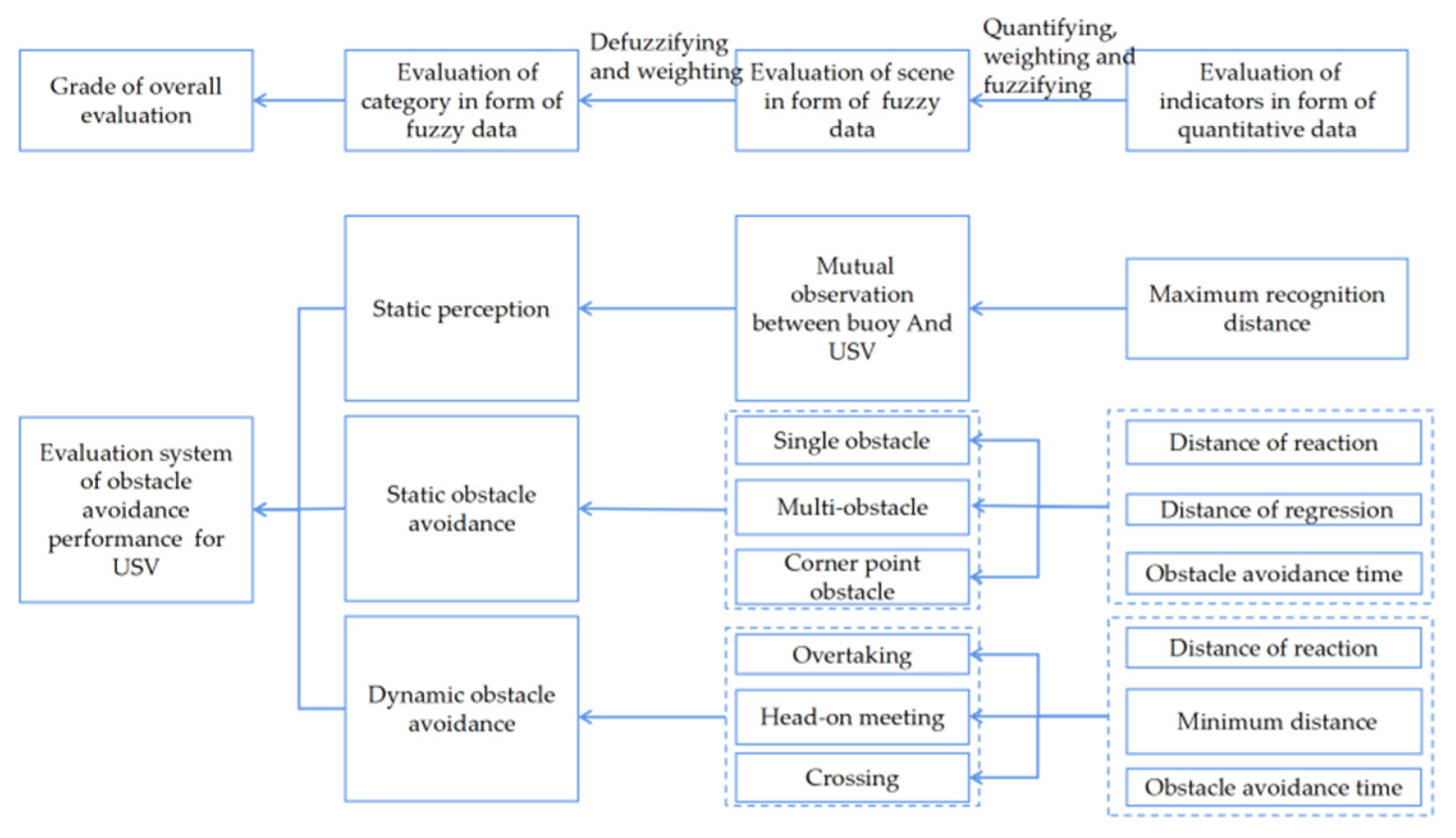
2.4. Quantitative Evaluation Method Based on Cost Function and Fuzzy Comprehensive

The test system for the obstacle-avoidance performance of USVs using fused data between buoys and the server at shore, which is proposed in this paper, is composed of a set of evaluation systems for testing the obstacle-avoidance performance of buoys and USVs, as shown in Figure 5.

As can be seen from Figure 5, the system includes three evaluation categories, and each evaluation category selects several evaluation scenarios. In a single evaluation scenario, specific data indicators need to be given. Each data index is comprehensively calculated by the sensor-data-fusion system, and then the obstacle-avoidance performance is quantified and evaluated according to the data. The performance of a single evaluation scenario can be quantitatively evaluated according to its data indicators, and the evaluation-category level needs to be comprehensively scored according to the performance of all evaluation scenarios. However, the evaluation data participating in the category-level evaluation are not suitable for complete quantitative representation. In the process of the quantified data from the underlying data index→evaluation scene→evaluation category, the comprehensive performance information of the USV obstacle avoidance in the specific scene will be lost in the second stage, and so fuzzy processing needs to be introduced.

Xiao, G. et al. developed an evaluation system that combines cost-function evaluation and fuzzy-comprehensive evaluation [36]. The data-index-evaluation layer comprehensively generates the cost-function value ($c_1,c_2,c_3$) under the current scene by using the measured data of the next layer. On this basis, the fuzzy evaluation matrix ($S$) is given. Combined with the quantitative weight matrix (Q) that conforms to the analytic hierarchy process and the fuzzy-evaluation results of the evaluation-scene level, the evaluation results of this category are calculated at the upper level (evaluation-category level), as shown in Formula (10). Then, the evaluation result is multiplied by the corresponding score of the fuzzy index:$\varphi ={\{1.0,0.8,0.6,0.3\}}^T$. The final score obtained by the calculation is shown in Equation (11):

$$B=Q*S$$

(10)

$$score=100*B*\varphi$$

(11)

2.5. Obstacle-Avoidance-Performance Test Scheme of USV

Taking the USV with a length of 3–20 m and a speed of 15 kn as an example, combined with the actual operation scene and referring to the standards of the literature [1,2], the buoy base has a diameter of 1.5 m, a height of 2.4 m, and a draft of about 20 cm, and it can be regarded as a cylindrical obstacle with a diameter of 1.5 m and a height of 2.2 m. As an obstacle, this specification buoy will not increase the test cost, and it has strong mobility, which improves the test economy and efficiency.

The buoy system is equipped with three-dimensional lidar, an RGB camera, and a DGPS receiver. The laser point-cloud OBB bounding box is used to detect the target. In the static and static-and-dynamic obstacle-avoidance links, the absolute coordinates of the USV and its relative position relationship with the obstacle are calculated and sent to the shore receiving end. The data sequences measured by multiple buoys at the same time are weighted and fused on the shore to mark the obstacle-avoidance trajectory of the USV based on the shore. The dynamic data of the obstacle-avoidance process are evaluated according to the obstacle-avoidance index, and the comprehensive score of the obstacle-avoidance process of the USV is given after the test.

Firstly, the buoy tests the close sight distance between the buoy and the hull, and the relative distance between the USV and other static obstacles on the water surface, under static conditions, and corrects the observation error of the buoy test system. The USV initiates an autonomous navigation through unknown static obstacles in the test sea area, deploys static buoy groups in different areas of the route to monitor the whole process of obstacle-avoidance navigation, and returns to the actual obstacle-avoidance route of the USV. After receiving the buoy data, the shore platform uses the niche genetic algorithm to determine the weight of each piece of buoy data, and it uses the adaptive weighting method to fuse each piece of buoy data to determine the navigation position and obstacle position of the USV. The reaction distance, time, obstacle-avoidance distance, and other key data of the hull in the process of obstacle avoidance are recorded to realize the obstacle-avoidance navigation monitoring of the USV. After the test, the comprehensive evaluation of this obstacle avoidance is given through the developed software platform.

As a part of the obstacles perceived by the USV during navigation, the buoy can trigger the USV to avoid obstacles; at the same time, the environmental-information-acquisition system carried by the buoy makes it a mobile observation point to record the obstacle-avoidance process of the buoy from the perspective of a third party and evaluate its performance. A set of multipoint monitoring systems is formed between each local buoy and the USV. Compared with the evaluation based on the information collected by the position and attitude sensor independently carried, the system has better anti-interference performance, and the mobile buoy integrates obstacles and the observation body, which can more flexibly implement the dynamic-obstacle-avoidance experiment and form a more comprehensive obstacle-avoidance navigation-monitoring system.

3. Obstacle-Avoidance-Performance Test and Results Analysis of USV

To verify the position measurement effect of the USV based on the test system of mobile buoys, the static-position monitoring experiment of unmanned boats was carried out in the offshore waters test field, and the buoy was placed in the test field, where there was a fixed position and a known longitude and latitude of 18.12 m long, 5.24 m wide, and 5.49 m high. The three buoys were placed in positions from 30 to 40 m, from 60 to 70 m, and from 90 to 100 m from the USV, and three sets of experiments were performed. The test data are shown in

Table 1. Comparative data analysis of positioning of unmanned surface vehicle.

Group	Actual Latitude and Longitude of USV/°	Latitude and Longitude of the Shore-Based Fusion Solution/°	Error/m
1	(113.645048, 22.702319)	(113.645059, 22.702327)	1.44
2	(113.645048, 22.702319)	(113.645057, 22.702327)	1.28
3	(113.645048, 22.702319)	(113.645060, 22.702315)	1.31

.

From Table 1, it can be concluded that the position information of the unmanned boat after the shore-based fusion of each piece of the local buoy data of the test system has an actual longitude and latitude error of about 1.34 m with the unmanned boat, which is about 7.4% of the total length of the USV, which has a minimal impact on the performance test results of the USV, can meet the test requirements of the unmanned-boat obstacle-avoidance performance, and verifies the effectiveness of the test system in monitoring the location of the USV.

According to the test scheme in 2.4, a mobile buoy was arranged in a test site with a length of 900 m, a width of 800 m, and a depth of 8 m to carry out the obstacle-perception, static-obstacle-avoidance, and dynamic-obstacle-avoidance performance tests of the USV. The basic measurement data were calculated by using the mobile-buoy test system and the shore data-processing center, and the obstacle-avoidance performance of the tested USV was quantitatively evaluated according to the quantitative evaluation model.

3.1. Obstacle Perception Test

The obstacle-perception-test experiment is as follows: The mutual measurement of the sight distance between local buoys and USVs in the range of 50–75 m. According to the test steps in 2.4, the buoy as an obstacle moves to the bow direction of the USV in the test sea area in advance. The visible volume of the buoy on the water is measured in advance, and the visible size boundary of the buoy on the water in the test sea area is about 1.51 m × 1.51 m × 2.10 m. The accuracy angle of the lidar used in the experiment is 0.09 degrees in the horizontal range, and 2 degrees in the vertical direction. The accuracy of the point-cloud data is affected by the distance. The allowable observation error in the horizontal direction is 1.57 × 10⁻³ m/m, and that in the vertical direction is 3.49 × 10⁻² m/m. Three groups of independent experiments were carried out. The data samples are shown in

Table 2. Mutual measurement results of sight distance between local buoy and USV.

Experimental Group	Planned Distance/m	Buoy Enclosure Size (Measured by USV)/m × m × m	Distance (Measured by USV)/m	Distance (Measured by Buoy)/m	Ranging Accuracy of USV	Is It Qualified?
The first group	50	1.56 × 1.53 × 2.22	51.48	51.23	0.49%	yes
	55	1.53 × 1.53 × 2.21	56.47	56.69	0.39%	yes
	60	1.52 × 1.50 × 2.16	59.98	59.91	0.12%	yes
	65	1.50 × 1.48 × 2.16	65.13	65.26	0.20%	yes
	70	1.49 × 1.45 × 2.13	70.36	70.52	0.23%	yes
	75	1.46 × 1.43 × 2.10	75.47	75.69	0.29%	yes
	80	1.44 × 1.40 × 2.05	80.51	80.24	0.34%	yes
	85	1.37 × 1.35 × 2.01	85.00	85.23	0.27%	yes
	90	1.29 × 1.24 × 1.92	92.19	92.48	0.31%	yes
	95	1.18 × 1.09 × 1.73	97.23	95.33	1.99%	no
The second group	50	1.53 × 1.50 × 2.18	52.79	58.01	9.00%	no
	55	1.49 × 1.44 × 2.15	55.06	55.03	0.05%	yes
	60	1.42 × 1.40 × 2.09	60.59	60.37	0.36%	yes
	65	1.34 × 1.33 × 2.06	65.77	66.01	0.36%	yes
	70	1.30 × 1.27 × 1.96	70.23	70.06	0.24%	yes
	75	1.26 × 1.19 × 1.81	76.53	75.02	2.01%	no
The third group	50	1.49 × 1.49 × 2.13	49.65	49.98	0.66%	yes
	55	1.45 × 1.44 × 2.09	55.01	55.23	0.40%	yes
	60	1.41 × 1.39 × 2.07	62.36	62.13	0.37%	yes
	65	1.38 × 1.35 × 2.07	66.78	66.90	0.18%	yes
	70	1.33 × 1.32 × 2.01	70.23	70.01	0.31%	yes
	75	1.24 × 1.29 × 1.95	78.23	75.32	3.86%	no

.

It can be seen from Table 2 that the USV could identify buoy obstacles at different distances on the sea surface. The data measured by the buoy can be used as an unbiased estimation of the distance between the two, which can measure the ranging accuracy of the USV. The measured USV meeting the above ranging-accuracy requirements can accurately identify the buoy distances of 90 m, 70 m, and 70 m (that is, the basic index data of the test are 90 m, 70 m, and 70 m, respectively).

3.2. Static-Obstacle-Avoidance Test

The static-obstacle-avoidance performances of a single obstacle, continuous obstacle, and inflection-point obstacle were tested according to the test scheme in 2.4. After the USV started sailing, each buoy recorded the navigation data and sent it to the shore base, where the data were fused. Then, the navigation track and the position of the buoy as a static obstacle were displayed on the satellite map, and the response distance (dst), regression distance (d’st), and obstacle-avoidance time/of the basic measurement data were calculated. The navigation trajectories of the three static-obstacle-avoidance test items are shown in Figure 6, Figure 7, and Figure 8, respectively.

In the single obstacle-avoidance test in Figure 6, the USV traveled according to the planned track, the path of which intersected with the unknown obstacles in the sea area within a short distance. The buoy previously traveled to the open field of vision within the radii of 90 m, 50 m, and 30 m of the track intersection point to observe the complete obstacle-avoidance process of the USV. In the continuous obstacle-avoidance test in Figure 7, the two buoys traveled to a straight-line segment of the scheduled track of the USV at 60 m, guiding the USV to conduct continuous obstacle-avoidance action. The buoys then evaluated the obstacle-avoidance-index data and investigated the obstacle-avoidance performance of the USV’s continuous dynamic correction track. In the obstacle-avoidance test of inflection-point obstacles in Figure 8, a broken-line track is planned for the USV in advance, and the buoy travels to the inflection point of the planned track of the USV in advance to test the performance of the USV in avoiding obstacles while considering the track steering.

The positioning data were calculated according to the buoy to calibrate the satellite map track and then the evaluation results. A slice of all the “Group 1” data in three different scenes is shown in Figure 9.

The calculated data in Test Group 1 can be seen from Figure 9. The static-obstacle-avoidance reaction distance, regression distance, and obstacle-avoidance time of the first scene are about 32.05 m, 150.56 m, and 32 s, respectively. In continuous obstacles, they are about 27.44 m, 126.01 m, and 50 s, respectively. Moreover, in inflection-point obstacles, they are about 46.93 m, 60.23 m, and 20 s, respectively. After quantitative evaluation, the values of the cost function for each static-obstacle-avoidance performance came as 74.814, 77.143, and 47.614, respectively. Both the cost of the scenes in single and multi-obstacle avoidance accumulated as the result of the undesirable performance of the regression distance and the time of obstacle avoidance. The grades of the two scenes above are therefore categorized under “Ordinary”. In the third scene, we observed a far better performance in both the regression distance and time of obstacle avoidance, which matched well with its value of the cost function, and for which it won a corresponding grade of “excellent”. Given that the fuzzy grades of the three scenes had all been set, the score of the comprehensive performance in the static-obstacle-avoidance part turned out as 66.4, and it is categorized as “Ordinary”. The above results show that the buoy–shore fusion test system can participate in the track intervention and obstacle-avoidance monitoring of the obstacle-avoidance process of the USV as an obstacle under static conditions, give the evaluation results of the obstacle-avoidance process in a predetermined way, and be use as a complete obstacle-avoidance monitoring system.

3.3. Dynamic-Obstacle-Avoidance Test

According to the international maritime collision-avoidance rules and the test scheme in 2.4, the dynamic-obstacle-avoidance performance of a USV was tested in three scenarios: overtaking, opposite encounter, and cross encounter. Each buoy recorded the navigation data and sent them to the shore base, where the data were fused. Then, the navigation track and the position of the buoy as a dynamic obstacle were displayed on the satellite map, and the reaction distance ($d_{dy}$), minimum distance ($d_{dy}^{\min }$), and obstacle-avoidance time ($T_{dy}$) of the basic measurement data were calculated. The experimental results of the tracks of the USV and buoy under the three scenarios of overtaking, encounter, and cross encounter are shown in Figure 10, Figure 11 and Figure 12, respectively.

As shown in Figure 10, Figure 11 and Figure 12, in the overtaking scene, the overlapping section of the buoy travel track and the predetermined track of the USV is set. The buoy travels slowly in the same direction as the overlapping section in front of the USV to induce the USV to overtake the buoy and make the overtaking action. In the encounter scenario, in order to investigate the emergency-collision-avoidance performance of the USV, the buoy drove head on into the USV along the USV track without warning, inducing the USV to urgently deflect and restore the original track. In the cross scene, the buoy interferes laterally along the track of the USV, and it investigates the collision-avoidance measures when the USV has a dangerous transverse target in the field of vision. After the buoy appears in the scene, the USV uniformly adopts the collision-avoidance measures of emergency yaw and restores the original path. The first group of buoys in the cross scene interfered with the track of the USV at high speeds and induced the USV to bypass behind the buoy. The time from the appearance of the second group of buoys to the track interference was very short. The USV stopped at emergency anchor and continued to travel along the original track after the buoys left. The third group of buoys slowly approached the route of the USV, and the USV accelerated and passed the dangerous intersection first. The evaluation results are given according to the observation data, as shown in Figure 13.

According to the buoy, the positioning data is calculated and the satellite map track calibration is performed, and the evaluation results are shown in Figure 14.

It can be seen from Figure 14 that the reaction distance, minimum distance, and obstacle-avoidance time of the overtaking dynamic-obstacle avoidance are about 18.41 m, 3.48 m, and 14 s, respectively. The reaction distance, minimum distance, and obstacle-avoidance time of the opposite encounter are about 50.02 m, 16.37 m, and 38 s, respectively. The dynamic-obstacle-avoidance reaction distance, minimum distance, and obstacle-avoidance time of the cross encounter are about 83.11 m, 49.59 m, and 26 s, respectively. The quantitative values of the cost function for the obstacle-avoidance performance in overtaking, opposite encounter, and cross encounter are about 53.92, 36.51, and 6.48, respectively, which are categorized into “Poor”, “Ordinary”, and “Excellent”, respectively. Moreover, the quantitative evaluation score of the comprehensive performance of dynamic-obstacle avoidance is 72.36. The overtaking action of the response in the first scene proved to be tardy, as the distance of both the starting point and the closest proximity came to a dangerous edge of an almost collision. A “Poor” grade of the first test in overtaking the scene is reasonably appropriate. The USV performed a little better in the second scene of opposite avoidance, with the two crucial distances improved, and it was thus given an “Ordinary” grade. In the third scene, the USV met with a suddenly approaching buoy and then quickly responded. The advance detection and the efficient measures taken to bypass the obstacle won an “Excellent” grade for this test. Taking the fuzzy grades of test “Group 1” given in the three evaluation scenarios into consideration, we drew out the score of the comprehensive performance in the dynamic category as “Ordinary”.

4. Conclusions

In order to avoid the influence of the onboard test system itself on the autonomous navigation and performance test accuracy of USVs, this paper proposes an obstacle-avoidance-performance test method for USVs that is based on mobile-buoy–shore data fusion, and it carried out the following research:

(1)

Based on the obstacle-avoidance-performance test system of USVs, the mobile-buoy-integrated test system was designed, and the test instrument was installed on the mobile buoy. The buoy is both the carrier of the test instrument and the obstacle. The software and hardware functions of the mobile-buoy test system are realized in modules. Then, the determination of the navigation position of the USV is divided into two parts: buoy fusion perception and shore niche adaptive fusion, so as to realize the function of the buoy–shore fusion USV obstacle-avoidance-performance test system;

(2)

The performance tests of obstacle perception, static-obstacle avoidance, and dynamic-obstacle avoidance of the USV were carried out in the buoy–shore fusion test system. The basic measurement data were calculated by using the mobile-buoy test system and the shore data-processing center. The results show that:

a.

The distances at which the measured USV could accurately identify the buoy were 90 m, 70 m, and 70 m, respectively, which met the requirements of the ranging accuracy with a horizontal observation error of 1.57 × 10⁻³ m/M and a vertical observation error of 3.49 × 10⁻² m/M;

b.

The obstacle-avoidance reaction distance, regression distance, and obstacle-avoidance time of a single obstacle are about 32.05 m, 150.56 m, and 32 s, respectively. The static-obstacle-avoidance reaction distance, regression distance, and obstacle-avoidance time of continuous obstacles are about 27.44 m, 126.01 m, and 50 s, respectively. The static-obstacle-avoidance reaction distance, regression distance, and obstacle-avoidance time of the inflection-point obstacles are about 46.93 m, 60.23 m, and 20 s, respectively. The quantitative values of the cost function for the static-obstacle-avoidance performance of a single obstacle, continuous obstacle, and inflection-point obstacle are about 74.81, 77.14, and 47.61, respectively, and the quantitative evaluation score of the static-obstacle-avoidance comprehensive performance is 66.4;

c.

The dynamic-obstacle-avoidance reaction distance, minimum distance, and obstacle-avoidance time are about 18.41 m, 3.48 m, and 14 s, respectively. The reaction distance, minimum distance, and obstacle-avoidance time of the dynamic-obstacle avoidance are about 50.02 m, 16.37 m, and 38 s, respectively. The dynamic-obstacle-avoidance reaction distance, minimum distance, and obstacle-avoidance time of the cross encounter are about 83.11 m, 49.59 m, and 26 s, respectively. The quantitative evaluation scores of the obstacle-avoidance performance in overtaking, encounter, and cross encounter are about 53.92, 36.51, and 6.48, respectively, and the quantitative evaluation score of the comprehensive performance of the dynamic-obstacle avoidance is 72.36;

(3)

According to the test and quantitative evaluation results of the obstacle-perception, static-obstacle-avoidance, and dynamic-obstacle-avoidance performances of the USV carried out in the above buoy–shore-based fusion test system, the buoy–shore fusion test system can participate in the track intervention and obstacle-avoidance monitoring of the USV in the obstacle-avoidance process as an obstacle, as well as give the evaluation results of the static- and dynamic-obstacle-avoidance processes in a predetermined way. The feasibility of the obstacle-avoidance-performance test system for USVs based on buoy–shore fusion is verified, and it can be used as a complete obstacle-avoidance monitoring system.