A Quantitative Parametric Study on Output Time Delays for Autonomous Underwater Cleaning Operations

Abstract

Offshore pipelines and structures require regular marine growth removal and inspection to ensure structural integrity. These operations are typically carried out by Remotely Operated Vehicles (ROVs) and demand reliable and accurate feedback signals for operating the ROVs efficiently under harsh offshore conditions. This study investigates and quantifies how sensor delays impact the expected control performance without the need for defining the control parameters. Input-output (IO) controllability analysis of the open-loop system is applied to find the lower bound of the H-infinity peaks of the unspecified optimal closed-loop systems. The performance analyses have shown that near-structure operations, such as pipeline inspection or cleaning, in which small error tolerances are required, have a small threshold for the time delays. The IO controllability analysis indicates that off-structure navigation allow substantial larger time delays. Especially heading is vulnerable to time delay; however, fast-responding sensors usually measure this motion. Lastly, a sensor comparison is presented where available sensors are evaluated for each ROV motion’s respective sensor-induced time delays. It is concluded that even though off-structure navigation have larger time delay tolerance the corresponding sensors also introduce substantially larger time delays.

1. Introduction

Unmanned underwater vehicles (UUV) have the potential to increase value for the offshore industry as the expenses used on UUV operations have increased during the last decade [1,2]. Transportation pipelines need regular inspection, typically carried out by automated underwater vehicles (AUVs) or remotely underwater vehicles (ROVs), which are tethered vehicles [3], to ensure pipeline integrity as safety regulations require that the pipelines are maintained in an efficient state, in efficient working order, and in good repair [4]. Without regular inspections, a potential crack, e.g., induced by internal severe slugging vibrations, can ultimately lead to oil and gas leakage from the multi-phase production pipelines directly to the ocean [5]. Fatigue cracks and damages are hard to identify without removing the marine growth on the structures. The two most common methods used for detecting defects are visual inspection and magnetic particle inspection (MPI), which both require the inspection region to be cleared, and for MPI, a bare metal finish is demanded [6]. ROVs are more suitable for cleaning operations than AUVs due to the high power demand for the cleaning tool. Therefore, automating the inspection and cleaning operations done by the ROVs will be beneficial as well. However, the performance of the autonomous ROVs relies on the control algorithms and the quality of the feedback signals. Time delay can, for example, degrade the performance and ultimately make the system unstable. Therefore, analyzing the impact of the time delay from sensors, computations, etc., can give better proof of whether a particular controller can stabilize an ROV or not [7]. Examples of sensors that cause delays are various acoustic positioning systems due to their acoustic properties. If time delays are not handled correctly through filtering, they may cause navigation errors [8,9].

In [8] the authors designed an exactly sparse information filter (ESIF) for an AUV, which uses a buffer to store the pose of the AUV; when a new delayed measurement arrives, this is used to update the pose estimate by projecting the measure forward in time. However, to do this, the delay has to be known. The time delay might vary due to changes in the properties of water, which affects the speed of sound [10]. Therefore checking the stability and robustness regarding time delayed systems adds valuable knowledge when designing autonomous navigation systems.

Several authors have researched quantitative studies of sensor delay in closed-loop control systems through time, both nonlinear approaches using Lyapunov-Krasovskii functionals (LKFs) [11], and linear approaches based on for example cluster treatment of characteristic roots method (CTCR) [7,12,13]. Equal for both LKF and CTCR methods is that they are stability analyses on closed-loop systems, meaning that the evaluation of the performance change depending on the chosen control structure and parameters.

Another approach to determine how time delays affect a system’s performance is presented in [14]. Here an Input-Output controllability (IO controllability) analysis of an open-loop Linear Time-Invariant (LTI) system is used for characterizing the sensitivity peak of a closed-loop system. This work shows how time delays and right-half plane (RHP) poles and zeros impact the possibilities to stabilize the system. IO controllability shows the ability to achieve acceptable control performance [14]. The approach requires an open-loop system. Hence, the performance decrease due to time delays can be evaluated irrespective of the controller. The results are based on the min-max sensitivity peak, which evaluates the best closed-loop performance potential. In this study a linear quadratic regulator with integral action (LQRI) from a previous study [15] is used as inner-loop controller. The closed-loop system is modeled as multiple Single-Input, Single-Output (SISO) systems, which becomes unstable when the delay becomes sufficiently large. Therefore the IO controllability analysis in this study evaluates the theoretical performances for a reconfiguration of this controller. To summarize, in contrast to the LKF and CTCR methods, the IO controllability method uses an open-loop model and provides closed-loop features.

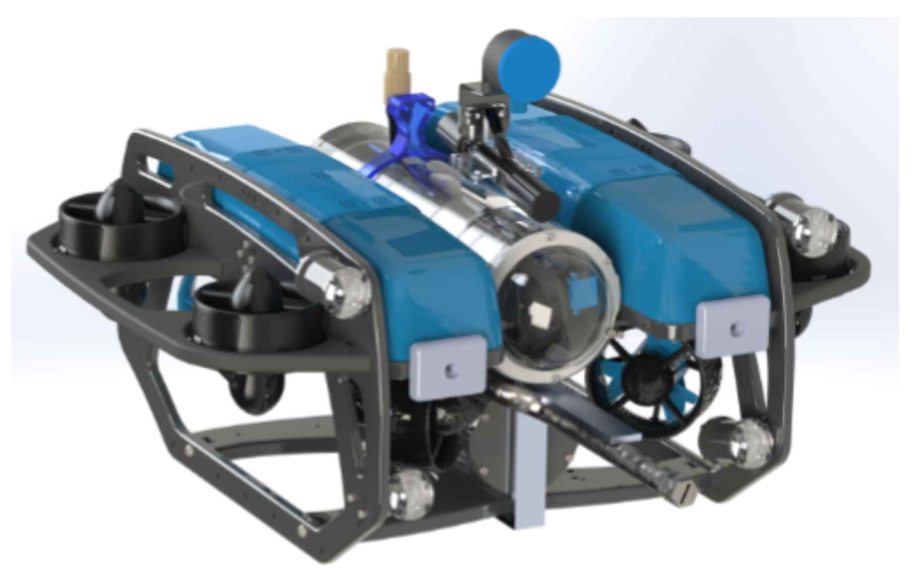
Previous studies [9] have shown that the acoustic positioning system used, which in this case was a short baseline (SBL) system, had varying time delay, which could not be handled properly by the suggested Smith-predictor. The impact of the delay has not been characterized, as the paper only concludes that the controller and Smith-predictor were not able to stabilize the ROV. This paper will evaluate how various time delays impact control performance. The range of time delays investigated is based on commonly used sensor technologies. The ROV used in this paper is the same being used in [15], which has been modified to perform cleaning operations using high-pressure water jetting. The modified ROV can be seen in Figure 1.

This paper will evaluate the effect of time delay ($\lambda$) and the maximum tolerated error ($ϵ$) on the output to quantify the effect on closed-loop performance. The study takes offset in a cleaning mission, where two different operation types are performed. These findings are used to give relevant values with regards to the parameters $\lambda$, which is the time delay introduced in the system by sensors or communication, and $e_{\mathit{max}}$, which is the maximum tolerated reference errors for the system. Two types of analysis are done to evaluate the system performance. First, a stability analysis is performed to investigate when and how the system becomes unstable. Then, an IO controllability analysis is given based on a model of the BlueROV2 and the chosen mission cases for quantifying the lower bounds of the unspecified optimal controllers’ performances. After the analysis, sensor technologies are evaluated concerning the results from the IO controllability analysis. This paper is finalized with a conclusion, which summarizes the quantitative analysis and sensor evaluation findings.

2. Cleaning Mission

When operating ROVs, the feedback and control system requirements can vary. Some operations require precise positioning meaning small errors and fast reaction time; such operations could be cleaning or welding operations. Other operations do not require the same small position errors but instead require reliable feedback for an extended period and distances; such operations could be navigation between members, where sub-meter precision is not as important.

The cleaning mission in this study will be concerning two different operations:

• A near-structure operation, where the ROV cleans underwater structures, such as risers, wells, or mono-piles.
• A off-structure navigation, where the ROV should navigate from one operation area to another, could be the vessel and the riser.

As seen in Figure 2, there will be switching between the near-structure operations and the off-structure navigation. The mission is done by first performing a off-structure navigation, where the ROV navigates from the vessel to the riser, followed by a near-structure operation. After finishing the near-structure operation, the ROV will perform a off-structure navigation navigating back to the vessel.

2.1. Near-Structure Operation

The near-structure operation is a cleaning operation, where high-pressure water jetting, like the one seen in Figure 3, is used to remove marine growth.

The quality of a “cleaning operation” depends on parameters such as the speed at which the water jet is moved relative to the structure, the pressure, and, lastly, the distance to the structure. Selecting these parameters is generally up to the skill of the operator. Yet, some experiments have been conducted by a project partner, which was conducted to find the most suitable cleaning tool for the project. The test was conducted in Port of Esbjerg using the setup seen in Figure 4.

The tests were conducted by moving high-pressure water jetting up and down against a wall with marine growth at multiple distances. The cleaning efficiency was then determined by visual inspection of the wall. The parameters affecting the cleaning efficiency can be seen in

Table 1. Parameters affecting cleaning efficiency.

Description	Parameter
Speed	$v_{cleaning}$ m/s
Water Pressure	$P_{jet}$ = 200 $\mathrm{bar}$
Distance to Structure where $ϵ$ is cleaning efficiency	$d_{cleaning}\in [0;0.1)m,ϵ=50\pm 10\%$ *
	$d_{cleaning}\in [0.1;0.2)\mathrm{m},ϵ=90\pm 5\%$ *
	$d_{cleaning}\in [0.2;0.3)\mathrm{m},ϵ=30\pm 10\%$ *
	$d_{cleaning}\in [0.3;\infty )m,ϵ=0\%$ *

^* The cleaning efficiency is based on visual observations, therefore these parameters are uncertain, however the values give a good impression on how the different distances impact the efficiency.

.

The ROV is self-stabilizing in roll and pitch orientation ($\varphi$ and $\theta$ respectively), which also has fixed control-reference at 0 degrees. Therefore these are not considered when determining the performance requirements for the two operations. The parameters used to define the control requirements are the maximum tolerated error $e_{\mathit{max}}={\left[\begin{array}{cccc}{e}_{max,N}& e_{max,E}& e_{max,D}& e_{max,\varphi }\end{array}\right]}^T$ and the maximum change of reference $r_{\mathit{max}}={\left[\begin{array}{cccc}{r}_{max,N}& r_{max,E}& r_{max,D}& r_{max,\varphi }\end{array}\right]}^T$.

From Table 1 it can be seen that the best range of operation is 0.1 m to 0.2 m; therefore, the lowest level of interest for errors in $e_{max,N}$ and $e_{max,E}$ are $0.2$ $\mathrm{m}$, to ensure the references could be set to $0.1$ $\mathrm{m}$ and operate in ranges, which results in some cleaning efficiency.

For D (down position in body frame), the errors are very depending on the purpose of cleaning. In some cases, only small points must be cleaned for inspection or welding, while cleaning a whole structure as part of a cleaning campaign results in more extensive operation areas. In this case, $0.5$ $\mathrm{m}$ is chosen as the maximum tolerated area, which means that only a small area is expected to be cleaned.

For $\psi$ (yaw orientation in body frame), the maximum changes would be $\frac{\pi }{2}$ rad as the pipe should be able to clean the pipe within this range. The maximum allowed error for $\psi$ is chosen to be 0.35 rad, as the water-jet should still be able to hit the pipe with this error.

2.2. Off-Structure Navigation

The ROV moves far from obstacles during the off-structure navigation, where the objective is motion between structures. In this type of operation, the state error is not as critical as the cleaning operation as long as the ROV reaches the structure. Therefore, the main goal is to reach a new operation area without a large drift in location. The distance between the vessel and the riser for this case study is 20 $\mathrm{m}$. When within a range of 1 $\mathrm{m}$ the ROV should be in the operating range for stereo vision as this is defined to be < 3 $\mathrm{m}$ in [16].

In summary, the following control performance parameters are chosen for near-structure operation and off-structure navigation (

Table 2. Control performance parameters for operations.

Parameter	Near-Structure Operation	Off-Structure Navigation
$e_{\mathit{max}}$	${\left[\begin{array}{cccc}0.2\mathrm{m}& 0.2\mathrm{m}& 0.5\mathrm{m}& 0.35\mathrm{rad}\end{array}\right]}^T$	${\left[\begin{array}{cccc}1\mathrm{m}& 1\mathrm{m}& 1\mathrm{m}& \frac{\pi }{2}\mathrm{rad}\end{array}\right]}^T$
$r_{\mathit{max}}$	${\left[\begin{array}{cccc}1\mathrm{m}& 1\mathrm{m}& 1\mathrm{m}& \frac{\pi }{2}\mathrm{rad}\end{array}\right]}^T$	${\left[\begin{array}{cccc}20\mathrm{m}& 20\mathrm{m}& 20\mathrm{m}& \pi \mathrm{rad}\end{array}\right]}^T$

).

2.3. Sensor Properties

To ensure reliable feedback for navigation different sensor types can be used. The sensors used on ROVs can be divided into three categories [17].

• Inertial/Dead reckoning
• Acoustic transponders/Absolute position
• Geophysical/Relative position

The inertial sensors such as the compass, Doppler Velocity Log (DVL), Inertial Measurement Unit (IMU), and pressure sensors are used to improve the dead reckoning estimation. Yet, such sensors can drift unbounded over time [17]. Therefore, additional sensors are needed to mitigate large navigation errors which accumulate over time.

The additional sensors could depend on the operation type.

2.3.1. Near-Structure Operation Sensors

For near-structure operations the pipe will be within visible range and visual odometry or visual simultaneous localization and mapping (SLAM) can mitigate the sensor-induced drift by dead-reckoning. Visual odometry relies on feature detection or filtering of video signals for determining motion or relative position [18]. The methods generally show the best performance when the surroundings are enriched with clear details. Consequently, the methods are more applicable when operating near-structure than during off-structure navigation.

2.3.2. Off-Structure Navigation Operation Sensors

Under off-structure navigation, the distance to a structure can be great; hence visual odometry might not work due to turbidity, and light decaying in water [18]. Therefore, acoustic transponders are traditionally used for mitigating drift effects. Yet, such sensors introduce a significant time delay in the feedback signal using the commercial Kalman Filter (KF) [8]. Experimental work has shown a varying time delay of 2.0 ± 0.5 s [9]. Another commonly used absolute positioning sensor is long baseline (LBL) system, which can have up to 10 s [19].

A disadvantage of using acoustic positing systems for operations near-structure could be decreased accuracy due to lack of line-of-sight between the transponder and the receivers [20].

In summary, the time delay, $\lambda$, will be evaluated up until 10 s or until the system is not stabilizable.

To be able to give quantitative evaluation on control performance for the different type of operations, a model of the used ROV has to be derived.

3. Modeling and Assumptions

The modeling is based on Fossen’s representation for underwater vehicles [21], and the parameters have been determined through a combination of experiments done in [15]. The details on the parameters can be found in the paper by Benzon et al. [15] where the same platform has been used.

The governing equations are given by:

$$\dot{\mathit{\eta }}=\mathit{J}\left(\mathit{\eta }\right)\mathit{\nu }$$

(1)

$$\mathit{M}\dot{\mathit{\nu }}+\mathit{C}\left(\mathit{\nu }\right)\mathit{\nu }+\mathit{D}\left(\mathit{\nu }\right)\mathit{\nu }+\mathit{g}\left(\mathit{\eta }\right)=\mathit{\tau }$$

(2)

where $\mathit{\eta }$ = ${\left[N,E,D,\varphi ,\theta ,\psi \right]}^T$ is a combination of world coordinates and Euler angles defined in the NED frame. $\mathit{\nu }$ = ${\left[u,v,w,p,q,r\right]}^T$ is the body-fixed velocity vector. The external forces $\mathit{\tau }={\left[{\mathit{\tau }}_1,{\mathit{\tau }}_2,{\mathit{\tau }}_3,{\mathit{\tau }}_4,{\mathit{\tau }}_5,{\mathit{\tau }}_6\right]}^T$ is the input given in force and torque. The rest of the variables in Equation (1) and (2) can be seen in

Table 3. Variables and their components.

Notation	Components
$\mathit{M}$	${\mathit{M}}_{\mathit{RB}}+{\mathit{M}}_{\mathit{A}}$
${\mathit{M}}_{\mathit{RB}}$	diag($m,m,m,I_x,I_y,I_z$)
${\mathit{M}}_{\mathit{A}}$	-diag($X_{\dot{u}},Y_{\dot{v}},Z_{\dot{w}},K_{\dot{p}},{\mathit{M}}_{\dot{q}},N_{\dot{r}}$)
$\mathit{C}$($\mathit{\nu }$)	$\left[\begin{array}{cc}\mathbf{0}& {\mathit{C}}_1\left(\mathit{\nu }\right)\\ {\mathit{C}}_2\left(\mathit{\nu }\right)& {\mathit{C}}_3\left(\mathit{\nu }\right)\end{array}\right]$
${\mathit{C}}_1$($\mathit{\nu }$)	$\left[\begin{array}{ccc}0& (m-Z_{\dot{w}})w& (Y_{\dot{v}}-m)v\\ (Z_{\dot{w}}-m)w& 0& (m-X_{\dot{u}})u\\ (m-Y_{\dot{v}})v& (X_{\dot{u}}-m)u& 0\end{array}\right]$
${\mathit{C}}_2$($\mathit{\nu }$)	$\left[\begin{array}{ccc}0& -(I_z+N_{\dot{r}})r& ({\mathit{M}}_{\dot{q}}-I_y)q\\ (N_{\dot{r}}+I_z)r& 0& (I_x-K_{\dot{p}})p\\ (I_y-{\mathit{M}}_{\dot{q}})q& (K_{\dot{p}}-I_x)p& 0\end{array}\right]$
$\mathit{D}$($\mathit{\nu }$)	-diag$\left(X_u\left(u\right),Y_v\left(v\right),Z_w\left(w\right),K_p\left(p\right),{\mathit{M}}_q\left(q\right),N_r\left(r\right)\right)$
$\mathit{g}$($\mathit{\eta }$)	$\left[\begin{array}{c}(W-B)sin\left(\theta \right)\\ -(W-B)cos\left(\theta \right)sin\left(\varphi \right)\\ -(W-B)cos\left(\theta \right)cos\left(\varphi \right)\\ y_{b}Bcos\left(\theta \right)cos\left(\varphi \right)-z_{b}Bcos\left(\theta \right)sin\left(\varphi \right)\\ -z_{b}Bsin\left(\theta \right)-x_{b}Bcos\left(\theta \right)cos\left(\varphi \right)\\ x_{b}Bcos\left(\theta \right)sin\left(\varphi \right)+y_{b}Bsin\left(\theta \right)\end{array}\right]$
W	$mg$
B	$\rho g\nabla$
${\mathit{J}}_1\left(\mathit{\eta }\right)$	${\left[\begin{array}{ccc}c\left(\psi \right)c\left(\theta \right)& c\left(\psi \right)s\left(\varphi \right)s\left(\theta \right)-c\left(\varphi \right)s\left(\psi \right)& s\left(\varphi \right)s\left(\psi \right)+c\left(\varphi \right)c\left(\psi \right)s\left(\theta \right)\\ c\left(\theta \right)s\left(\psi \right)& c\left(\varphi \right)c\left(\psi \right)+s\left(\varphi \right)s\left(\psi \right)s\left(\theta \right)& c\left(\varphi \right)s\left(\psi \right)s\left(\theta \right)-c\left(\psi \right)s\left(\varphi \right)\\ -s\left(\theta \right)& c\left(\theta \right)s\left(\varphi \right)& c\left(\varphi \right)c\left(\theta \right)\end{array}\right]}^{\ast }$
${\mathit{J}}_2\left(\mathit{\eta }\right)$	${\left[\begin{array}{ccc}1& s\left(\varphi \right)t\left(\theta \right)& c\left(\varphi \right)t\left(\theta \right)\\ 0& c\left(\varphi \right)& -s\left(\varphi \right)\\ 0& \frac{s\left(\varphi \right)}{c\left(\theta \right)}& \frac{c\left(\varphi \right)}{c\left(\theta \right)}\end{array}\right]}^{\ast }$
$\mathit{J}\left(\mathit{\eta }\right)$	$\left[\begin{array}{cc}{\mathit{J}}_1\left(\mathit{\eta }\right)& \mathbf{0}\\ \mathbf{0}& {\mathit{J}}_2\left(\mathit{\eta }\right)\end{array}\right]$

^*c = cos, s = sin, t = tan.

and

Table 4. Parameters used for the model, adapted from [15] with changed drag values.

Notation	Values/Term	Unit
g	9.82	m/s${}^2$
$\rho$	1000	$\mathrm{k}$$\mathrm{g}$/$\mathrm{m}$${}^3$
m	13.5	$\mathrm{k}\mathrm{g}$
∇	0.0133	${\mathrm{m}}^3$
$(I_x,I_y,I_z)$	(0.26, 0.23, 0.37)	$\mathrm{k}\mathrm{g}{\mathrm{m}}^2$
$(x_b,y_b,z_b)$	(0, 0, −0.01)	$\mathrm{m}$
$X_{\dot{u}}$	6.36	$\mathrm{k}\mathrm{g}$
$Y_{\dot{v}}$	7.12	$\mathrm{k}\mathrm{g}$
$Z_{\dot{w}}$	18.68	$\mathrm{k}\mathrm{g}$
$K_{\dot{p}}$	0.189	$\mathrm{k}\mathrm{g}{\mathrm{m}}^2$
${\mathit{M}}_{\dot{q}}$	0.135	$\mathrm{k}\mathrm{g}{\mathrm{m}}^2$
$N_{\dot{r}}$	0.222	$\mathrm{k}\mathrm{g}{\mathrm{m}}^2$
$X_u\left(u\right)$	$141\left|u\right|+13.7$	N s/m
$Y_v\left(v\right)$	$184\left|v\right|+20.0$ *	N s/m
$Z_w\left(w\right)$	$190\left|w\right|+33.0$	N s/m
$K_p\left(p\right)$	$0.95\left|p\right|+0.15$ *	N s
${\mathit{M}}_q\left(q\right)$	$0.47\left|q\right|+0.8$	N s
$N_r\left(r\right)$	$1.173\left|r\right|+0.2$ *	N s

^* The original drag terms found in [15] were Y_v(v) = 217|v|, K_p(p) = 1.19|p| and N_r(r) = 1.50|r|, however these have be redetermined to contain linear drag, this is elaborated in Section 4.

, which is also given in [15]. In Figure 5 both the North-East-Down (NED) (referred to as world frame as seen in Figure 5) and body-fixed frame definitions are shown.

The variables used in Table 3 can be seen in Table 4.

To get a mathematical expression of the acceleration, Equation (2) is solved as an inverse problem for $\dot{\mathit{\nu }}$.

$$\dot{\mathit{\nu }}={\mathit{M}}^{-1}\left(\mathit{\tau }-\mathit{C}\left(\mathit{\nu }\right)\mathit{\nu }-\mathit{D}\left(\mathit{\nu }\right)\mathit{\nu }-\mathit{g}\left(\mathit{\eta }\right)\right)$$

(3)

Equation (3) can then be formulated as a vector of non-linear functions.

$$\mathit{f}\left(\mathit{\eta },\mathit{\nu },\mathit{\tau }\right)={\left[\dot{u}\left(\mathit{\eta },\mathit{\nu },\mathit{\tau }\right),\dot{v}\left(\mathit{\eta },\mathit{\nu },\mathit{\tau }\right),\dot{w}\left(\mathit{\eta },\mathit{\nu },\mathit{\tau }\right),\dot{p}\left(\mathit{\eta },\mathit{\nu },\mathit{\tau }\right),\dot{q}\left(\mathit{\eta },\mathit{\nu },\mathit{\tau }\right),\dot{r}\left(\mathit{\eta },\mathit{\nu },\mathit{\tau }\right)\right]}^T$$

(4)

From Equation (3) and Table 3 it can noted that the non-linear model only depends on $\varphi$ and $\theta$ from $\mathit{\eta }$. As both of those is naturally zero do to restoring forces, they are set to zero in further modeling, and there is no intention to control the ROV’s orientation other than in heading. Therefore, $\mathit{f}\left(\mathit{\eta },\mathit{\nu },\mathit{\tau }\right)$ becomes $\mathit{f}\left(\mathit{\nu },\mathit{\tau }\right)$, where $\mathit{\nu }$ is the state matrix and $\mathit{\tau }$ is the input matrix.

4. Linearization and Reformulation

The non-linear model is linearized to suit the linear IO controllability analysis. For consistency, the velocity model is applied for linearization to avoid linearization of the rotation matrix.

The operation points chosen for linearization are different depending on the type of operation. During the near-structure operation, the ROV is mostly station-keeping and only slowly varies in both position and orientation; therefore, all states’ operation points are set to zero.

$${\mathit{OP}}_{\mathit{ns}}={\mathit{0}}_{6x1}$$

(5)

Recalling Table 4, it can be seen that the drag terms $Y_v\left(v\right)$, $K_p\left(p\right)$ and $N_r\left(r\right)$ has been modified to contain linear drag terms. The missing drag term found originally results in a deviation from the model even at small velocities; therefore, the three drag terms mentioned are redetermined with linear drag terms. The drag was originally found experimentally in [9]. However, the ROV used in this study was a standard configured BlueROV2, where this model is based on a modified BlueROV2 with heavy configuration. Therefore, some corrections have to be made. This was carried out by using the SolidWorks Flow Simulator to calculate the drag coefficients for the standard configured BlueROV2 and compare these results with the drag found experimentally. This comparison for sway motion can be seen in Figure 6.

The second-order fit is found by using the least-square method in Matlab’s Curve Fitting Toolbox and forcing the constant term to be 0, as no drag is present at zero velocity. polynomials for $Y_v\left(v\right)$ can be seen in

Table 5. 2nd order polynomials for $Y_v\left(v\right)$.

Data for Used for Fit	Polynomial
Simulation	$41.66\left|v\right|v$
Test	$\left(125.9\right|v|+7.364)v$
Simulation Corrected	$\left(41.66\right|v|+20)v$

.

The corrected fit for the simulation is found by using the quadratic drag term from the simulation fit and finding the linear drag term using both experimental data and simulation data. These corrections were used to calculate the drag terms for the modified BlueROV2 with heavy configuration, as shown in Figure 7.

In Figure 7, ‘2nd order fit’ = $50.94\left|v\right|v$ and ‘2nd order fit corrected’ = $\left(50.94\right|v|+20)v$.

Through experimental tests, the drag terms were then adjusted and became the values shown in Table 4. The adjustments made in the experimental validation removed the linear terms in $Y_v\left(v\right)$, $K_p\left(p\right)$ and $N_r\left(r\right)$. By reintroducing the linear terms and reducing the quadratic terms instead, the new drag terms can be seen in

Table 6. Drag terms used in this study, with refitted $Y_v\left(v\right)$, $K_p\left(p\right)$ and $N_r\left(r\right)$.

Notation	Values/Term	Unit
$X_u\left(u\right)$	$141\left|u\right|+13.7$	N s/m
$Y_v\left(v\right)$	$184.3\left|v\right|+20.0$	N s/m
$Z_w\left(w\right)$	$190\left|w\right|+33.0$	N s/m
$K_p\left(p\right)$	$0.95\left|p\right|+0.15$	N s
${\mathit{M}}_q\left(q\right)$	$0.47\left|q\right|+0.8$	N s
$N_r\left(r\right)$	$1.173\left|r\right|+0.2$	N s

.

During off-structure navigation, the ROV will be moving in all three translational directions. The velocity can vary; however, to find realistic operation points, the values in $O{P}_{os}$ are found by simulations, where the non-linear system is used with the controller described in Section 4.4. A reference change with the off-structure navigation values found in Table 2 is used, and maximum velocities for each direction are found. As roll and pitch do not have a reference, the initial conditions are changed to $\frac{\pi }{2}$ rad for each case, and the maximum velocity is then found.

$${\mathit{OP}}_{\mathit{os}}={\left[\begin{array}{cccccc}0.73\left(\frac{\mathrm{m}}{\mathrm{s}}\right)& 0.63\left(\frac{\mathrm{m}}{\mathrm{s}}\right)& 0.73\left(\frac{\mathrm{m}}{\mathrm{s}}\right)& 0.65\left(\frac{\mathrm{rad}}{\mathrm{s}}\right)& 0.88\left(\frac{\mathrm{rad}}{\mathrm{s}}\right)& 1.35\left(\frac{\mathrm{rad}}{\mathrm{s}}\right)\end{array}\right]}^T$$

(6)

As the forces applied to the system are modeled as a first-order variable, they will not affect the linearization and are set to 0 as operation points.

The linearization is done by utilizing the Jacobian method, first on states to get the state matrix.

$${\mathit{A}}_{\mathit{ns}}={\left.\frac{\partial \mathit{f}\left(\mathit{\nu },\mathit{\tau }\right)}{\partial \mathit{\nu }}\right|}_{\mathit{\nu }={\mathit{OP}}_{\mathit{ns}},\mathit{\tau }={\mathit{0}}_{6x1}}$$

(7)

$${\mathit{A}}_{\mathit{os}}={\left.\frac{\partial \mathit{f}\left(\mathit{\nu },\mathit{\tau }\right)}{\partial \mathit{\nu }}\right|}_{\mathit{\nu }={\mathit{OP}}_{\mathit{os}},\mathit{\tau }={\mathit{0}}_{6x1}}$$

(8)

and then on the input to get the input matrix.

$${\mathit{B}}_{\mathit{ns}}={\left.\frac{\partial \mathit{f}\left(\mathit{\nu },\mathit{\tau }\right)}{\partial \mathit{\tau }}\right|}_{\mathit{\nu }={\mathit{OP}}_{\mathit{ns}},\mathit{\tau }={\mathit{0}}_{6x1}}$$

(9)

$${\mathit{B}}_{\mathit{os}}={\left.\frac{\partial \mathit{f}\left(\mathit{\nu },\mathit{\tau }\right)}{\partial \mathit{\tau }}\right|}_{\mathit{\nu }={\mathit{OP}}_{\mathit{os}},\mathit{\tau }={\mathit{0}}_{6x1}}$$

(10)

As it has been assumed that full state feedback is available, the output matrix will be an identity matrix for both operation cases.

$$\mathit{C}={\mathit{I}}_{6x6}$$

(11)

Thereby the system can be expressed in state space.

$$\begin{array}{ccc}\dot{\mathit{\nu }}& =& \left\{\begin{array}{cc}{\mathit{A}}_{\mathit{ns}}\mathit{\nu }+{\mathit{B}}_{\mathit{ns}}\mathit{\tau }\hfill & \mathrm{if}\mathrm{near}-\mathrm{structure}\hfill \\ {\mathit{A}}_{\mathit{os}}\mathit{\nu }+{\mathit{B}}_{\mathit{os}}\mathit{\tau }\hfill & \mathrm{if}\mathrm{off}-\mathrm{structure}\mathrm{navigation}\hfill \end{array}\right.\hfill \\ \mathit{y}& =& \mathit{C}\mathit{\nu }\hfill \end{array}$$

(12)

where $\mathit{y}$ is the measured states.

4.1. Rewriting to Single-Input Single-Output Systems

When rewriting the state-space system into a SISO system, coupling between states cannot be considered, as this would require multiple outputs.

The linearization at ${\mathit{OP}}_{\mathit{off–structurenavigation}}$ results in a system:

$${\mathit{A}}_{\mathit{os}}=& \begin{array}{cc}\begin{array}{cccccc}\hfill u & v & w & p & q & r \end{array}& \\ \left[\begin{array}{cccccc}\hfill a_{1,1}& a_{1,2}& a_{1,3}\hfill & 0& a_{1,5}& a_{1,6}\\ \hfill a_{2,1}& a_{2,2}& a_{2,3}\hfill & a_{2,4}& 0& a_{2,6}\\ \hfill a_{3,1}& a_{3,2}& a_{3,3}\hfill & a_{3,4}& a_{3,5}& 0\\ \hfill 0& 0& 0\hfill & a_{4,4}& a_{4,5}& a_{4,6}\\ \hfill 0& 0& 0\hfill & a_{5,4}& a_{5,5}& a_{5,6}\\ \hfill 0& 0& 0\hfill & a_{6,4}& a_{6,5}& a_{6,6}\end{array}\right]& \begin{array}{c}u\\ v\\ w\\ p\\ q\\ r\end{array}\end{array}$$

(13)

For linearization at ${\mathit{OP}}_{\mathit{near–structure}}$, the A matrix is similar to ${\mathit{A}}_{\mathit{os}}$, but with no coupling terms. The coupling terms are defined as all entries that do not lie on the diagonal.

The input matrix $\mathit{f}\left({\mathit{x}}_{\mathit{state}}\right)$ is given as:

$${\mathit{B}}_{\mathit{ns}}={\mathit{B}}_{\mathit{os}}=\begin{array}{cc}\begin{array}{cccccc}\hfill {\tau }_1 & {\tau }_2 & {\tau }_3 & {\tau }_4 & {\tau }_5 & {\tau }_6 \end{array}& \\ \left[\begin{array}{cccccc}\hfill b_{1,1}& 0& 0\hfill & 0& 0& 0\\ \hfill 0& b_{2,2}& 0\hfill & 0& 0& 0\\ \hfill 0& 0& b_{3,3}\hfill & 0& 0& 0\\ \hfill 0& 0& 0\hfill & b_{4,4}& 0& 0\\ \hfill 0& 0& 0\hfill & 0& b_{5,5}& 0\\ \hfill 0& 0& 0\hfill & 0& 0& b_{6,6}\end{array}\right]& \begin{array}{c}u\\ v\\ w\\ p\\ q\\ r\end{array}\end{array}$$

(14)

In

Table 7. Entries for state matrix ($A_{os}$ and $A_{ns}$ and input matrix ($B_{os}$ and $B_{ns}$).

Entry	Aos	Ans	Entry	Aos	Ans	Entry	Aos	Ans	Entry	Aos	Ans	Entry	Bos & Bns
$a_{1,1}$	−11.11	−0.69	$a_{2,2}$	−12.22	−0.97	$a_{3,3}$	−9.59	−1.03	$a_{5,4}$	0.54	0.00	$b_{1,1}$	0.05
$a_{1,2}$	2.20	0.00	$a_{2,3}$	0.63	0.00	$a_{3,4}$	−0.39	0.00	$a_{5,5}$	−4.47	−2.19	$b_{2,2}$	0.05
$a_{1,3}$	−0.92	0.00	$a_{2,4}$	0.70	0.00	$a_{3,5}$	0.47	0.00	$a_{5,6}$	0.26	0.00	$b_{3,3}$	0.03
$a_{1,5}$	−0.75	0.00	$a_{2,6}$	−1.15	0.00	$a_{4,4}$	−3.11	−0.34	$a_{6,4}$	0.12	0.00	$b_{4,4}$	2.24
$a_{1,6}$	1.02	0.00	$a_{3,1}$	0.57	0.00	$a_{4,5}$	−0.69	0.00	$a_{6,5}$	0.09	0.00	$b_{5,5}$	2.74
$a_{2,1}$	−2.11	0.00	$a_{3,2}$	−0.40	0.00	$a_{4,6}$	−0.45	0.00	$a_{6,6}$	−5.71	−0.34	$b_{6,6}$	1.69

the $a_{i,j}$ terms calculated using Equations (7) and (8) and the $b_{i,i}$ terms calculated from (9) and (10) can be seen.

It can be noted that the input matrix is independent of the operation points.

From the state-space model, a matrix of SISO systems can easily be derived using the general formulation:

$${\mathit{G}}_{\mathit{ol}}\left(s\right)=\mathit{C}{(sI-\mathbf{A})}^{-1}\mathbf{B}$$

(15)

${\mathit{G}}_{\mathit{ol}}$ is a transfer function matrix.

There will only be one transfer function for each input when no coupling terms are considered, which is the transfer function from $\mathit{\tau }$ to the state in each degree-of-freedom (DOF).

$${\mathit{G}}_{\mathit{ol}}\left(s\right)=\left[\begin{array}{cccccc}{G}_{ol,u,{\mathit{\tau }}_1}\left(s\right)& G_{ol,u,{\mathit{\tau }}_2}\left(s\right)& G_{ol,u,{\mathit{\tau }}_3}\left(s\right)& G_{ol,u,{\mathit{\tau }}_4}\left(s\right)& G_{ol,u,{\mathit{\tau }}_5}\left(s\right)& G_{ol,u,{\mathit{\tau }}_6}\left(s\right)\\ G_{ol,v,{\mathit{\tau }}_1}\left(s\right)& G_{ol,v,{\mathit{\tau }}_2}\left(s\right)& G_{ol,v,{\mathit{\tau }}_3}\left(s\right)& G_{ol,v,{\mathit{\tau }}_4}\left(s\right)& G_{ol,v,{\mathit{\tau }}_5}\left(s\right)& G_{ol,v,{\mathit{\tau }}_6}\left(s\right)\\ G_{ol,w,{\mathit{\tau }}_1}\left(s\right)& G_{ol,w,{\mathit{\tau }}_2}\left(s\right)& G_{ol,w,{\mathit{\tau }}_3}\left(s\right)& G_{ol,w,{\mathit{\tau }}_4}\left(s\right)& G_{ol,w,{\mathit{\tau }}_5}\left(s\right)& G_{ol,w,{\mathit{\tau }}_6}\left(s\right)\\ 0& 0& 0& G_{ol,p,{\mathit{\tau }}_4}\left(s\right)& G_{ol,p,{\mathit{\tau }}_5}\left(s\right)& G_{ol,p,{\mathit{\tau }}_6}\left(s\right)\\ 0& 0& 0& G_{ol,q,{\mathit{\tau }}_4}\left(s\right)& G_{ol,q,{\mathit{\tau }}_5}\left(s\right)& G_{ol,q,{\mathit{\tau }}_6}\left(s\right)\\ 0& 0& 0& G_{ol,r,{\mathit{\tau }}_4}\left(s\right)& G_{ol,r,{\mathit{\tau }}_5}\left(s\right)& G_{ol,r,{\mathit{\tau }}_6}\left(s\right)\end{array}\right]$$

(16)

For the linearized system at off-structure navigation ${\mathit{G}}_{\mathit{ol,os}}\left(s\right)$, some coupling terms are present; these are seen in the presence of transfer functions that lie outside the diagonal.

4.2. Coupling Effect Analysis

The coupling effects for the off-structure navigation system are investigated through Relative Gain Array (RGA) analysis. RGA is a method used to determine the interaction between inputs and outputs as done [22], which can be seen in extended form in [23].

The RGA matrix is defined by:

$$\Lambda \left({\mathit{G}}_{\mathit{ol,os}}\left(s\right)\right)={\mathit{G}}_{\mathit{ol,os}}\left(s\right)\circ {\left({\mathit{G}}_{\mathit{ol,os}}{\left(s\right)}^{-1}\right)}^T$$

(17)

where ∘ is the Hadamard product, also known as element-wise product.

RGA analysis is often evaluated at steady-state (s = 0) to provide steady-state behavior [22].

The steady-state values for the RGA matrix are:

$$\Lambda \left({\mathit{G}}_{\mathit{ol,ov}}\left(0\right)\right)=\begin{array}{cc}\begin{array}{cccccc}\hfill {\tau }_1& {\tau }_2 & {\tau }_3 & {\tau }_4 & {\tau }_5 & {\tau }_6 \end{array}& \\ \left[\begin{array}{cccccc}\hfill 0.96& 0.03& 0.01\hfill & 0& 0& 0\\ \hfill 0.03& 0.97& 0.00\hfill & 0& 0& 0\\ \hfill 0.01& 0.00& 0.99\hfill & 0& 0& 0\\ \hfill 0& 0& 0\hfill & 0.98& 0.02& 0\\ \hfill 0& 0& 0\hfill & 0.02& 0.98& 0\\ \hfill 0& 0& 0\hfill & 0& 0& 1\end{array}\right]& \begin{array}{c}u\\ v\\ w\\ p\\ q\\ r\end{array}\end{array}$$

(18)

The dominating part is the diagonal gains for all directions, which is clearly seen by the entries in Equation (18). However, the cross interaction between the inputs and outputs is still present in the actual system. It is also seen that the input for a certain DOF is the best choice of actuation for this DOF.

It must be noted that the coupling is more dominant when the velocity rises. At maximum velocity, entry 1,1 goes down to 0.73 from 0.96.

Another notable thing in terms of coupling is that the thrusters can provide force and torque for a single DOF. This is only the case if they are precisely placed in regard to the center of mass (COM), which can be hard to achieve in a physical system.

4.3. Padé Approximation

The (IO controllability) can only be applied for a rational transfer function. Time delays are infinite-dimensional systems and must therefore be approximated to a rational transfer function [14]. Different approximations exist for making time delays rational functions, these include Taylor expansion, and Páde approximation [24]. To keep the approximation simple, a first-order approximation is used. For first-order approximations, Taylor expansion and Páde approximation are the same.

Consider the following transfer function matrix:

$$G_{ol}^{delayed}\left(s\right)=G_{ol}\left(s\right){\mathrm{e}}^{-\mathrm{s}\lambda }$$

(19)

Here, the first-order Páde approximation is:

$$e^{-\mathrm{s}\lambda }\approx \frac{-s+\frac{2}{\lambda }}{s+\frac{2}{\lambda }}$$

(20)

By combining Equations (19) and (20) the time delay is replaced with a pole and a zero.

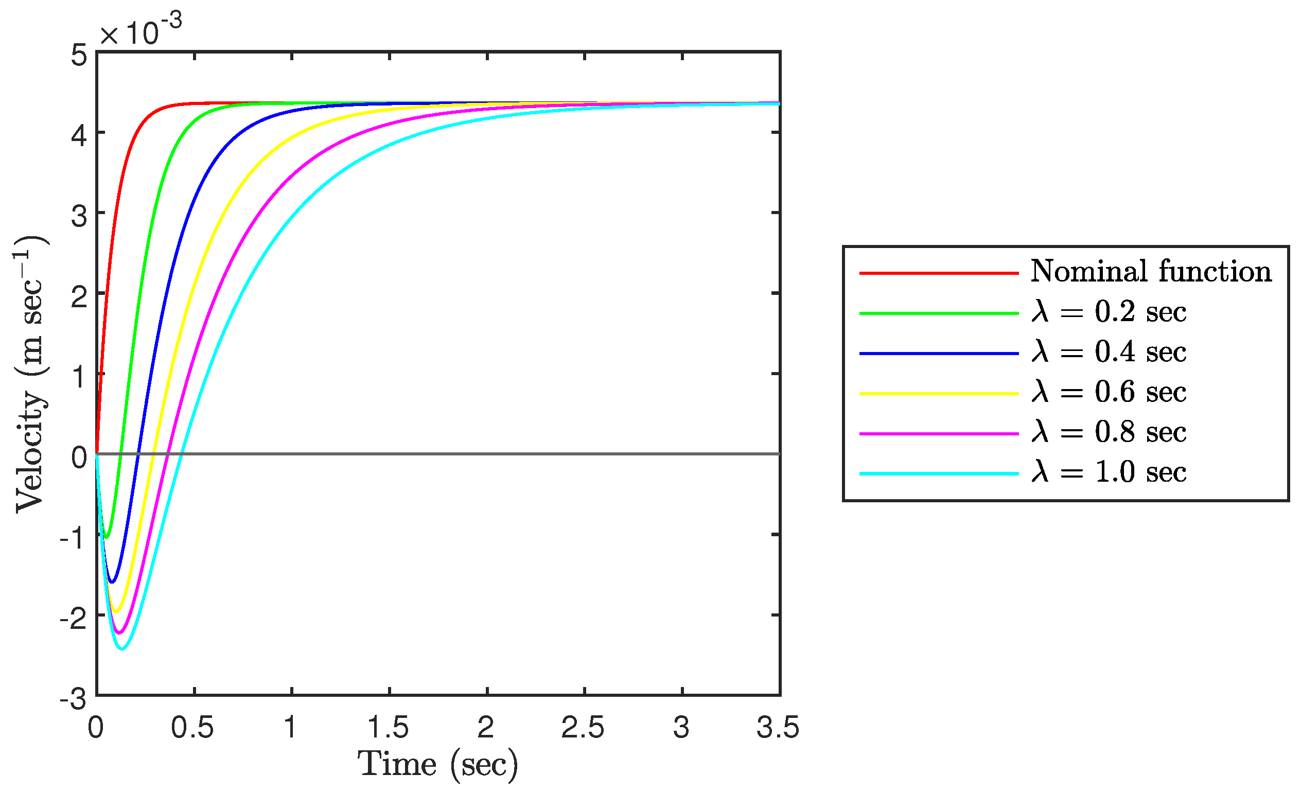
In Figure 8, it can be seen that Padé approximation results in an inverse response when given a step input. The inverse response is expected due to the added RHP zero, resulting in a non-minimum phase system. The introduced inverse response makes the Padé approximation deviate from a pure time delay.

It is noted that the steady-state gradient is independent of the time delay. Hence, the steady-state velocities reach the same steady-state equilibrium independent of the Padé approximation.

It can also be noted that the system $G_{ol}$ is observable, controllable, and stable for all time delays and operation points.

4.4. Nominal Closed-Loop System

In [15] a linear quadratic regulator with integral action (LQRI) is designed for a nominal system without time delay. This study will implement the same controller as a new open-loop system with reference as input. Then the IO controllability analysis is then used to find the maximum possible time delay at which the system shows acceptable control performance by applying a new controller to the new open-loop system. More simply this can be seen as a reconfiguration of the existing controller. In other words the IO controllability is used to evaluate the control performance of the best possible reconfiguration of the existing controller.

Another approach to solving the time delay problem could be developing an Internal Model Control (IMC) as proposed in [25] or developing a robust controller that can handle variable parameter changes such as time delays [11].

However, as mentioned in Section 2.3, time delays can vary; therefore, it is not possible to identify the time delay online. Analysis of the maximum possible time delay for a certain closed-loop system could also support finding correct properties for new sensors for an existing system with feedback control in place.

The LQRI used in the analysis is designed in [15]. The LQRI is designed for a MIMO system; therefore, it has to be rewritten for the SISO-systems derived in Section 4.1.

The gains for the LQRI controller used in [15] are:

$$\mathit{K}=\left[\begin{array}{cccccccccccc}113.15& 26.85& 0& 0& 0& 0& 0& 0& 0& 0& 0& 0\\ 0& 0& 131.84& 15.75& 0& 0& 0& 0& 0& 0& 0& 0\\ 0& 0& 0& 0& 209.14& 33.19& 0& 0& 0& 0& 0& 0\\ 0& 0& 0& 0& 0& 0& 0.67& 1.07& 0& 0& 0& 0\\ 0& 0& 0& 0& 0& 0& 0& 0& 0.71& 0.74& 0& 0\\ 0& 0& 0& 0& 0& 0& 0& 0& 0& 0& 14.94& 2.97\end{array}\right]$$

(21)

$${\mathit{K}}_{\mathit{i}}=\left[\begin{array}{cccc}45.56& 0& 0& 0\\ 0& 49.94& 0& 0\\ 0& 0& 103.52& 0\\ 0& 0& 0& 0\\ 0& 0& 0& 0\\ 0& 0& 0& 18.84\end{array}\right]$$

(22)

It can be seen that each control input only depends on a single direction’s velocity, position, and integrated position. Therefore the LQRI can easily be transformed into a proportional–integral–derivative (PID) controller.

Recall Equation (12):

$$\dot{\mathit{x}}\left(s\right)=\mathit{A}\mathit{x}\left(s\right)+\mathit{B}\mathit{\tau }\left(s\right)$$

(23)

$$\mathit{\tau }\left(s\right)={\mathit{K}}_{\mathit{i}}\frac{1}{s}\left({\mathit{u}}_r\left(s\right)-{\mathit{\eta }}_c\left(s\right)\right)-\mathit{K}\mathit{x}\left(s\right)$$

(24)

where ${\mathit{u}}_{\mathit{r}}$(s) is a 4 by 1 vector ${[u_N\left(s\right),u_E\left(s\right),u_D\left(s\right),u_{\psi }\left(s\right)]}^T$ with the desired position in surge, sway, heave and yaw direction respectively. ${\mathit{\eta }}_{\mathit{c}}\left(s\right)$ is the positions and orientation of interest, here presented as anti-derivative of $\mathit{\nu }\left(s\right)$ in surge, sway, heave and yaw direction,

$${\mathit{\eta }}_{\mathit{c}}\left(s\right)={\left[\frac{u\left(s\right)}{s},\frac{v\left(s\right)}{s},\frac{w\left(s\right)}{s},\frac{r\left(s\right)}{s}\right]}^T$$

(25)

$\mathit{x}$(s) is combination of $\mathit{\nu }\left(s\right)$ and its anti-derivative.

$$\mathit{x}\left(s\right)={\left[\frac{u\left(s\right)}{s},u\left(s\right),\frac{v\left(s\right)}{s},v\left(s\right),\frac{w\left(s\right)}{s},w\left(s\right),\frac{p\left(s\right)}{s},p\left(s\right),\frac{q\left(s\right)}{s},q\left(s\right),\frac{r\left(s\right)}{s},r\left(s\right)\right]}^T$$

(26)

As seen in Equation (25) there are no reference for $\varphi$ and $\theta$. It is observed that these orientations have strong self-stabilizing properties at 0 ${}^{\circ }$, and as the desired values for these are constantly 0 ${}^{\circ }$, these have been neglected for simplicity.

An example of the procedure for rewriting the LQRI to PID is done for a single DOF but is the same for the four DOFs, which have a desired reference.

$${\mathit{\tau }}_1\left(s\right)=K_i(1,1)\frac{1}{s}\left(u_N\left(s\right)-N\left(s\right)\right)-\left(K\left(1,1\right)N\left(s\right)+K\left(2,1\right)sN\left(s\right)\right)$$

(27)

Then Equation (27) can be written into transfer function $G_{ol,N,{\mathit{\tau }}_1}\left(s\right)$ seen in Equation (16).

$$G_{N,u_N}\left(s\right)=\frac{N\left(s\right)}{{\mathit{\tau }}_1\left(s\right)}{\mathit{\tau }}_1\left(s\right)=\frac{N\left(s\right)}{u_N\left(s\right)}$$

(28)

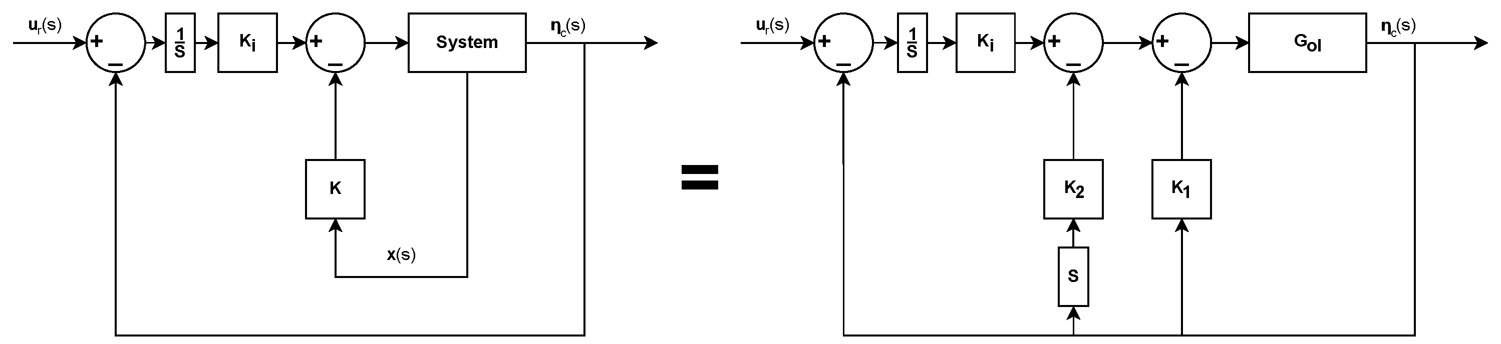
By following a similar procedure for surge, sway, heave and yaw a four by four transfer matrix G of the nominal closed-loop system is derived.

$$\mathbf{G}\left(s\right)=\left[\begin{array}{cccc}{G}_{N,u_N}\left(s\right)& 0& 0& 0\\ 0& G_{E,u_E}\left(s\right)& 0& 0\\ 0& 0& G_{D,u_D}\left(s\right)& 0\\ 0& 0& 0& G_{\psi ,u_{\psi }}\left(s\right)\end{array}\right]$$

(29)

${\mathit{K}}_{\mathit{1}}$ in Figure 9 is the odd columns in $\mathit{K}$ seen in Equation (21) and $\mathit{K}$ is the even columns in $\mathit{K}$.

4.5. Scaling

Scaling is performed by normalizing the system inputs and outputs which is required for IO controllability analysis [14]. In- and output scaling is performed according to:

$${\mathit{G}}_{\mathit{scaled}}\left(s\right)={{\mathit{D}}_{\mathit{e}}}^{-1}\mathit{G}\left(s\right){\mathit{D}}_{\mathit{u}}$$

(30)

${\mathit{D}}_{\mathit{e}}$ is the output scale vector, ${\mathit{D}}_{\mathit{u}}$ is the input scale vector.

The outputs are scaled based on the largest allowed controlled error ${\mathit{e}}_{\mathit{max}}$ and found based on the findings summarized in Table 2.

$${\mathit{D}}_{\mathit{e,ns}}={\mathit{e}}_{\mathit{max,ns}}={\left[0.20.20.50.35\right]}^T$$

(31)

$${\mathit{D}}_{\mathit{e,os}}={\mathbf{e}}_{\mathit{max,os}}={\left[111\frac{\pi }{2}\right]}^T$$

(32)

${\mathit{D}}_{\mathit{r}}$ is the maximum expected change in reference. It is designed differently for near-structure and off-structure navigation, as the maximum references changes are different depending on the type of operation. The values chosen can be seen in Table 2.

As mentioned in Section 2, near-structure operations normally requires precise position for effective operation, therefore the reference changes are also expected to be small while performing the near-structure operations.

$${\mathit{D}}_{\mathit{r,ns}}={\mathit{r}}_{\mathit{max,ns}}={\left[111\frac{\pi }{2}\right]}^T$$

(33)

For off-structure navigation the task can be moving from one riser to another, or traveling from and to the service vessel, which can be tenth of meters away from the riser, therefore the reference changes will also be significantly larger than for near-structure operation.

$${\mathit{D}}_{\mathit{r,os}}={\mathit{r}}_{\mathit{max,os}}={\left[202020\pi \right]}^T$$

(34)

${\mathit{D}}_{\mathit{u}}$ is the maximum allowed input change, this depends typically on the actuators’ limits, but in this case, $\mathit{G}$(s) is the nominal closed-loop system, meaning that the input is not directly associated with the maximum thrust. As the nominal closed-loop system has a dc-gain at 1 for all directions, the input should be scaled in relation to the references.

As the output and the reference are scaled according to ${\mathit{D}}_{\mathit{r}}$, ${\mathit{D}}_{\mathit{u}}$ should be the inverse.

$${\mathit{D}}_{\mathit{u,ns}}={\mathit{D}}_{\mathit{r,ns}}^{-1}$$

(35)

$${\mathit{D}}_{\mathit{u,os}}={\mathit{D}}_{\mathit{r,os}}^{-1}$$

(36)

Finally, the scaling of the system yields:

$${\mathit{G}}_{\mathit{scaled,ns}}\left(s\right)={\mathit{D}}_{\mathit{e,ns}}^{-1}{\mathit{G}}_{\mathit{ns}}\left(s\right){\mathit{D}}_{\mathit{u,ns}}$$

(37)

$${\mathit{G}}_{\mathit{scaled,os}}\left(s\right)={\mathit{D}}_{\mathit{e,os}}^{-1}{\mathit{G}}_{\mathit{os}}\left(s\right){\mathit{D}}_{\mathit{u,os}}$$

(38)

This results in two normalized system ${\mathit{G}}_{\mathit{scaled,ns}}$(s) and ${\mathit{G}}_{\mathit{scaled,os}}$(s).

5. Model Analysis

The model analysis is divided into a stability analysis followed by an input-output controllability analysis. The stability analysis is a conventional system stability analysis, which determines whether a system is stable based on the poles. Section 5.2 presents an input-output controllability analysis to quantify the ability to achieve acceptable control performance for the unstable system given the requirements implicitly issued by the scaling operations in Section 4.5.

The system of interest for these analysis is ${\mathit{G}}_{\mathit{scaled,ns}}^{\mathit{delayed}}\left(s\right)$ and ${\mathit{G}}_{\mathit{scaled,os}}^{\mathit{delayed}}\left(s\right)$, recall that the time delay, $\lambda$, is investigated up until 10 s, however for this analysis it will not be further investigated, when the system becomes unstable.

5.1. Performance Analysis on Stable Region

The nominal closed-loop systems stabilities are investigated in regards to different time delays by investigating the pole placement. When the poles are located in the RHP, the system becomes unstable. As a higher time delay moves the poles in the right direction, eventually, the system becomes unstable. In

Table 8. Maximum time delay for stable nominal closed-loop system.

Direction	Near-Structure Operation	Off-Structure Navigation
$G_{scaled,N,u_N}^{delayed}\left(s\right)$	0.28 s	1.94 s
$G_{scaled,E,u_E}^{delayed}\left(s\right)$	0.21 s	1.87 s
$G_{scaled,D,u_D}^{delayed}\left(s\right)$	0.24 s	1.44 s
$G_{scaled,\psi ,u_{\psi }}^{delayed}\left(s\right)$	0.17 s	0.43 s

the time delay at which the nominal closed-loop systems are stable has been found and can be seen.

Off-structure navigation is generally seen to allow for increased time delays when compared to near-structure operation. This follows intuition, as the motion during off-structure navigation occurs at higher velocities and, thus, is associated with an increase in damping induced by drag.

Another interesting thing to evaluate is the closed-loop performance, one way to evaluate this is by computing the integrated absolute error (IAE) of the control error $\mathit{e}={\mathit{\eta }}_c-{\mathit{u}}_r$ as done in [26].

For a single system, IAE can be computed by.

$$\mathrm{IAE}={\int }_0^{\infty }\left|e\left(t\right)\right|dt$$

(39)

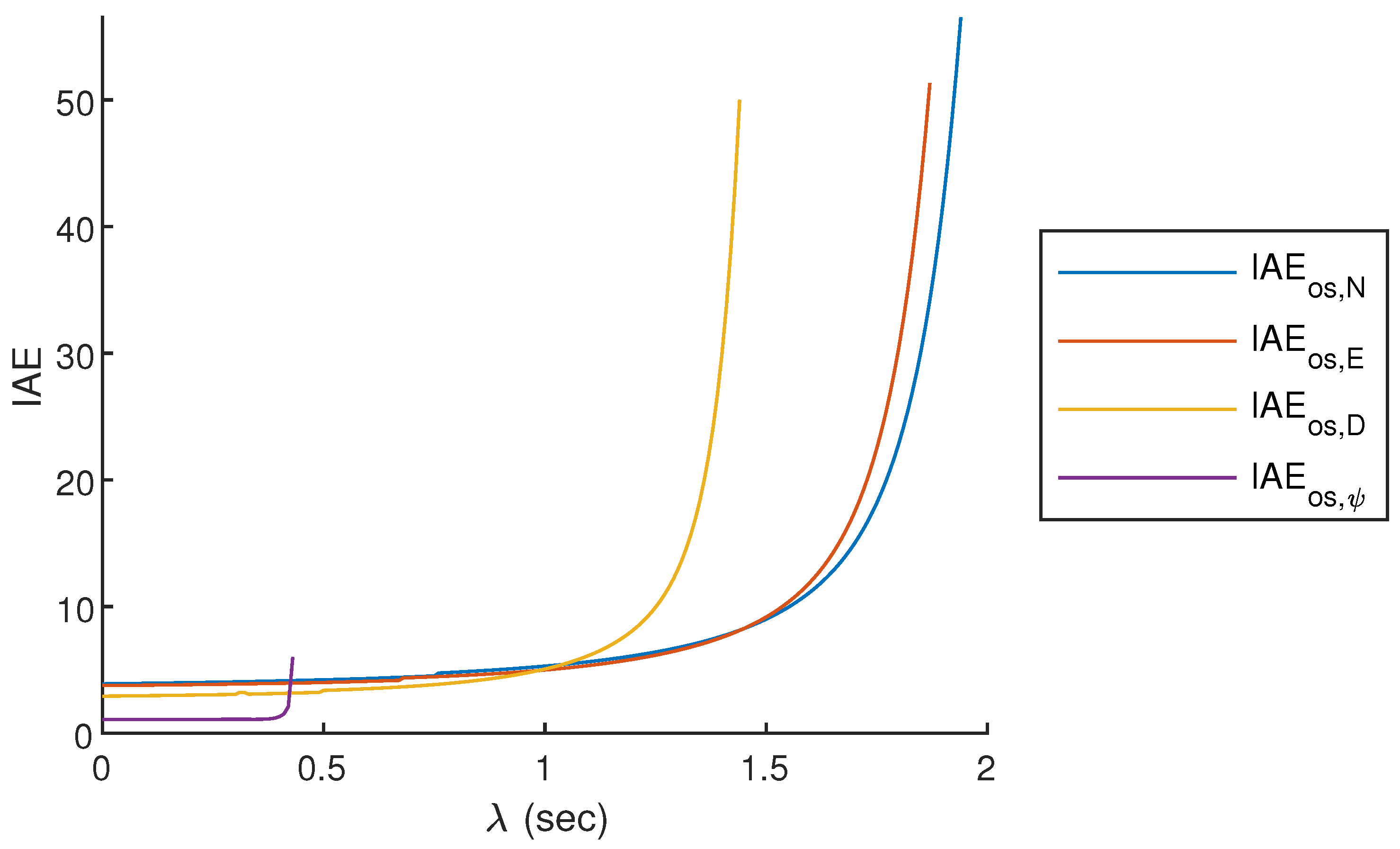
When the system becomes unstable IAE $\to \infty$ as $t\to \infty$, therefore unstable systems has not been considered for the output performance evaluation, the results can be seen in Figure 10 and Figure 11.

As seen from Figure 10 and Figure 11, the change in IAE is more rapid for near-structure operation, meaning that a slight change in time delay results in poor output performance. Another observation is that even though off-structure navigation tolerates extensive delays, the output performance becomes very poor at extensive time delays; therefore, these should be avoided.

The output performance is evaluated on a system that is not affected by disturbances. However, in real operations, the ROV is exposed to disturbances from the tether, current, waves, and the water jet, which will result in decreased output performances.

The nominal closed-loop systems are evaluated through IO controllability analysis to investigate whether the systems can be redesigned to allow larger time delays.

5.2. Input-Output Controllability Analysis

Controllability is defined as the ability to achieve acceptable control performance. IO Controllability is used to find what control performance can be expected by a closed-loop system without defining control parameters. Commonly, a simulation approach is used. However, this approach requires that the controller is specified and limits the results in a general sense [14].

The IO Controllability is used to quantify the controllability of the system by evaluating the minimum achievable peaks of different transfer functions. The calculations of these peaks are dependent on the location of the poles and zeros of the open-loop system. For the controllability analysis, it is assumed, that model is defined by $y=G\left(s\right)u+G_d\left(s\right)d$ with a control design $u=K\left(s\right)(r-y-n)$. Here d is the disturbances, n is the measurement noise and r is the reference setpoint [26]. In this study, the disturbances are neglected; therefore, the system model is defined as $y=G\left(s\right)u$, this form is shown in Figure 12.

The closed-loop system can be presented as,

$$y\left(j\omega \right)=T\left(j\omega \right)r\left(j\omega \right)-T\left(j\omega \right)n\left(j\omega \right)$$

(40)

where $T\left(j\omega \right)$ is the complementary sensitivity function.

$$T\left(j\omega \right)=G\left(j\omega \right)K\left(j\omega \right){(I+G\left(j\omega \right)K\left(j\omega \right))}^{-1}$$

(41)

The control input can then be defined as:

$$u\left(j\omega \right)=K\left(j\omega \right)S\left(j\omega \right)\left(r\right(j\omega )-n(j\omega \left)\right)$$

(42)

where $S\left(j\omega \right)$ is the sensitivity function,

$$S\left(j\omega \right)={(I+G\left(j\omega \right)K\left(j\omega \right))}^{-1}$$

(43)

The transfer functions of interest in IO Controllability analysis are S, T, $KS$ and $SG$, which can be seen as measures of robustness against different types of uncertainty. The “peak” is the maximum value of $H_{\infty }$ norm,

$${\mathit{M}}_S=\underset{0\le \omega \le \infty }{max}\left|\left|S\left(j\omega \right)\right|\right|$$

(44)

which is also the peak of the transfer function. The bounds are not dependent on the controller K, but physical properties of the system G. However, the bounds are dependent on correct scaling of the system, which is shown in Section 4.5.

The peak is closely related to the gain margin (GM) and phase margin (PM), as given ${\mathit{M}}_s$ guaranteed a certain GM and PM [14].

$$G\mathit{M}\ge \frac{{\mathit{M}}_S}{{\mathit{M}}_S-1}$$

(45)

$$P\mathit{M}\ge 2\mathrm{asin}\left(\frac{1}{2{\mathit{M}}_S}\right)\ge \frac{1}{{\mathit{M}}_S}\left(rad\right)$$

(46)

5.2.1. Lower Bound on S

The lowest achievable peak values for S and T, ${\mathit{M}}_{S,min}$ and ${\mathit{M}}_{T,min}$ are calculated based on the distance between the unstable poles ($p_i$) and zero (z) of the open-loop system:

$$\underset{K}{min}{\left|\right|S\left(j\omega \right)\left|\right|}_{\infty }\ge {\mathit{M}}_{S,min}=\prod _{i=1}^{N_p}\frac{|z+p_i|}{|z-p_i|}$$

(47)

${\mathit{M}}_{S,min}$ is used to determine whether a system is stable or not, if ${\mathit{M}}_{S,min}>1$ then a controller is needed to stabilize the system. For good performance ${\mathit{M}}_{S,min}$ typically needs to be smaller than 2 and ${\mathit{M}}_{S,min}>4$ indicates poor performance and poor robustness [14].

5.2.2. Lower Bound on KS

The function describing $KS$ is a transfer function from n to u, and hence considers the effect of the measurement noise and output disturbances. The lowest peak of $KS$ is estimated according to:

$${\left|\right|KS\left|\right|}_{\infty }\ge \left|G_s{\left(p\right)}^{-1}\right|$$

(48)

where $G_s$ is a stable transfer function where the RHP-poles of G is mirrored into the LHP. When there are multiple and complex unstable poles the peak can be calculated as:

$${\left|\right|KS\left|\right|}_{\infty }\ge \frac{1}{{\underline{\sigma }}_H}\left(U{\left(G\right)}^{\ast }\right)$$

(49)

where ${\underline{\sigma }}_H$ is the smallest Hankel singular value and $U{\left(G\right)}^{\ast }$ is the mirrored image of the antistable part of G.

For some of the systems ${\mathit{G}}_{\mathit{scaled,ns}}^{\mathit{delayed}}(s,\lambda )$ and ${\mathit{G}}_{\mathit{scaled,os}}^{\mathit{delayed}}(s,\lambda )$, the complex unstable poles converts into two unstable poles on the real axis, when $\lambda$ gets sufficiently large. As the calculation is only valid for cases with two complex poles, ${\left|\right|KS\left|\right|}_{\infty }$ is not calculated beyond this point.

5.2.3. Lower Bound on SG

$SG$ relates to the input disturbances and robustness against pole uncertainty, this includes uncertainty of the time delay. For any single unstable zero, denoted as z, the lower boundaries of the $H_{\infty }$ norms of the transfer functions for $SG$ can be estimated according to:

$${\left|\right|SG\left|\right|}_{\infty }\ge \left|G_{ms}\left(z\right)\right|\prod _{i=1}^{N_p}\frac{z+p_i}{z-p_i}$$

(50)

where $G_{ms}$ is the minimum phase stable version of G as both RHP poles and zeros are mirrored into the LHP.

All transfer functions are calculated for the systems ${\mathit{G}}_{\mathit{scaled,ns}}^{\mathit{delayed}}\left(s\right)$ and ${\mathit{G}}_{\mathit{scaled,os}}^{\mathit{delayed}}\left(s\right)$ for $\lambda$ up to until the ${\mathit{M}}_{S,min}$ crosses 4 as this defined as the upper control limit.

5.3. Analytical Results

The results are presented for each of the four controlled DOFs for both near-structure and off-structure navigation.

It is worth knowing that the included figures’ axes are scaled for readability and, therefore, might vary between the figures.

5.3.1. Lower Bound for S

Recall that ${\parallel S\parallel }_{\infty ,min}$ has to be 4, and preferably also smaller than 2. These two bounds are shown on Figure 13 and Figure 14 as Upper Control Limit (UCL) and Lower Control Limit (LCL), respectively. A selection of values is also shown in

Table 9. Selected values for ${\parallel S\parallel }_{\infty ,min}$.

$\mathit{\lambda }\left[\mathbf{s}\right]$	0.00	0.60	1.20	1.80	2.40	3.00	3.60	4.20	4.80	5.40	6.00
Near-structure operation
N [$\mathrm{m}$]	1.00	1.73	3.90	6.77	10.28	14.41	19.15	24.49	30.43	36.96	44.08
E [$\mathrm{m}$]	1.00	1.83	3.84	6.43	9.51	13.08	17.12	21.61	26.56	31.97	37.82
D [$\mathrm{m}$]	1.00	1.82	3.97	6.79	10.22	14.24	18.84	24.00	29.74	36.04	42.91
$\psi$ [$\mathrm{rad}$]	1.00	5.86	19.74	43.44	78.37	125.61	185.96	260.05	348.36	451.28	569.11
Off-structure navigation
N [$\mathrm{m}$]	1.00	1.00	1.00	1.00	1.25	1.64	2.07	2.55	3.07	3.62	4.21
E [$\mathrm{m}$]	1.00	1.00	1.00	1.00	1.30	1.69	2.13	2.61	3.12	3.67	4.26
D [$\mathrm{m}$]	1.00	1.00	1.00	1.26	1.79	2.39	3.05	3.78	4.58	5.44	6.36
$\psi$ [$\mathrm{rad}$]	1.00	1.39	4.00	7.80	12.61	18.42	25.23	33.03	41.82	51.59	62.36

.

Figure 13 and Figure 14 clearly shows that an increasing time delay increases the sensitivity function ${\parallel S\parallel }_{\infty ,min}$ above the recommended boundaries. $\psi$ is most affected by the time delay and, therefore, difficult to control for time delays above 0.47 s for near-structure operation and 1.2 s for off-structure navigation. For N, E and D, it is around 1.22 s for near-structure, while D is more difficult to control than N and E for off-structure navigation.

5.3.2. Lower Bound for KS

For ${\parallel KS\parallel }_{\infty ,min}$, there are no defined bounds for when the system is controllable. However, as the transfer function describes the effects of measurement noise and output disturbances on the control input, the peak values are preferred to be as small as possible.

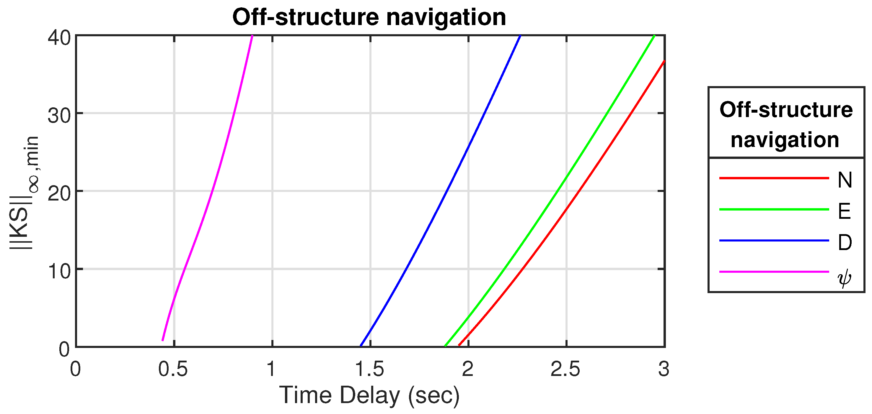
The results from the whole range of $\lambda$ can be seen in Figure 15 and Figure 16 for near-structure and off-structure navigation and chosen values are shown in

Table 10. Selected values for ${\parallel KS\parallel }_{\infty ,min}$.

$\mathit{\lambda }\left[\mathit{s}\right]$	0.00	0.60	1.20	1.80	2.40	3.00	3.60	4.20	4.80	5.40	6.00
Near-structure operation
N [$\mathrm{m}$]	-	4.11	11.98	19.02	25.77	-	-	-	-	-	-
E [$\mathrm{m}$]	-	4.80	11.36	17.01	22.36	27.65	-	-	-	-	-
D [$\mathrm{m}$]	-	9.28	24.18	37.65	50.72	-	-	-	-	-	-
$\psi$ [$\mathrm{rad}$]	-	34.41	-	-	-	-	-	-	-	-	-
Off-structure navigation
N [$\mathrm{m}$]	-	-	-	-	14.19	36.74	61.79	88.26	115.64	143.67	172.22
E [$\mathrm{m}$]	-	-	-	-	17.95	42.15	68.27	95.43	123.23	151.48	180.11
D [$\mathrm{m}$]	-	-	-	15.55	47.61	83.02	120.06	158.08	196.85	236.26	276.29
$\psi$ [$\mathrm{rad}$]	-	13.14	78.89	-	-	-	-	-	-	-	-

.

From Figure 15 and Figure 16 it can be seen that $\psi$ is much more affected by noise and output disturbances compared to the translational motions. Another observation is that off-structure navigation is more robust to noise than near-structure, which was expected as the scaling is smaller for near-structure operation. For some of the entries seen in Table 10 with small $\lambda$, there are no RHP poles, which is required in Equation (49); therefore, these has no value (-). In Table 10 it can also be seen that some not applicable values (-) appear when $\lambda$ gets sufficiently large, this is when the two conjugated complex poles turn into two real-valued poles.

5.3.3. Lower Bound for SG

As for ${\parallel KS\parallel }_{\infty ,min}$ there are no defined bounds for ${\parallel SG\parallel }_{\infty ,min}$ in regards to system controllability; however, as the transfer function describes the effects of input disturbances and pole uncertainties including uncertainty of time delays, due to Padé approximation, small values are preferred.

The results from the whole range of $\lambda$ can be seen in Figure 17 for near-structure and Figure 18 for off-structure navigation and chosen values for both cases are shown in

Table 11. Selected values for ${\parallel SG\parallel }_{\infty ,min}$.

$\mathit{\lambda }\left[\mathit{s}\right]$	0.00	0.60	1.20	1.80	2.40	3.00	3.60	4.20	4.80	5.40	6.00
Near-structure operation
N [$\mathrm{m}$]	-	0.12	0.85	2.50	5.26	9.22	14.46	21.03	28.94	38.23	48.90
E [$\mathrm{m}$]	-	0.12	0.81	2.31	4.74	8.16	12.61	18.10	24.65	32.28	40.98
D [$\mathrm{m}$]	-	0.07	0.42	1.20	2.45	4.21	6.49	9.30	12.65	16.54	20.98
$\psi$ [$\mathrm{rad}$]	-	1.39	10.22	31.80	69.95	127.42	206.30	308.16	434.24	585.50	762.71
Off-structure navigation
N [$\mathrm{m}$]	-	-	-	-	0.01	0.02	0.03	0.04	0.05	0.07	0.08
E [$\mathrm{m}$]	-	-	-	-	0.01	0.02	0.03	0.04	0.05	0.07	0.08
D [$\mathrm{m}$]	-	-	-	0.01	0.02	0.03	0.05	0.07	0.09	0.12	0.14
$\psi$ [$\mathrm{rad}$]	-	0.06	0.31	0.75	1.39	2.23	3.27	4.51	5.95	7.59	9.42

.

Both Figure 17 and Figure 18 shows that $\psi$ is highly affected by input disturbances and pole uncertainties compared to the translational motions. It can be noted that the discrete jumps, which are clearly seen in Figure 18 are present for both cases; however, it is not visible for the near-structure case due to the large magnitude for larger $\lambda$. Similar to the calculation of ${\parallel KS\parallel }_{\infty ,min}$, ${\parallel SG\parallel }_{\infty ,min}$ also requires an unstable system; therefore, no values are shown until the systems become unstable.

It can be seen that the tether is highly sensitive to disturbances compared to the transnational motions. Such disturbance could be the tether forces and torques acting on the ROV. The results of ${\parallel SG\parallel }_{\infty ,min}$ show that it would be beneficial to anchor the tether at COM to avoid the torque from the tether impacting the ROV [27].

6. Motion Sensor Evaluation

The results in previous sections allow for evaluating how the different time delays affect the control performance and ability to stabilize the system. However, the sensor technology used for pose measurement highly affects the size of the time delay. Therefore, the sensor’s usefulness is evaluated based on the results from the Input-Output controllability analysis.

In

Table 12. Typical motion sensor technologies and associated time delays.

Motion	Delay at LCL and UCL for ${\left|\right|\mathit{S}\left|\right|}_{\mathit{\infty },\mathbf{min}}$		Sensor Technology	Time Delay
	Near-Structure Operation	Off-Structure Navigation
N	LCL: 0.69 s	LCL: 3.44 s	LBL [19]	10 s [19]
	UCL: 1.22 s	UCL: 5.68 s	SBL [9,28]	1.50–2.50 s [9]
E	LCL: 0.66 s	LCL: 3.36 s	DVL [19,27,29]	0.03–0.20 s [19] **
	UCL: 1.24 s	UCL: 5.63 s	Visual SLAM [18,30]	0.10–0.20 s [18]
D	LCL: 0.66 s	LCL: 2.61 s	Pressure [31] ***	0.00 s *
	UCL: 1.21 s	UCL: 4.35 s
$\psi$	LCL: 0.30 s	LCL: 0.78 s	FOG [32]	0.00 s *
	UCL: 0.47 s	UCL: 1.2 s	MEMS Gyroscope [32]	0.00 s *
			Compass	0.00 s *

Note: All time delays marked with ^* do have a small delay, as signal transition and data processing always results in small delays; however, relative to the other sensors, the delay can be neglected. ^** For the DVL, the delay is impacted by the distance to the seabed, as sound waves have a limited propagation in water [19]. ^***The sensor technologies used for N and E directions can also be used for D. However, pressure transmitters are almost always applied as the primary sensor for D.

, different sensor technologies can be seen with typical time delays and for which motions they are used.

From Table 10, it can be seen that the SBL system is not appropriate to use for near-structure operation as the LCL is 0.66–0.69 s for N and E, while the time delay is between 1.5 and 2.5 s. The delay could be reduced by utilizing a delayed-state Kalman filter [8]; however, this requires knowledge of the delay, which is hard to determine due to the change of the speed-of-sound in water [19]. The delay imposed by the DVL is within the limit at which the nominal closed-loop system becomes unstable, which means that no controller reconfiguration is required. However, the DVL is subject to position drift due to the integration of errors in the velocity signal. The DVL sensor can, therefore, usually not be used as a stand-alone sensor for extended operation periods [17]. Visual-SLAM technologies use cameras with time delays in the same range as a present for the DVL. However, cameras require good visibility in order to track features which can be challenging in turbid conditions [33]. Sonar sensors can enhance the robustness of the feedback in turbidity water. However, the data is often not as detailed [16].

For off-structure navigation, the LCLs at 3.44 s and 3.36 s for N and E, respectively, are higher than any of the time delays for the sensor technologies mentioned in Table 12. However, it would require a reconfiguration of the existing controller in order to stabilize the system, as the system becomes unstable at 1.94 s and 1.87 s for N and E, respectively.

For D, it can be seen that the control limits, LCL and UCL, are lower than for N and E. However, the sensor delay in pressure transmitters is minimal; this is considered a minor problem compared to finding sensors for N and E. Another observation from Figure 15 and Figure 16 is that D-direction is more sensitive to noise than N and E. However, pressure transmitters are known to have a small signal-to-noise ratio, which is why this is not considered a problem. The influence of disturbances is also dependent on time delay and, therefore, minimal.

For $\psi$, the time delay at which the system reaches the control limits lies much lower than for the translational motions. However, as either compass, fiber-optic gyroscope (FOG), or microelectromechanical systems (MEMS) gyroscopes are commonly used for heading measurement, this is not a problem. Compasses work by measuring the Earth’s magnetic field. Therefore, compasses would not be a good choice when working in areas rich in steel objects or structures that disturb the sensor. In cases with magnetic disturbances, gyroscopes are often used instead, however, MEMS gyroscopes often has drifts of 60${}^{\circ }$/h [17]. To compensate for drift, a filter has to be added. However, this will result in a larger time delay. Alternatively, a more expensive gyroscope like a FOG can be used, which only has a drift of 0.0001${}^{\circ }$/h.

Both sensor noise and reliability have to be considered when choosing the sensors for navigation. As mentioned in Section 2 line-of-sight between transponder and receivers are required for for LBL and SBL, as well as bottom-lock is required for DVL [34]. For both types of acoustic sensors, the change in speed of sound, if this is not correctly dealt with, could result in inaccurate readings. The speed-of-sound in water is affected by water temperature, salinity, and pressure [10], which can change locally and therefore can be hard to calculate correctly for the entire path. Therefore, it is important to investigate how the vehicle reacts to noise and measurement dropouts when designing the feedback and control system.

7. Conclusions and Future Work

This study evaluates how different sizes of time delays impact the motion control of an ROV. The study focuses on a non-linear ROV model linearized for two different operation points based on near-structure and off-structure navigation.

As the analysis requires a rational transfer function, the time delays have been approximated using a first-order Páde approximation. Furthermore, a nominal inner-loop controller has been added. This controller has been developed in previous work [15] and implemented to get a nominal closed-loop system, which is designed without considering time delay. A stability analysis is made for four SISO systems, which are ${\mathit{\tau }}_1\to N$, ${\mathit{\tau }}_2\to E$, ${\mathit{\tau }}_3\to D$, and ${\mathit{\tau }}_6\to \psi$, to evaluate at which amount of time delay the closed-loop system becomes unstable. The results from the stability analysis have shown that the amount of delay tolerated for the closed-loop systems is very different for the different types of operation. For near-structure operation, all 4 DOFs are unstable at a time delay of 0.28 s or more, while all translational motions are stable up until 1.44 s for off-structure navigation. Common for both types of operation is that $\psi$ is the most difficult DOF to control when considering time delay. This is also confirmed in the IO Controllability analysis, which concludes that no controller can stabilize $\psi$ with a time delay above 0.47 s for near-structure operation and 1.2 s for off-structure navigation.

Another conclusion from the IO Controllability analysis showed that D is more sensitive to noise than N and E. However, as pressure transmitters are typically used as feedback for D, this is not considered a problem regarding sensors. The signal-to-noise ratio for pressure transmitters is usually small.

The IO Controllability also showed that the input disturbances greatly impact $\psi$. It would, therefore, be beneficial to try to minimize the input disturbance, which could, for example, be done by anchoring the tether in the COM.

The time delay limitations for each DOF are evaluated against specifications for commonly used sensors for underwater navigation. From this evaluation, it can be concluded that even though $\psi$ has the tightest range that can be controlled, it will not be of great concern. Most sensors used for $\psi$, such as compass and FOG, have delays smaller than needed. However, some limitations in sensor choice have been discovered for N and E. LBL can have time delays above 10 s. At the same time, the upper control limits for off-structure navigation are 5.68 s and 5.63 s for N and E, respectively.

In summary the following can be concluded about using IO Controllability analysis for UUVs:

• The IO Controllability is only applicable for linear systems; therefore, the non-linear system has to be linearized, resulting in inaccuracies of the results depending on the grade non-linearity. The drag contains non-linear terms, which depend on the velocity of the ROV. The linear model will differ from the non-linear model when the velocities differ from the operation points. Multiple operation points have been chosen to remedy large deviations depending on the type of operation.
• Time delays are infinite-dimensional systems, which have to be approximated into a proper transfer function. The approximation can be made by using the Padé approximation; however, this results in some inaccuracies. The approximation introduces inverse responses, larger delays introduce larger inverse responses, and therefore, the approximation is more accurate at low time delays.
• The IO Controllability benefits from being an open-loop analysis proving theoretical bound for the closed-loop system. This means that the system can be evaluated in terms of control performance while being controller agnostic. This is especially beneficial when choosing various sensor technologies for the feedback system. The analysis can then be used to find the maximum tolerated time delay, at which it will no longer be possible to control the UUV.
• The IO Controllability analysis also shows that input disturbances and pole uncertainties have a greater impact on the heading motion than on the linear motions.

The presented work has focused on a nominal ROV model. Further sensitivity of the results based on changing model and environmental parameters such as drag coefficients and added mass coefficients are needed for investigating the effect of time delay in a non-nominal environment. In future work, controllers will be designed and experimentally validated. The results from the IO Controllability analysis will be used as a benchmark for the control performance of the designed controllers. A further investigation on sensors limitations and faults regarding near-structure operation will also be made. As discussed in Section 6, the sensors which are useful for near-structure in N and E motion in terms of time delay are either drifting as seen for DVL or lacking in the sense of robustness as visual sensors due to example turbidity. Therefore, sensor fusion could be used to get reliable feedback, which meets both time delay and long-term accuracy requirements.

References

Mai, C.; Pedersen, S.; Hansen, L.; Jepsen, K.; Yang, Z. Modeling and Control of Industrial ROV’s for Semi-Autonomous Subsea Maintenance Services. IFAC PapersOnLine2017, 50, 13686–13691. [Google Scholar] [CrossRef]
Mai, C.; Pedersen, S.; Hansen, L.; Jepsen, K.L.; Yang, Z. Subsea infrastructure inspection: A review study. In Proceedings of the 2016 IEEE International Conference on Underwater System Technology: Theory and Applications (USYS), Penang, Malaysia, 13–14 December 2016; pp. 71–76. [Google Scholar] [CrossRef]
Huvenne, V.A.; Robert, K.; Marsh, L.; Lo Iacono, C.; Le Bas, T.; Wynn, R.B. ROVs and AUVs. In Submarine Geomorphology; Springer International Publishing: Cham, Switzerland, 2018; pp. 93–108. [Google Scholar] [CrossRef]
Cleveland, C.J. Section 6—Oil. In Handbook of Energy Volume II: Chronologies Top Ten Lists and Word Clouds; Elsevier: Amsterdam, The Netherlands, 2014. [Google Scholar] [CrossRef]
Pedersen, S.; Løhndorf, P.; Yang, Z. Challenges in Slug Modeling and Control for Offshore Oil and Gas Productions: A Review Study. Int. J. Multiph. Flow2017, 88, 270–284. [Google Scholar] [CrossRef]
Anderson, M. Nondestructive testing of offshore structures. NDT Int.1987, 20, 17–21. [Google Scholar] [CrossRef]
Riquer, F.W.; Gronemeyer, M.; Horn, J. Finding stability bounds for delayed systems with uncertain parameters. In Proceedings of the 2021 European Control Conference (ECC), Delft, The Netherlands, 29 June–2 July 2021. [Google Scholar]
Ribas, D.; Ridao, P.; Mallios, A.; Palomeras, N. Delayed state information filter for USBL-Aided AUV navigation. In Proceedings of the 2012 IEEE International Conference on Robotics and Automation, Saint Paul, MN, USA, 14–18 May 2012; pp. 4898–4903. [Google Scholar] [CrossRef]
Pedersen, S.; Liniger, J.; Sørensen, F.F.; Schmidt, K.; von Benzon, M.; Klemmensen, S.S. Stabilization of a ROV in Three-dimensional Space Using an Underwater Acoustic Positioning System. IFAC PapersOnLine2019, 52, 117–122. [Google Scholar] [CrossRef]
Bardakov, R.N.; Kistovich, A.V.; Chashechkin, Y.D. Calculation of the sound velocity in stratified seawater based on a set of fundamental equations. Oceanology2010, 50, 297–305. [Google Scholar] [CrossRef]
Chen, Y.; Jiang, N. Robust H∞ control of nonlinear time-varying delay systems with polytopic uncertainty. In Proceedings of the 2013 25th Chinese Control and Decision Conference (CCDC), Guiyang, China, 25–27 May 2013; pp. 3308–3313. [Google Scholar] [CrossRef]
Olgac, N.; Sipahi, R. An exact method for the stability analysis of time-delayed linear time-invariant (LTI) systems. IEEE Trans. Autom. Control.2002, 47, 793–797. [Google Scholar] [CrossRef]
Olgac, N.; Sipahi, R. An improved procedure in detecting the stability robustness of systems with uncertain delay. IEEE Trans. Autom. Control.2006, 51, 1164–1165. [Google Scholar] [CrossRef]
Skogestad, S.; Postlethwaite, I.; Wiley, J.; New, C.; Brisbane, Y. Toronto. In Analysis and Design, 2nd ed.; Wiley and Sons: Hoboken, NJ, USA, 2006. [Google Scholar]
Von Benzon, M.; Sørensen, F.; Liniger, J.; Pedersen, S.; Klemmensen, S.; Schmidt, K. Integral sliding mode control for a marine growth removing ROV with water jet disturbance. In Proceedings of the 2021 European Control Conference (ECC), Delft, The Netherlands, 29 June–2 July 2021; pp. 2265–2270. [Google Scholar] [CrossRef]
Liniger, J.; Jensen, A.L.; Pedersen, S.; Sørensen, H.; Mai, C. On the autonomous inspection and classification of marine growth on subsea structures. In Proceedings of 2022 OCEANS Conference & Exposition, Oceans 2022, Chennai, China, 21–24 February 2022. [Google Scholar]
Paull, L.; Saeedi, S.; Seto, M.; Li, H. AUV Navigation and Localization: A Review. IEEE J. Ocean. Eng.2014, 39, 131–149. [Google Scholar] [CrossRef]
Amarasinghe, C.; Ratnaweera, A.; Maitripala, S. Monocular Visual SLAM for Underwater Navigation in Turbid and Dynamic Environments. Am. J. Mech. Eng.2020, 8, 76–87. [Google Scholar] [CrossRef]
Kinsey, J.C.; Eustice, R.M.; Whitcomb, L.L. A Survey Of Underwater Vehicle Navigation: Recent Advances And New Challenges. IFAC Conf. Manoeuvering Control. Mar. Craft2006, 88, 1–12. [Google Scholar]
Vickery, K. Acoustic positioning systems. A practical overview of current systems. In Proceedings of the 1998 Workshop on Autonomous Underwater Vehicles (Cat. No.98CH36290), Cambridge, MA, USA, 21–21 August 1998; pp. 5–17. [Google Scholar] [CrossRef]
Fossen, T.I. Handbook of Marine Craft Hydrodynamics and Motion Control, 1st ed.; Wiley: Hoboken, NJ, USA, 2011. [Google Scholar]
Jepsen, K.L.; Hansen, L.; Yang, Z. Control parings of a de-oiling membrane process. IFAC PapersOnLine2018, 51, 126–131. [Google Scholar] [CrossRef]
Jepsen, K.L.; Pedersen, S.; Yang, Z. Control pairings of a deoiling membrane crossflow filtration process based on theoretical and experimental results. J. Process Control2019, 81, 98–111. [Google Scholar] [CrossRef]
Hanta, V.; Procházka, A. Rational approximation of time delay. Inst. Chem. Technol. Prague. Dep. Comput. Control Eng. Tech.2009, 5, 28. [Google Scholar]
Skogestad, S.; Grimholt, C. The SIMC method for smooth PID controller tuning. Adv. Ind. Control.2012, 147–175. [Google Scholar] [CrossRef]
Jahanshahi, E.; Skogestad, S.; Helgesen, A.H. Controllability analysis of severe slugging in well-pipeline-riser systems. IFAC Proc. Vol.2012, 45, 101–108. [Google Scholar] [CrossRef] [Green Version]
Karmozdi, A.; Hashemi, M.; Salarieh, H. Design and practical implementation of kinematic constraints in Inertial Navigation System-Doppler Velocity Log (INS-DVL)-based navigation. Navigation2018, 65, 629–642. [Google Scholar] [CrossRef]
Snyder, J. Doppler Velocity Log (DVL) navigation for observation-class ROVs. In Proceedings of the OCEANS 2010 MTS/IEEE SEATTLE, Seattle, WA, USA, 20–23 September 2010; pp. 1–9. [Google Scholar] [CrossRef]
Jian, M.; Liu, X.; Luo, H.; Lu, X.; Yu, H.; Dong, J. Underwater image processing and analysis: A review. Signal Process. Image Commun.2021, 91, 116088. [Google Scholar] [CrossRef]
Balavalad, K.B.; Sheeparamatti, B.G. A Critical Review of MEMS Capacitive Pressure Sensors. Sens. Transducers2015, 187, 120–128. [Google Scholar]
Passaro, V.M.N.; Cuccovillo, A.; Vaiani, L.; Carlo, M.D.; Campanella, C.E. Gyroscope Technology and Applications: A Review in the Industrial Perspective. Sensors2017, 17, 2284. [Google Scholar] [CrossRef] [PubMed] [Green Version]
O’Byrne, M.; Ghosh, B.; Pakrashi, V.; Schoefs, F. Effects of turbidity and lighting on the performance of an image processing based damage detection technique. Safety, reliability, risk and life-cycle performance of structures and infrastructures. In Proceedings of the 11th International Conference on Structural Safety and Reliability, ICOSSAR 2013, New York, NY, USA, 16–20 June 2013; pp. 2645–2650. [Google Scholar] [CrossRef]
Troni, G.; Whitcomb, L.L. Experimental evaluation of a MEMS inertial measurements unit for Doppler navigation of underwater vehicles. In Proceedings of the 2012 Oceans, Hampton Roads, VA, USA, 14–19 October 2012; pp. 1–7. [Google Scholar] [CrossRef]
Figure 1.
BlueROV2 with modification designed for cleaning operation.
Figure 2.
Cleaning mission example. The shaded green area is the operation area where a near-structure operation is performed.
Figure 3.
Photos of water jet nozzle used on BlueROV2. (a) Photo of the applied high-pressure water jet nozzle. (b) Photo of the BlueROV2 while the water jet is utilized.
Figure 4.
Test setup for cleaning test at Port of Esbjerg.
Figure 5.
BlueROV2 with frame-definitions.
Figure 6.
Comparison on flow simulation and experimental data for standard configuration BlueROV2.
Figure 7.
Drag force from flow simulation and corrected 2nd-order polynomial for drag.
Figure 8.
Analysis on the behavior of 1st order Padé approximation for .
Figure 9.
System diagram showing the nominal closed-loop system as state space and linear time-invariant system.
Figure 10.
Integrated absolute error for various time delays for near-structure operation.
Figure 11.
Integrated absolute error for various time delays for off-structure navigation.
Figure 12.
Block diagram showing the considered system including measurement noise (n).
Figure 13.
for Near-structure operation with upper and lower control bound.
Figure 14.
for off-structure navigation with upper and lower control bound.
Distance to Structure where is cleaning efficiency