Research on COD Soft Measurement Technology Based on Multi-Parameter Coupling Analysis Method

Abstract

This paper presents a soft measurement technique for COD (Chemical Oxygen Demand) based on the multiparameter coupling analysis method. First, through mechanism analysis and correlation analysis of historical data during the measurement process, water quality parameters, such as hydrogen potential (PH), dissolved oxygen (DO), turbidity (TU), and electrical conductivity (EC), can be used to estimate COD values. To further improve the estimation accuracy of the water quality parameter model, we adopted a modeling method combining a BP neural network and support vector machine, which showed an average relative error of 6.13% and an absolute coefficient of up to 0.9605. Finally, experiments in a lake environment demonstrate that this method shows excellent performance, with highly reliable and accurate prediction results.

1. Introduction

As water resources play an increasingly prominent role in global economic development and environmental protection [1,2], countries around the world are paying more attention to water environment protection issues, and have devoted enormous resources to support research on the monitoring and control of water environment pollution. The COD parameter is very important for showing the degree of water pollution [3,4,5,6]. In practice, COD sensors require frequent manual calibration, which prevents them from accurately measuring COD values for prolonged periods. To overcome this limitation, soft measurement technology has been proposed.

Soft measurement technology, also known as soft instrument technology, can undertake online real-time measurement tasks that are not possible with instrumentation or hardware detection and is widely used in many fields such as production process control, optimization and parameter monitoring [7,8,9,10]. With this approach, mechanism analysis or experimental data are used to select variables that can be easily and accurately measured as auxiliary variables, whereas those that cannot be directly and accurately measured are selected as dominant variables. After this selection process, a mapping relationship is constructed between them so that the prediction of process variables can be measured.

The existing chemical oxygen demand measurement methods cannot meet the needs of long-term outdoor water quality monitoring, and COD sensors also require frequent manual calibration and maintenance. In contrast, soft measurement technology has a host of advantages that makes it a more appealing alternative in practical situations. It is economical and reliable, has a rapid dynamic response, and replaces hardware with software. Because of these advantages, in this study, we propose a multi-parameter coupling analysis method based on COD measurement technology, which can achieve short-term estimation of the target parameter chemical oxygen demand and can enable the automatic underwater calibration of COD hardware sensors. Compared with existing measurement methods, this method is accurate and efficient, does not rely on hardware, and can provide a basis for the automatic underwater calibration of COD sensors. Moreover, it also effectively prolongs the manual calibration cycle, and greatly reduces monitoring costs.

2. Soft Measurement Method

2.1. Selection of Auxiliary Variables

The selection process of auxiliary variables includes three steps: primary selection of auxiliary variables, correlation analysis, and final determination of auxiliary variables. First, it is necessary to clarify the target of soft measurement, and to determine the dominant variable of chemical oxygen demand. On this basis, we have a deep understanding and familiarity with the measurement principles of soft sensor objects and related equipment, and can preliminarily determine the auxiliary variables that affect the dominant variables through mechanism analysis and literature investigation. The auxiliary variable selection range encompasses the variable parameters that can be collected accurately and in real time in the process of measurement. Then, the selected auxiliary parameters are screened and adjusted by correlation analysis.

The selection of auxiliary variables plays an important role in the establishment of the model, which not only affects the structure of the water quality parameter model, but also further affects the estimation accuracy of the model. There are more than 10 kinds of water quality parameters that characterize water quality, but they are not independent of one another. There are always strong or weak coupling relationships between multiple-parameters of water quality [11,12], and these relationships are enhanced in some specific scenarios.

Widespread studies have been conducted on the coupling relationships between multiple parameters of water quality [13,14,15,16], and certain achievements have been made. Through the mechanistic analysis of the measurement process and literature review, four water quality parameters—namely, pH turbidity (TU), dissolved oxygen (DO) and oxygen redox potential (ORP) were initially selected as auxiliary variables, all closely related to the content of organic matter in water. Biological activities such as the growth and respiration of organic matter can change the pH value of water bodies, and strong acidic and alkaline environment are not suitable for the survival of organic matter. The magnitude of turbidity is closely related to the concentration of organic pollutants in water. Dissolved oxygen is closely related to the presence of microorganisms in water, thus affecting the content of organic matter; if the dissolved oxygen is insufficient, it will have an impact on the physiological activities of microorganisms, while an excessively high concentration may also lead to excessive decomposition of organic pollutants, resulting in a lack of nutrients. Redox potential is a comprehensive reflection of redox reaction, and the change in ORP is directly related to the species of microorganisms and their respiration. In summary, the dominant variable of the water quality parameter model is COD, and the auxiliary variables are pH, TU, DO and ORP.

Correlation analysis is a statistical analysis method used to study the correlation between two or more random variables in the same status. At present, there are three kinds of correlation coefficients used to express the correlation between variables: Pearson’s correlation coefficient, Spearman’s correlation coefficient, and Kendall’s correlation coefficient. The correlation coefficient can be used to reflect the direction and degree of the changing trend between the two variables. Its value ranges from −1 to 1, with 0 indicating that the two variables are not related. Positive values indicate positive correlation, while negative values indicate negative correlation. The greater the absolute value of the correlation coefficient, the stronger the correlation.

Through the analysis of the historical monitoring data, the applicable conditions of Pearson’s correlation coefficient are satisfied, and the correlation analysis is performed using MATLAB software. Pearson’s correlation, also known as product difference correlation, was proposed by the British statistician Pearson in the 20th century [17]. It is a method used to calculate linear correlation. The equation for calculating Pearson’s correlation coefficient is shown in Equation (1):

$$\rho \left(X,Y\right)=\frac{\mathrm{cov}\left(X,Y\right)}{\sigma X\times \sigma Y}$$

(1)

where $\mathrm{cov}\left(X,Y\right)$ is the covariance of the variable (X, Y), and $\sigma X$ and $\sigma Y$ are their respective standard deviations.

Correlation analysis includes two parts: the correlation analysis between dominant variables and auxiliary variables and the correlation analysis between auxiliary parameter variables.

(1)

Study on the correlation between dominant variables and auxiliary variables:

In order to verify the correlation between COD and the four auxiliary variables, the historical monitoring data covering these parameters were selected for correlation analysis. Since there is no water quality monitoring project covering the selected five variables at the same time, the two water quality monitoring projects covering the most selected parameters were selected, in which the monitoring parameters of item 1 included COD, TU, DO, ORP and ammonia nitrogen (AN), while the monitoring parameters of item 2 included COD, pH, TU, DO and electrical conductivity (EC). The correlation coefficients are shown in

Table 1. Correlation coefficients of item 1.

	TU	DO	ORP	AN
COD	−0.270611	−0.815111	−0.376139	0.077064

and

Table 2. Correlation coefficients of item 2.

	pH	TU	DO	EC
COD	−0.368012	−0.712238	−0.715341	−0.830134

.

It can be seen from Table 1 and Table 2 that COD has a high correlation with the four auxiliary variables of primary selection. In addition, it also has a high correlation with EC, but a low correlation with AN.

(2)

Study on the correlation between auxiliary parameter variables:

In order to further adjust the auxiliary parameters of the water quality parameter model, the correlation between the selected auxiliary variables was also analyzed. If the correlation between the auxiliary variables is strong, it shows that there is duplicate information between the auxiliary variables, and the number of auxiliary variables can be reduced. Selecting the historical monitoring data of project 2, and carrying on the correlation analysis to the auxiliary variable parameters, we can obtain the correlation coefficients shown in

Table 3. Correlation coefficients between auxiliary variables.

	DO	ORP	TU
DO	1	0.809963	0.417029
ORP	0.809963	1	0.318108
TU	0.417029	0.318108	1

.

It can be seen from the table that the correlation between ORP and DO is very high, indicating that they contain a lot of repetitive information. At the same time, considering external factors such as economic conditions and the degree of difficulty of maintenance, the auxiliary variables of the water quality parameter model can be adjusted to pH, TU, DO and EC.

2.2. Data Conversion

To better elucidate the role of each water quality parameter in the soft sensor model, standardization of the raw data is necessary. This is because the auxiliary variable parameters all have different magnitudes and magnitude units, which can complicate the interpretation of the results since they are not measured on the same scale. Data standardization can mitigate the influence of different units and makes it possible to compare different water quality parameters [18]. In this article, we employ and improve on the min-max standardization technique by transforming the mapping interval to [−1, +1].

2.3. Implementation of the Water Quality Parameter Model

The establishment of a water quality parameter model is at the core of soft sensor technology. Specifically, the mapping relationship between auxiliary variables and dominant variables needs to be analyzed in order to build a soft measurement model for water quality parameters. The establishment and offline training of the water quality parameter model were implemented in MATLAB. The training steps of the water quality parameter model are as follows:

• Set chemical oxygen demand as the label, and eliminate the PH, TU, DO and EC data of the original samples to form the training set;
• Normalize the PH, TU, DO, and EC data;
• Train the normalized data and corresponding labels to obtain water quality parameter models.

3. Modeling Method

3.1. Water Quality Parameter Modeling Based on a BP Network

Considering the complexity and nonlinearity of water quality parameter measurement, this study adopts a water quality parameter model based on a 3-layer BP neural network. The basic components of this neural network include 1 input layer, 1 hidden layer and 1 output layer, with the input layer containing 4 neurons and the output layer containing 1 neuron [19,20,21]. The tansig function is selected as the transfer function from the input layer to the hidden layer, whereas the purelin function is selected as the transfer function from the hidden layer to the output layer. The mean square error (MSE) between the model output and the desired output is used as the evaluation index to determine whether the training requirements are met.

The original data used in this study were selected from the historical monitoring data of the wireless water quality monitoring project of Zhongtian Ocean Systems Co. from 0:00 on 10 June 2019 to 11:00 on 19 June 2019, with a total of 338 sets of valid data points. For the purposes of this study, the first 300 sets were selected for training the water quality parameter model, whereas the last 38 groups were used as the validation set for simulation analysis.

In order to determine the optimal number of neurons in the hidden layer and the optimal learning algorithm of the BP neural network model, neural network models with different structures were designed to help determine the training process parameters. According to the previous analysis of BP neural network learning algorithms, three different learning algorithms-gradient descent method (TrainGD), adaptive learning rate momentum gradient descent method (TrainGDX) and the Levenberg-Marquardt method (TrainLM) were selected. At the same time, the number of neurons in the hidden layer was adjusted continuously, and the maximum number of iterations (ep) of the training parameters of the model alone with the mean square error (MSE) of the sample data, were observed. The number of neurons in the different hidden layers and the corresponding iterative times and errors of the learning algorithms, are shown in

Table 4. The number of neurons in different hidden layers and the corresponding iterative times and errors of the learning algorithms.

	5		6		7		8
	ep	MSE	ep	MSE	ep	MSE	ep	MSE
TrainGD	1000	0.00828	1000	0.0129	1000	0.0115	1000	0.00537
TrainGDX	124	0.00876	127	0.00502	45	0.0314	167	0.00252
TrainLM	12	0.00116	17	0.000961	12	0.00302	10	0.000989
	9		10		11		12
	ep	MSE	ep	MSE	ep	MSE	ep	MSE
TrainGD	1000	0.00838	1000	0.0104	1000	0.0124	1000	0.0168
TrainGDX	173	0.00460	165	0.00411	162	0.00241	164	0.00341
TrainLM	8	0.000947	13	0.000994	4	0.000998	6	0.000954

.

It can be seen from Table 4 that the convergence speed of the gradient descent method is too slow to achieve the desired target error within the specified maximum number of iterations. Although the adaptive learning rate momentum gradient descent method can achieve the desired target error within the specified maximum number of iterations, compared with the Levenberg–Marquardt algorithm, the required number of iterations for training is increased and the training error is obviously greater, indicating that the LM learning algorithm is more suitable for this model. The number of neurons in the hidden layer of the model was set as 9, and Levenberg–Marquardt was selected as the learning algorithm. A schematic representation of the static water quality parameter model based on the BP neural network (SWQM) is presented in Figure 1.

The 300 sets of training data were proportionally divided into a training set (70%), validation set (15%) and test set (15%) for model training. As shown in the Figure 2, after 8 epochs, the mean squared error met the requirements and the model stopped training.

As shown in the Figure 3, the correlation coefficients between the output results of the training set, validation set and test set of the SWQM model and the expected output were 0.98449, 0.98061, and 0.98575, respectively. For the entire training example, the correlation coefficient between the output results and the expected output was 0.98382.

To increase the estimation accuracy of chemical oxygen demand and make full use of the limited data, we added the changes of in PH, TU, DO and EC as auxiliary variables based on the original auxiliary variables. For the dominant variable parameters, the BP neural network was selected as the modeling algorithm, and a dynamic water quality parameter model based on the BP neural network (DWQM) was further proposed. X2, X4, X6 and X8 are the D-values between the current dataset and the previous dataset. After the data have been normalized, the D-values can be directly input into the neural network model. It should be noted that in order to ensure the uniformity of the D-value, the training set data must be input into the neural network from the second group. A schematic representation of the model structure is shown in the following Figure 4.

The Figure 5 below show the offline training of the DWQM model. After 13 epochs, the mean square error of the model met the requirements, and the model stopped training.

As shown in Figure 6, the correlation coefficients between the output results of the training set, validation set and test set of the DWQM model and the expected output were 0.98598, 0.98769, and 0.98464, respectively. The output results of the entire training sample had a correlation coefficient of 0.98597 with the expected output.

The mean relative error (MRE) and the absolute coefficient $R^2$ were selected as the evaluation indicators for the estimation ability of the water quality parameter model. The equation for calculating the average relative error is as follows:

$$MRE=\frac{1}{m}{\displaystyle \sum _1^m\frac{\left|x_i-{\widehat{x}}_i\right|}{x_i}}$$

(2)

where $x_i$ is the measured value, ${\widehat{x}}_i$ is the estimated value, and m is the number of sample data.

The equation for calculating the coefficient of determination is as follows:

$$R^2=\frac{SSR}{SST}=1-\frac{SSE}{SST}$$

(3)

where SST = SSR + SSE, SST is the total sum of squares, SSR is the regression sum of squares, and SSE is the residual sum of squares. The smaller the MRE, the closer $R^2$ is to 1 and the better estimation accuracy of the model.

The last 38 groups of data were used to test the simulation and estimation accuracy of the model. The simulation results of the SWQM model are shown in Figure 7. The average relative error MRE = 9.45% and the absolute coefficient $R^2=0.8918$.

The simulation results of the DWQM model are shown in Figure 8. The average relative error MRE = 8.21% and the absolute coefficient $R^2=0.9110$.

It can be seen from the simulation results that both the SWQM model and the DWQM model can estimate the changing trend of chemical oxygen demand. Compared with the SWQM model, the DWQM model shows smaller average relative error (MRE) and a larger absolute coefficient, indicating that the improved model is more suitable for the numerical estimation of COD.

3.2. Water Quality Parameter Model Based on Combined Prediction

To further improve the estimation accuracy of the water quality parameter model, a combination of multiple modeling methods should be adopted. The water quality parameter model based on a BP neural network only considers the influence of other water quality parameters on chemical oxygen demand in the same time dimension, but ignores the influence of water quality parameters in the previous stage—such as chemical oxygen demand and other water quality parameters—on the current oxygen demand value. The analysis of the simulation results of the water quality parameter model based on the BP neural network shows that significant changes in the chemical oxygen demand value can increase the chemical oxygen demand estimation error, indicating that the water quality parameter model based on the BP neural network is relatively robust to fluctuations in the water quality state. The water COD value shows good estimation accuracy, but when there are great changes in the water environment, a single prediction model can no longer meet the estimation needs. Instead, a prediction method based on time-series analysis needs to be supplemented—with trend forecasting performed to revise the final COD estimate. A schematic diagram of the water quality parameter model based on combined prediction is shown in Figure 9.

Specifically, the water quality parameter model based on the BP neural network completes offline training using a large amount of historical monitoring data, and undertakes the main prediction task of the combined prediction model. Meanwhile, the water quality parameter model based on a support vector machine (SVM) is trained online in real time using the water quality data collected on the previous day to perform auxiliary correction on the prediction results. When the water quality changes significantly, greater weight is given to the estimated value of the water quality parameter model based on the SVM in the combined prediction model. The equation for calculating the chemical oxygen demand of the combined prediction model is as follows:

$$COD=\left(1-\alpha \right)\ast CO{D}_{BP}+\alpha \ast CO{D}_{SVM}$$

(4)

where $CO{D}_{BP}$ is the estimated value of the COD of the water quality parameter model based on the BP neural network, $CO{D}_{SVM}$ is the estimated value of the COD of the water quality parameter model based on the SVM, and $\alpha$ is the correction coefficient. According to the chemical oxygen demand of the water quality parameter model based on the BP neural network, the estimated value of oxygen demand and the measured value of chemical oxygen demand are adjusted in real time.

The offline training of the water quality parameter model based on combined prediction is shown in the Figure 10. After 24 epochs, the mean square error of the water quality parameter model based on combined prediction meets the requirements, and the model stops training.

As shown in the Figure 11, the correlation coefficients between the output results of the training set, validation set and test set of the CWQM model and the expected output are 0.99153, 0.99215, and 0.98915. For the entire training example, the correlation coefficient between the output results and the expected output is 0.99048.

As shown in the Figure 12, the simulation results of the water quality parameter model based on combined prediction indicate an average relative error (MRE) of 6.13% and an absolute coefficient of 0.9605. Compared with the two water quality parameter models based on the BP neural network, the average relative error (MRE) is further reduced, and the absolute coefficient $R^2$ is also improved.

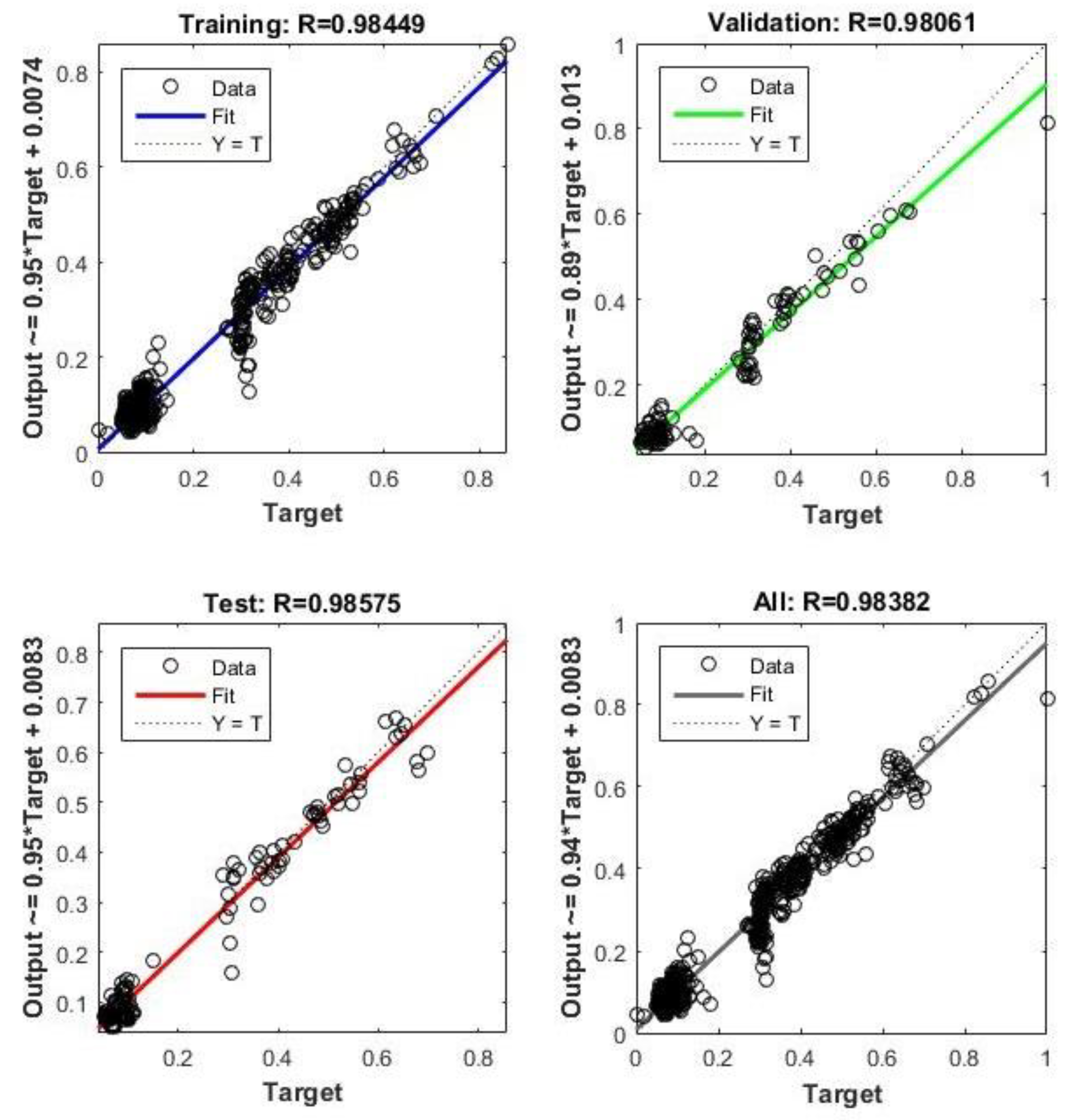
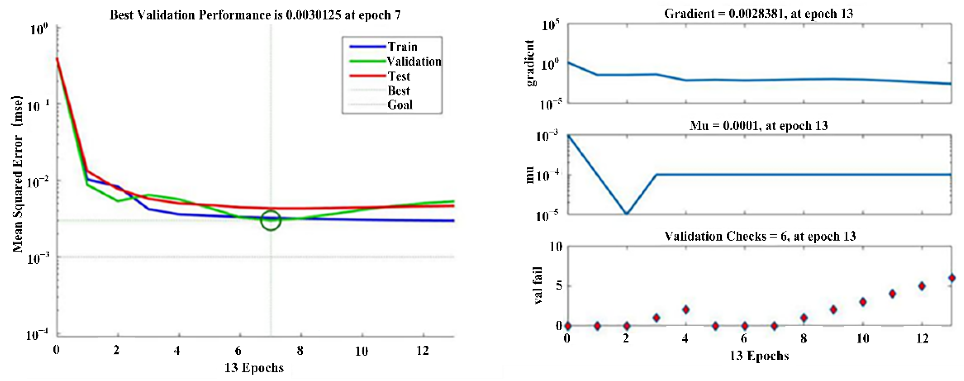
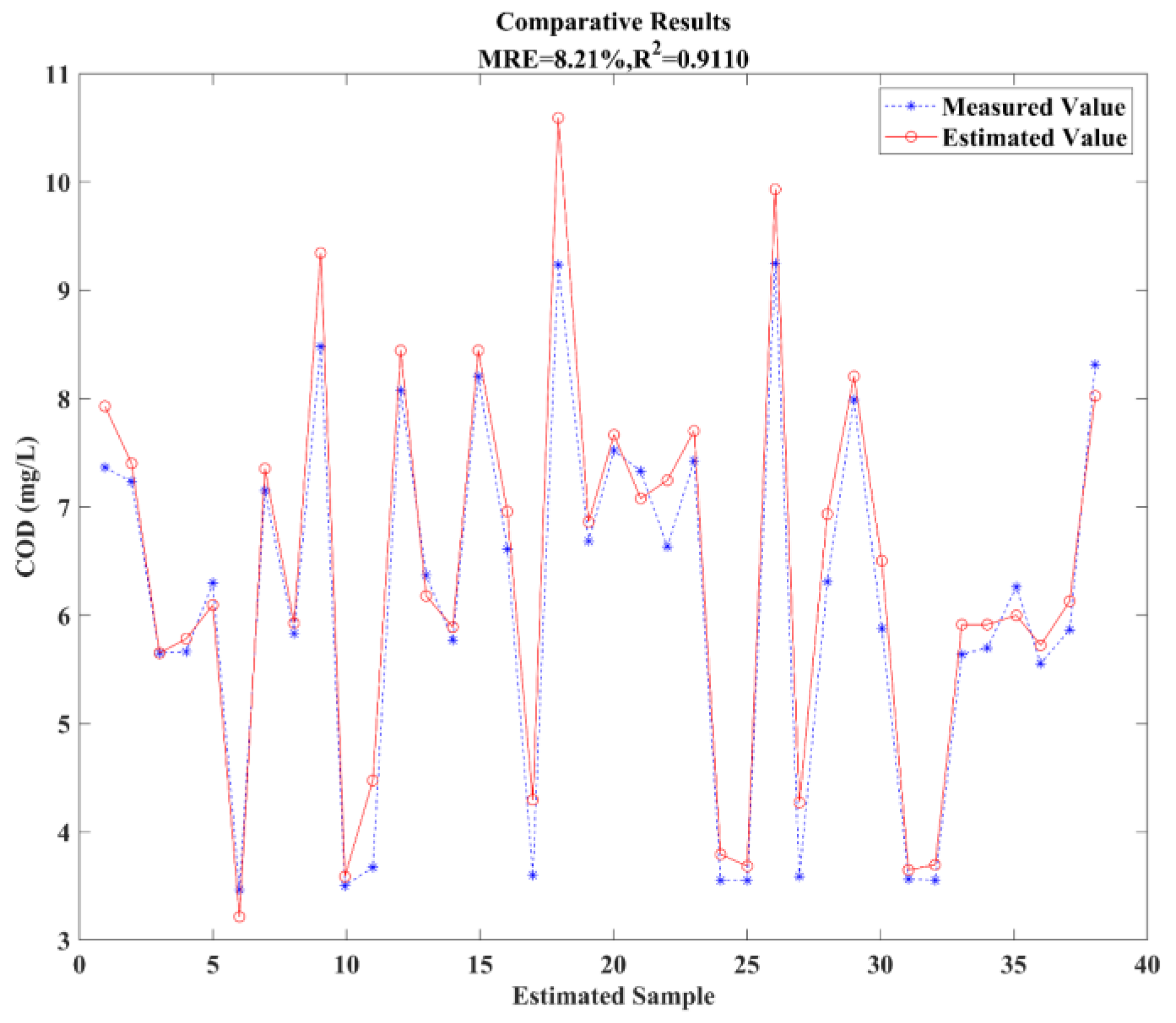
4. Experimental Validation

The hardware circuit of this paper was designed according to the experimental requirements and was divided into functional modules. The Figure 13 and Figure 14 show the hardware circuit architecture of the COD online estimation system, which is divided into five functional modules.

The machine monitoring interface runs on a remote client terminal and is the upper computer software program of the COD online estimation system. It is responsible for receiving the data uploaded by the lower computer, calling the water quality parameter model and carrying out the online estimation of COD values.

In July 2019, to verify the availability and stability of the COD measurement technology based on the multi-parameter coupled analysis method, we went to Yunhu, in the city of Nantong to conduct a one-week lake experiment using the COD online estimation system. The field test work is shown in Figure 15.

Through the pre-test experiment on the first day, it was found that under normal circumstances, there is little change in the water quality environment. To ensure a certain degree of volatility in the collected data, the measurement frequency of the system was set to 2 h, the test time was from 08:00 to 18:00 and continuous measurement was performed for 6 days. Altogether, a total of 36 sets of data were obtained. Then the measured values of the hardware sensor were compared with the estimated value of the system, and a line graph was drawn in Figure 16. The experimental results show that the COD online estimation system can accurately measure the trend of chemical oxygen demand in the target water environment and meets the design requirements of the system. Moreover, it provides a basis for the online calibration of portable COD sensors, prolongs the manual maintenance cycle, and effectively reduces the use cost.

The lake experiment results show that the COD online estimation system is reliable and stable, even during long service hours. The overall relative error of the 36 datasets was 6.97%, and the absolute coefficient was 0.9393, both of which indicate high estimation accuracy. Altogether, 33 groups of data fall within the relative error, with only 1 dataset exceeding the error range (i.e., data efficiency higher than 90%). Collectively, these results demonstrate that the online system is highly reliable.

5. Summary and Discussion

This paper proposes a COD measurement technology based on the multiparameter coupling analysis method and designs a COD online estimation system. The COD measurement technology based on the multi-parameter coupled analysis method proposed in this paper provides a low-cost, real-time method for the monitoring of chemical oxygen demand in natural water. It can be used with COD hardware sensors to extend the manual maintenance period and reduce the cost of use.

There are a number of advantages associated with the use of the water quality parameter model as the method of measurement of chemical oxygen demand, including strong environmental adaptability, a long maintenance period and low cost of use. Furthermore, the model is especially suitable for monitoring the needs of complex water environment and high labor maintenance costs, such as when the outdoor monitoring conditions are poor and the monitoring points are scattered. Compared with existing online water quality monitoring systems, the combination of the hardware sensors and control circuits of the monitoring nodes and the soft measurement modeling method is more tailored to such monitoring activities.

Despite such promising findings, some limitations of our study must be duly acknowledged. Due to limited sample data, the water quality parameter model can only be estimated accurately over a short period of time. Estimation errors increase when the time exceeds 1 month. Therefore, soft measurement cannot completely replace the hardware sensors but can only serve as an auxiliary measurement technique by prolonging the manual maintenance cycle of the hardware sensor, and reducing the cost of use. In future research, long term sample datasets should be collected. Based on changes in water quality, the datasets can be divided into multiple sub-sample datasets of different periods, and the modeled and estimated separately. Through more targeted sample data, the effective estimation period of the water quality parameter model can be extended, the maintenance period of the hardware sensor can be further extended, and the cost of use can be further reduced.

A second direction worth pursing in future research pertains to the generalizability of the system. If a soft measurement system is only developed for a specific measurement process and specific measurement conditions, the application of the system to other different working environments will be difficult, and will incur huge costs. In future research, multiple sample data on water quality parameters should be collected so that a basic estimation model of each water system can be established. In practical applications, only a small number of water quality parameter data of the target water body needs to be collected, and a similar basic estimation model can be further trained via techniques such as transfer learning to obtain the final estimation model. This can reduce repetitive modeling and improve system performance.

In addition, more attempts can be implemented on modeling methods, such as using emerging technologies for soft sensor modeling, or establishing soft sensor models with better performance. It is also a worthwhile pursuit to try to apply some of the latest research results to the modeling of soft sensors in order to further solve practical needs.

References

1. Maharjan, L.; Tripathee, L.; Kang, S.; Ambade, B.; Chen, P.; Zheng, H.; Li, Q.; Shrestha, K.; Sharma, C. Characteristics of Atmospheric Particle-bound Polycyclic Aromatic Compounds over the Himalayan Middle Hills: Implications for Sources and Health Risk Assessment. Asian J. Atmos. Environ. 2021, 15, 19. [Google Scholar] [CrossRef]
2. Ambade, B.; Sethi, S.S.; Chintalacheruvu, M.R. Distribution, risk assessment, and source apportionment of polycyclic aromatic hydrocarbons (PAHs) using positive matrix factorization (PMF) in urban soils of East India. In Environmental Geochemistry and Health; Springer: Berlin/Heidelberg, Germany, 2022. [Google Scholar] [CrossRef]
3. Zhu, S.; Han, H.; Guo, M.; Qiao, J. A data-derived soft-sensor method for monitoring effluent total phosphorus. Chin. J. Chem. Eng. 2017, 25, 1791–1797. [Google Scholar] [CrossRef]
4. Zare Abyaneh, H. Evaluation of multivariate linear regression and artificial neural networks in prediction of water quality parameters. J. Environ. Health Sci. Eng. 2014, 12, 40. [Google Scholar] [CrossRef] [PubMed] [Green Version]
5. Guoqiang, Y.; Weiguang, L.; Hao, W. Study of RBF Neural Network Based on PSO Algorithm in Nonlinear System Identification. In Proceedings of the 2015 8th International Conference on Intelligent Computation Technology and Automation (ICICTA), Nanchang, China, 14–15 June 2015; pp. 852–855. [Google Scholar]
6. Li, Y.; Shi, Y.; Wang, K.; Sun, D.; Yang, D. Design of online monitoring device for COD parameter in industrial sewage based on soft measurement method. In Proceedings of the 2017 32nd Youth Academic Annual Conference of Chinese Association of Automation (YAC), Hefei, China, 19–21 May 2017; pp. 959–964. [Google Scholar]
7. Cai, Y.; Fu, X.; Gao, X.; Li, L. Research progress of on-line automatic monitoring of chemical oxygen demand (COD) of water. IOP Conf. Ser. Earth Environ. Sci. 2018, 121, 022039. [Google Scholar] [CrossRef]
8. Hamed, M.M.; Khalafallah, M.G.; Hassanien, E.A. Prediction of wastewater treatment plant performance using artificial neural networks. Environ. Model. Softw. 2004, 19, 919–928. [Google Scholar] [CrossRef]
9. Mjalli, F.S.; Al-Asheh, S.; Alfadala, H.E. Use of artificial neural network black-box modeling for the prediction of wastewater treatment plants performance. J. Environ. Manag. 2007, 83, 329–338. [Google Scholar] [CrossRef] [PubMed]
10. Nair, A.; Hykkerud, A.; Ratnaweera, H. Estimating Phosphorus and COD Concentrations Using a Hybrid Soft Sensor: A Case Study in a Norwegian Municipal Wastewater Treatment Plant. Water 2022, 14, 332. [Google Scholar] [CrossRef]
11. Prada, J.; Dorronsoro, J.R. General noise support vector regression with non-constant uncertainty intervals for solar radiation prediction. J. Mod. Power Syst. Clean Energy 2018, 6, 268–280. [Google Scholar] [CrossRef] [Green Version]
12. Choi, Y.; Park, Y.; Hwang, J.; Jeong, K.; Kim, E. Improving Ocean Forecasting Using Deep Learning and Numerical Model Integration. J. Mar. Sci. Eng. 2022, 10, 450. [Google Scholar] [CrossRef]
13. Cinar, A.F.; Barhli, S.M.; Hollis, D.; Flansbjer, M.; Tomlinson, R.A.; Marrow, T.J.; Mostafavi, M. An autonomous surface discontinuity detection and quantification method by digital image correlation and phase congruency. Opt. Lasers Eng. 2017, 96, 94–106. [Google Scholar] [CrossRef]
14. Yan, W.; Tang, D.; Lin, Y. A Data-Driven Soft Sensor Modeling Method Based on Deep Learning and its Application. IEEE Trans. Ind. Electron. 2017, 64, 4237–4245. [Google Scholar] [CrossRef]
15. Najafzadeh, M.; Ghaemi, A. Prediction of the five-day biochemical oxygen demand and chemical oxygen demand in natural streams using machine learning methods. Environ. Monit. Assess. 2019, 191, 380. [Google Scholar] [CrossRef] [PubMed]
16. Kurwadkar, S.; Dane, J.; Kanel, S.R.; Nadagouda, M.N.; Cawdrey, R.W.; Ambade, B.; Struckhoff, G.C.; Wilki, R. Per- and polyfluoroalkyl substances in water and wastewater: A critical review of their global occurrence and distribution. Sci. Total Environ. 2022, 809, 151003. [Google Scholar] [CrossRef] [PubMed]
17. Benesty, J.; Chen, J.; Huang, Y.; Cohen, I. Pearson Correlation Coefficient. In Noise Reduction in Speech Processing; Springer: Berlin/Heidelberg, Germany, 2009; Volume 2, pp. 1–4, [Springer Topics in Signal Processing]; Available online: http://link.springer.com/10.1007/978-3-642-00296-0_5 (accessed on 9 May 2022).
18. Wang, G.; Jia, Q.S.; Zhou, M.; Bi, J.; Qiao, J.; Abusorrah, A. Artificial neural networks for water quality soft-sensing in wastewater treatment: A review. Artif. Intell. Rev. 2022, 55, 565–587. [Google Scholar] [CrossRef]
19. Li, X.; Liu, B.; Zheng, G.; Ren, Y.; Zhang, S.; Liu, Y.; Gao, L.; Liu, Y.; Zhang, B.; Wang, F. Deep-learning-based information mining from ocean remote-sensing imagery. Natl. Sci. Rev. 2020, 7, 1584–1605. [Google Scholar] [CrossRef]
20. Fan, L.; Boshnakov, K. Neural-network-based water quality monitoring for wastewater treatment processes. In Proceedings of the 2010 Sixth International Conference on Natural Computation, Yantai, China, 10–12 August 2010; pp. 1746–1748. [Google Scholar]
21. Aguado, D.; Ribes, J.; Montoya, T.; Ferrer, J.; Seco, A. A methodology for sequencing batch reactor identification with artificial neural networks: A case study. Comput. Chem. Eng. 2009, 33, 465–472. [Google Scholar] [CrossRef]
Figure 1. The SWQM model.
Jmse 10 00683 g001
Figure 2. Training error curve of the SWQM model.
Jmse 10 00683 g002
Figure 3. Correlation coefficient curves of the SWQM model.
Jmse 10 00683 g003
Figure 4. The DWQM model.
Jmse 10 00683 g004
Figure 5. Training error curve of the DWQM model.
Jmse 10 00683 g005
Figure 6. Correlation coefficient curves of the DWQM model.
Jmse 10 00683 g006
Figure 7. Comparative results of the SWQM model.
Jmse 10 00683 g007
Figure 8. Comparative results of the DWQM model.
Jmse 10 00683 g008
Figure 9. Water quality parameter model based on combination prediction (CWQM).
Jmse 10 00683 g009
Figure 10. Training error curve of the CWQM model.
Jmse 10 00683 g010
Figure 11. Correlation coefficient curves of the CWQM model.
Jmse 10 00683 g011
Figure 12. Comparative results of the water quality parameter model based on combined prediction.
Jmse 10 00683 g012
Figure 13. Hardware circuit architecture diagram of the COD online estimation system.
Jmse 10 00683 g013
Figure 14. pH/OD/EC/COD sensors.
Jmse 10 00683 g014
Figure 15. Lake experiment.
Jmse 10 00683 g015
Figure 16. Results of the lake experiment.
Jmse 10 00683 g016