Forecasting Shanghai Container Freight Index: A Deep-Learning-Based Model Experiment

Abstract

With the increasing availability of large datasets and improvements in prediction algorithms, machine-learning-based techniques, particularly deep learning algorithms, are becoming increasingly popular. However, deep-learning algorithms have not been widely applied to predict container freight rates. In this paper, we compare a long short-term memory (LSTM) method and a seasonal autoregressive integrated moving average (SARIMA) method for forecasting the comprehensive and route-based Shanghai Containerized Freight Index (SCFI). The research findings indicate that the LSTM deep learning models outperformed SARIMA models in most of the datasets. For South America and the east coast of the U.S. routes, LSTM could reduce forecasting errors by as much as 85% compared to SARIMA. The SARIMA models performed better than LSTM in predicting freight movements on the west and east Japan routes. The study contributes to the literature in four ways. First, it presents insights for improving forecasting accuracy. Second, it helps relevant parties understand the trends of container freight markets for wiser decision-making. Third, it helps relevant stakeholders understand overall container shipping market trends. Lastly, it can help hedge against the volatility of freight rates.

1. Introduction

Robust market forecasting is a critical and practical requirement in the management of shipping companies [1]. Prominent stakeholders in maritime business, such as carriers, freight forwarders, and shippers, rely on container freight-rate forecasts for operational decision making. Accordingly, various organizations continue to conduct periodic studies [2,3] on forecasting, and numerous researchers have actively studied improved prediction models.

Building reliable and robust forecasting models is essential in predicting market behavior and movements. Several techniques have been developed to build models that can estimate and forecast future time points, which can aid calculated decision-making to reduce risk and increase returns. The time-series forecasting method is becoming increasingly popular in various industries, including shipping.

In this study, we analyzed methods for predicting the Shanghai Containerized Freight Index (SCFI), which was chosen as the research object for three reasons. First, it has been studied in detail because it is one of the few container shipping freight indices that covers most of the global container trade volumes. It targets spot freight markets, which reflect up-to-date market trends and market equilibrium, and it provides high-frequency time-series data forecasts that reflect fluctuations in spot freight rates in Shanghai’s export container transport market. To calculate the SCFI, the Shanghai Shipping Exchange collects spot freight cost, together with insurance and freight (CIF) rates from the export container market, based on 13 shipping routes departing from the port of Shanghai on a container-yard-to-container-yard basis. The focus of this research, therefore, was the comprehensive SCFI, which is the weighted average of the 13 shipping routes.

Second, the SCFI is an underlying asset in freight derivatives [4]. In addition, time-series data forecasting, such as that provided by the SCFI, is highly important for business managers because these data reflect the overall trends in the corresponding container shipping market and provide implications for its future state.

Third, to date, the application of models for forecasting container freight rates has been relatively limited. Due to the high complexity, irregularity, randomness, and nonlinearity of time-series data, conventional econometric models cannot achieve a satisfactory forecasting accuracy.

Overall, few studies have been conducted on forecasting container freight rates by applying deep-learning algorithms. The goal of this study was to propose a novel LSTM-based forecasting model. The results of our evaluations complement the existing literature and indicate the need to develop more efficient forecasting techniques.

Our study resulted in three primary contributions. First, its findings can provide insights on improving forecasting accuracy. Second, the results of the study can aid in the understanding of freight trend forecasting in the corresponding container shipping market and enhance decision-making rationality in the shipping sector. Finally, the study provides implications for future investment in forward freight agreements or other risk-hedging freight derivatives.

The remainder of this paper is organized as follows: In Section 2, we review the literature on forecasting approaches in the shipping sector. Section 3, Section 4 and Section 5 present the properties of the associated data and describe the selected forecasting methods. In Section 6, we present our experimental results, including an assessment of forecasting accuracy in a given context. Finally, Section 7 presents discussions on our key findings and highlights the relevance of our work for practice and future research.

2. Literature Review

Forecasting shipping markets, particularly container freight-rate movements, has always been challenging. Over the past two decades, the global container shipping market has experienced turbulence due to several historical events. The first such event was the destruction of the shipping conference system in 2008 for port calls across all trades in the European Union (EU), marking the end of the cartel of shipping companies comprising the liner conference system [5]. The second was the global financial crisis of 2007–2008, which caused the container shipping freight market to significantly fluctuate along a generally downward-trending trajectory [2]. The third was the development of an unstable market environment characterized by the mergers and acquisitions of shipping lines, reformations of shipping alliances, and the commissioning of large container ships during the past decade, all of which contributed to heavy fluctuations in freight rates [6,7]. Recently, in the wake of the COVID-19 pandemic and the Suez Canal blockage, container shipping markets have become more unpredictable.

The methodologies applied in modeling container shipping include conventional econometric models, artificial intelligence (AI) models, or combinations of both, often referred to as hybrid models. Examples of research on econometric models include that of Chou et al. [8], in which a vector autoregression (VAR) model was used to forecast container trade volumes to Taiwan; Xie et al. [9] used autoregressive integrated moving average (ARIMA), SARIMA, and least-squares support vector regression (LSSVR) models to forecast container port throughputs; Schulze and Prinz [10], who reported that SARIMA models produced better results; and Kawasaki and Matsuda [11,12], who assessed the applicability of SARIMA and VAR models in forecasting container trade volumes.

Examples of AI model research include that of Chen and Chen [13], in which a genetic programming (GP) model was shown to outperform an ARIMA model by approximately 30%. An example hybrid model study is that of Xiao et al. [14], in which a transfer forecasting model guided by a discrete particle swarm optimization (TF-DPSO) algorithm was shown to outperform several existing models in terms of forecasting performance.

In recent years, other examples of hybrid models have emerged. Huang et al. [15] proposed a combination of projection pursuit regression (PPR) and GP algorithms. Xie et al. [16] proposed several hybrid approaches based on the LSSVR model and reported that their hybrid models achieved better forecasting performance than preprocessing methods such as SARIMA. Mo et al. [17] developed a hybrid model that applied SARIMA to the linear part of the data and support vector regression (SVR), back-propagation (BP), and GP to the nonlinear part; their research results indicated that the performance of the hybrid model was better than the other evaluated models.

Many approaches focus on forecasting container trade volumes and/or port throughput, but there are relatively few methods for forecasting container freight rates, especially the SCFI. Stopford [1] and Luo et al. [18] were pioneers in forecasting container freight rates by using supply and demand factors. Koyuncu and Tavacıoğlu [19] compared SARIMA and Holt–Winters Methods in forecasting the SCFI, and they concluded that the SARIMA model provided comparatively better results than the existing freight-rate forecasting models while performing short-term monthly forecasts. Chen et al. [20] applied a decomposition–ensemble method that combines empirical mode decomposition (EMD) and the grey wave forecasting model to forecast the China Container Freight Index (CCFI), and they found that the proposed method performed better than random walk and autoregressive moving average model (ARMA) in multi-step-ahead prediction. Munim and Schramm [2] recently deployed an autoregressive conditional heteroscedasticity (ARIMARCH) model to forecast container freight rates in Asia–North Europe routes. They observed that the ARIMARCH model provided better results than existing freight-rate forecasting models while enabling short-term forecasts on weekly and monthly bases. In his most recent research, Munim [21] reported that a state-space Trigonometric seasonality, Box–Cox transformation, ARMA errors, Trend and Seasonal components (TBATS) model outperformed seasonal neural network autoregression (SNNAR) and SARIMA models.

Like real-world time-series data, a container freight index features high complexity, irregularity, randomness, and nonlinearity. It is often difficult for conventional methods such as ARIMA to achieve a high prediction accuracy. As a result, models based on artificial neural networks (ANNs) are gaining increasing attention because of their ability to effectively manage the nonlinearity of time-series data [22]. In addition, machine learning methods can be used to build nonlinear prediction models using large quantities of historical time-series data, making it possible to obtain prediction results that are more accurate than those of conventional statistical models through repeated and iterative training and learning to approximate real models.

The machine learning (ML) methods that have been applied include SVR and ANN. These methods have strong nonlinear function approximation abilities and can be applied to tree-based ensemble learning [23]. Hassan et al. [24] proposed a new approach based on typical time-series and ML to forecast freight demand in the US market. Their model self-enhances through a reinforcement learning framework applied over a rolling horizon. Barua et al. [25] thoroughly reviewed ML models applied in international freight transportation management (IFTM), stating that ML is a powerful tool that enables better prediction and more robust support in IFTM.

A review of the existing literature that focuses on applied methodologies is summarized in

Table 1. Literature review summary of forecasting techniques in the shipping sector.

Reference	Application	Method	Findings
Chou et al. [8]	Container trade volumes	VAR	A modified regression model for forecasting Taiwan’s inbound container volumes was proposed.
Kawasaki and Matsuda [11]	Container trade volumes	SARIMA	The residual had no autocorrelation, and the defined model could reproduce volumes of container movement with high accuracy.
Kawasaki and Matsuda [12]	Container trade volumes	VAR	The VAR model clarified the length of time that U.S. economic indicators affect the container trade movement from East Asia to the U.S.
Chen and Chen [13]	Container port throughput	Decomposition approach, SARIMA, GP	The GP model predictions were approximately 32–36% better than the decomposition approach and SARIMA.
Huang et al. [15]	Container port throughput	PPR with GP, ANN, SARIMA, and PPR	The proposed PPR-with-GP method significantly outperformed ANN, SARIMA, and PPR models.
Mo et al. [17]	Container port throughput	SARIMA, SVR, BP, and GP	A hybrid model was developed by applying SARIMA for the linear part and SVR, BP, and GP for the nonlinear part of the data. Results showed that the hybrid model performed better than others.
Xiao et al. [14]	Container port throughput	TF-DPSO, ARIMA, and Elman Neural network (ENN)	The forecasting performance of TF-DPSO was better than that of several existing models.
Xie et al. [16]	Container port throughput	LSSVR and OLS	The proposed hybrid LSSVR approach achieved better forecasting performance than OLS.
Xie et al. [9]	Container port throughputs	ARIMA, SARIMA, and LSSVR	Data characteristic analysis results suggest that hybrid models can perform better than other methods.
Schulze and Prinz [10]	Container port throughput and trade volumes	SARIMA and exponential smoothing approach	The SARIMA approach yielded slightly better-modeled values of container throughput than the exponential smoothing approach.
Luo et al. [18]	Container freight	Three-stage Least Squared (3SLS)	The overall model could explain more than 90% of the fleet capacity and freight-rate variations.
Munim and Schramm [2]	Container freight—FE–FE route of SCFI	ARIMARCH	The ARIMARCH model provided better results than the existing freight-rate forecasting models.
Munim and Schramm [23]	Container freight—SCFI, 4 routes	ARIMA, VAR, ANN, and SVR	Overall, VAR/VEC models outperformed ARIMA and ANN in training-sample forecasts.
Al Haji Hassan et al. [24]	Freight demand in the U.S.	time-series models with reinforcement learning framework	A new approach building on typical time-series and machine learning models to forecast the freight demand in the U.S. market was proposed.
Ubaid et al. [26]	Container freight, Asia/Oceania route	SVR, RFR, and GBR	The GBR model outperformed other models, with a test accuracy of 84%.
Chen et al. [20]	Container freight—CCFI	Decomposition–ensemble method based on EMD and grey wave forecasting model	The proposed method performed better than random walk and ARMA in multi-step-ahead prediction.
Koyuncu and Tavacıoğlu [19]	Container freight—SCFI	SARIMA and Holt–Winters Methods	The SARIMA model provided better results than the existing freight-rate forecasting models while performing short-term forecasts on a monthly rate.
Munim [21]	Container freight—CCFI	SARIMA, SNNAR, and the state-space TBATS model	The TBATS model or a combination of TBATS and SARIMA forecasts outperformed SARIMA and SNNAR, as well as their combinations.

Source: Author-compiled (models in bold letters indicate machine-learning-based models).

. To the best of our knowledge, the LSTM model has not been previously applied in container shipping-related research.

This study was intended to contribute to the existing literature by filling these research gaps. We propose a deep-learning-based LSTM model for forecasting SCFI time-series data.

3. Deep Learning

Deep learning is a subfield of machine learning techniques concerned with ANNs. The most popular deep learning algorithms include convolutional neural networks (CNNs), recurrent neural networks (RNN), and stacked auto-encoders (SAE), among others. LSTM is an RNN architecture that can process a sequence of inputs. Since its introduction by Hochreiter and Schmidhuber [27], it has been refined by many researchers.

3.1. Model Description

As a special type of RNN, LSTM processes the input in a sequential manner by computing the output from the input of the previous step. However, typical RNNs suffer from vanishing (and exploding) gradients arising from the repeated use of recurrent weight matrices. As they are calculated using the chain rule, RNN gradients must undergo continuous matrix multiplications during the backpropagation process, which causes the gradients to either exponentially shrink (vanish) or exponentially blow up (explode). LSTM does not suffer from this problem because its models introduce gating functions to prevent gradient vanishing.

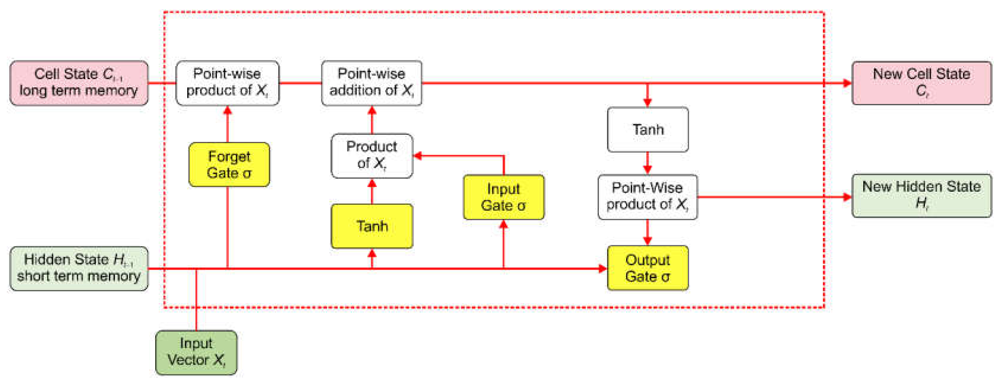
The LSTM is illustrated in Figure 1. It comprises a cell, input gate, output gate, and forget gate. The three gates regulate the flow of information into and out of the cell, and the cell remembers the values over any time interval. The gating functions enable the network to determine the extent to which the gradient vanishes and to obtain values at each time step. In other words, LSTM can process time-series data as a unit and can store, discard (forget), or add important information for making predictions, thus making it suitable for the analysis of time-series data.

3.1.1. Forget Gate (F)

The first step in LSTM is to identify the information to be discarded. The forget gate determines which information from the long-term memory is not required and should be discarded. This is performed by multiplying the incoming long-term memory with a forget vector generated by the current input and the incoming short-term memory:

$$F_t=\sigma (X_t{W}_x^F+C_{t-1}{W}_h^F+B^F)$$

(1)

where $X_t$ is the current input vector, $C_{t-1}$ is the output from the previous time step, $W_h^F$ is the weight, and $B^F$ is the bias in the forget gate layer.

3.1.2. Input Gate (I)

The second step in LSTM is the input gate that determines whether the new information is to be stored in the long-term memory. It works with information based on current input and short-term memory from the previous time step. The input gate is defined as follows:

$$I_t=\sigma (X_t{W}_x^I+C_{t-1}{W}_h^I+B^I)$$

(2)

where $X_t$ is the input vector, $C_{t-1}$ is the output from the previous time step, $W_h^I$ is the weight, and $B^I$ is the bias at the input gate layer.

3.1.3. Output Gate (O)

The output gate computes the current input, previous short-term memory, and newly-computed long-term memory to produce a new short-term memory or hidden state to be passed on to the cell in the next time step:

$$O_t=\sigma (X_t{W}_x^O+C_{t-1}{W}_h^O+B^O)$$

(3)

where $X_t$ is the input vector, $C_{t-1}$ is the output from the previous time step, $W_h^O$ is the weight, and $B^O$ is the bias in the output gate layer.

3.1.4. Activating Function

A hyperbolic tangent function (tanh) was used as the activating function in the proposed model. The tensor G applied to the input gate is expressed as follows:

$$G_t=tanh(X_t{W}_x^G+C_{t-1}{W}_h^G+B^G)$$

(4)

The new cell that stores long-term memory $C_t$ is then given by:

$$C_t=G_t\otimes I_t+F_t\otimes C_{t-1}$$

(5)

where ⊗ is the point-wise product.

The short- and long-term memories produced by the three gates are carried over to the next cell, and the neural network functions by repeating this process. The output of each time step obtained from the short-term memory is also called the hidden state, whose layer H is defined as:

$$H_t=O_t\otimes tanh{C}_t$$

(6)

where ⊗ is the point-wise product.

Unlike standard neural networks, LSTM has feedback connections, which enable it to remember values from earlier stages for future use. This ability to store information over a period of time is useful for managing time-series data.

LSTM has been applied to not only the processing of single data points for uses such as image captioning and generation but also the processing of entire data sequences for machine translation.

4. Data

Data Description

The dataset used in this study contained time-series data extracted from the composite SCFI from its inception in 2009 to April 2020. The total sample size was 548 for each data series, with 7672 data points (

Table 2. Description of data.

Index	Count	Mean	Standard Deviation	Minimum	25%	50%	75%	Maximum
SCFI (comprehensive index	548	994	324	400	795	951	1117	2885
NCMP (North Europe)	548	1027	513	205	738	907	1218	4452
MED (Mediterranean)	548	1070	508	195	761	944	1262	4298
USEC (U.S. East Coast)	548	1873	630	725	1457	1774	2115	4080
USWC (U.S. West Coast)	548	3068	744	1448	2563	3099	3455	5049
Persian (Persian Gulf and Red Sea)	548	739	298	211	530	711	902	1995
ANZ (Australia/New Zealand)	548	798	378	249	542	760	958	2490
WAF (East/West Africa)	548	2023	697	841	1624	1943	2323	6630
SAF (South Africa)	548	949	381	307	748	869	1081	3307
SAM (South America)	548	1713	1081	99	1097	1609	2119	8907
JPNW (West Japan)	548	253	75	77	215	231	332	382
JPNE (East Japan)	548	259	70	66	214	238	333	389
SEA (Southeast Asia)	548	204	119	53	145	185	235	974
KOR (Korea)	548	162	37	86	125	162	191	234

). The time granularity of the data was one week.

First, a stationarity check of dataset was conducted using the Dickey–Fuller (DF) test. Time-series data are said to be stationary if their statistical properties, such as the mean and variance, remain constant over time. In DF testing, the null hypothesis is that the time series is non-stationary, and the test results comprise a test statistic and some critical values relating to the different confidence levels. If the test statistic is less than the critical value, the null hypothesis can be rejected and the series can be considered stationary.

In this study, we chose to apply an augmented version of the DF test that is often applied to larger and more complicated sets of time-series models. The augmented DF (ADF) statistic we used is a negative number that firmly rejects the hypothesis that there is a unit root at some level of confidence as it becomes smaller. For a stationary series, the p-value (0 ≤ p ≤ 1) should be as low as possible and the critical values at different confidence intervals should be close to the test statistic value.

Prior to the treatment, the ADF test statistic was less than 5% of the critical value (

Table 3. Results of DF test for SCFI.

	Before Treatment	After Treatment
Test Statistic	−0.1205	−4.6303
p-value	0.9474	−0.0001
Number of Lags Used	12	17
Number of Observations Used	550	544

); therefore, the stationarity of the time series was rejected with 95% confidence.

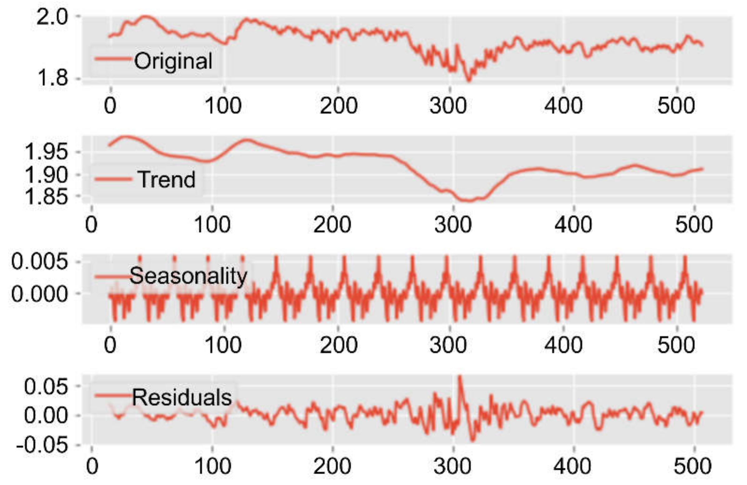
We conducted differencing, seasonal, and trend decomposition treatments using locally estimated scatterplot smoothing (LOESS STL) [28] to decompose trends and seasonality (Figure 2).

After treatment, the ADF test statistic was significantly lower than the 1% critical value (Table 3), indicating that the adjusted time series was close to stationary.

For the implementation, the dataset was split into training and testing sets. Cross-validation was performed with a time step of three for the training dataset (equaling 76% of the total dataset size). The testing dataset (24% of the total dataset size) was used to evaluate the performance of the models outside the training set while avoiding overfitting.

5. Methods

For comparison, we built a SARIMA model and a LSTM model.

5.1. SARIMA Model

The SARIMA model is one of the most important and widely used time-series models. The ARIMA model is the most general class of models for time-series forecasting because it can represent several different types of time series, that is, pure autoregressive (AR, often denoted as $p$), pure moving average (MA, often denoted as $q$), and integrated versions of stationary series (I, often denoted as $d$). ARIMA accepts data that are either non-seasonal or have the seasonal component removed, e.g., data that are seasonally adjusted via methods such as seasonal differencing. A non-seasonal ARIMA model can be classified as $ARIMA\left(p,d,q\right)$, where:

$p$: trend autoregressive order.

$d$: trend difference order (the number of non-seasonal differences needed for stationarity).

$q$: trend moving average order (the number of lagged forecast errors in the prediction equation).

The general form of the $ARMA\left(p,q\right)$ equation for forecasting time series $y$ is given as:

$$y_t=c+{\theta }_1{y}_{t-1}+{\theta }_2{y}_{t-2}+\dots +{\theta }_p{y}_{t-p}+{\epsilon }_t-{\phi }_1{\epsilon }_{t-1}-{\phi }_2{\epsilon }_{t-2}-\dots -{\phi }_q{\epsilon }_{t-q}$$

(7)

where $c$ is a constant; $y_t$ and ${\epsilon }_t$ are the actual value and random error at time period $t$, respectively; and ${\theta }_i\left(i=1,\dots ,p\right)$ and ${\phi }_j\left(j=0,\dots ,q\right)$ are the AR and MA parameters, respectively. The error terms ${\epsilon }_t$ are assumed to be independently and evenly distributed, with a mean of zero and a constant variance of ${\sigma }^2$. If $q=0$, then Equation (7) becomes an AR model of order $p$; if $p=0$, the model reduces to an MA model of order $q$. To consider the integration (I) part, $d$ is defined in terms of $y$, the n^th difference of $Y$, as follows:

If $d=0$: $y_t=Y_t$;

If $d=$1: $y_t=Y_{t-1}$;

If $d=2$: $y_t=(Y_t-Y_{t-1})-\left(Y_{t-1}-Y_{t-2}\right)={\mathrm{Y}}_{\mathrm{t}}-2Y_{t-1}+Y_{t-2}$.

Frequent seasonal effects come into play in many time-series datasets, especially in the case of SCFI data because of the seasonal demand of container freight. In response, an SARIMA model can be formulated by including additional seasonal terms in the ARIMA model [29]. As an ARIMA model does not support seasonal data that reflect repeating cycles within a time series, we implemented an SARIMA model to reflect the clear seasonality of the SCFI (e.g., [30]), The seasonal part of the model comprised terms that are very similar to the non-seasonal components but include the backshifts of the seasonal period. In addition to the three hyperparameters $p$, $d,$ and $q$ in the ARIMA model, four seasonal elements $\left(P,D,Q,S\right)$ were configured as follows:

$P$: seasonal autoregressive order

$D$: seasonal difference order.

$Q$: seasonal moving average order

$S$: number of time steps for a single seasonal period.

The general form of the SARIMA model is denoted as $ARIMA\left(p,d,q\right)$ $\left(P,D,Q\right)s$, where $p$ is the non-seasonal AR order, $\mathrm{d}$ is the non-seasonal differencing, $q$ is the non-seasonal MA order, $P$ is the seasonal AR order, $D$ is the seasonal differencing, $Q$ is the seasonal MA order, and $s$ is the time span of the repeating seasonal pattern. The SARIMA model can be written as follows:

$$y_t=c+{\displaystyle \sum }_{i=1}^p{\theta }_1{y}_{t-1}+{\displaystyle \sum }_{i=1}^P{\Theta }_i{y}_{t-is}+{\epsilon }_t-{\displaystyle \sum }_{j=1}^q{\phi }_j{\epsilon }_{t-j}-{\displaystyle \sum }_{j=1}^Q{\Phi }_j{\epsilon }_{t-js}$$

(8)

where $p$, $q$, $P$, $Q$, ${\theta }_i$, and ${\phi }_j$ are as defined previously and ${\Theta }_i \left(i=1, \dots , is\right)$ and ${\Phi }_j\left(j=1, \dots , js\right)$ are their seasonal counterparts.

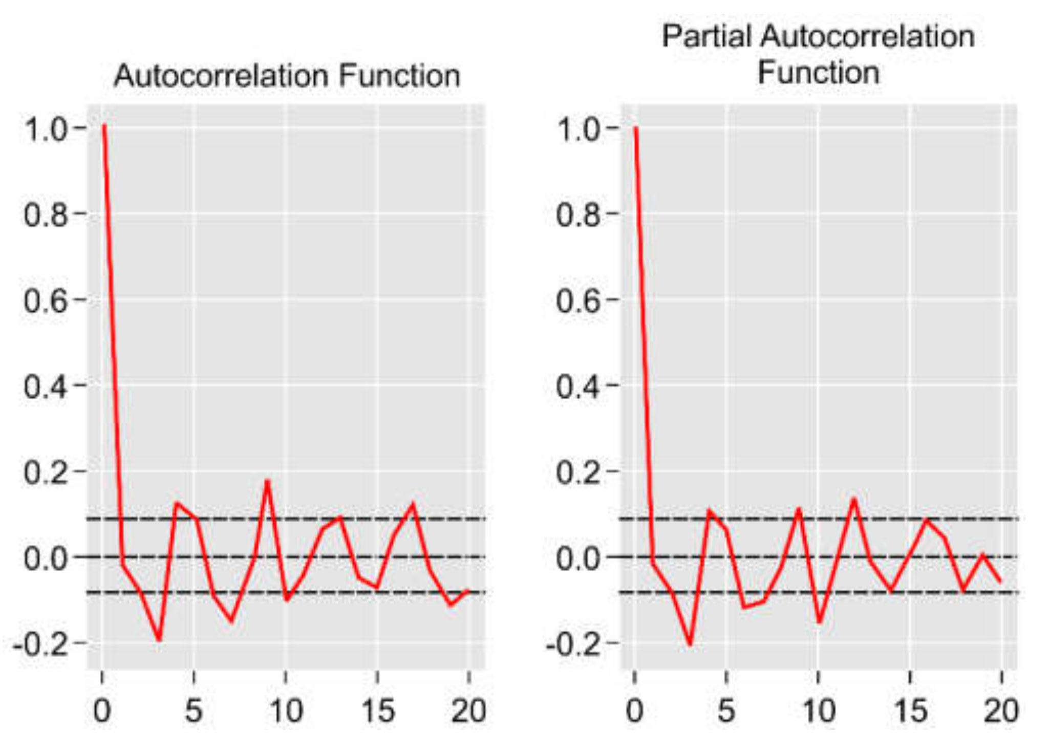
Box and Jenkins [31] proposed the use of the ACF and PACF of the sample data as the basic tools for identifying the order of an ARIMA model. The ACF is used to measure the amount of linear dependence between observations in a time series that are separated by a lag of $p$, whereas the PACF is used to determine the number of necessary autoregressive terms ($q$). Using this approach, it is possible to identify the preliminary values of $p$, $d$, $q$, $P$, $D$, and $Q$. Parameter $d$ is the order of the difference that depends on the stationarity of the time series. To assess stationarity, the order of differencing ($d$) needs to stationarize the series and remove the gross features of seasonality is determined; if $d=0$, the data do not tend to fluctuate over the long term, that is, the model is already stationary.

5.1.1. Autocorrelation Function (ACF)

The ACF is a measure of the correlation between a time series and a lagged version of itself. For instance, the ACF at a lag of five would compare the series at time instant ‘$“t_1”$… $“t_n”$ with the same series at ‘$“t_{1-5}”$… $“t_{n-5}”$ ($\mathrm{where} t_{1-5}$ and $t_{n-5}$ are the end points). The value of q was obtained from the ACF at $y=0$.

5.1.2. Partial Autocorrelation Function (PACF)

The PACF measures the correlation between a time series and a lagged version of itself after eliminating all variations that have already been explained by intervening comparisons. For example, the PACF at a lag of five checks the correlation described in Section Data Description. but removes the effects already explained by lags one to four. The value of $p$ was obtained from the PACF at $y=0$. Plots of the ACF and PACF are shown in Figure 3.

5.1.3. Parameters for SARIMA Model

The values used for the SARIMA model are summarized in

Table 4. Parameter ranges used for the SARIMA model.

	Non-Seasonal			Seasonal
Parameters	$p$	$Q$	$d$	$P$	$Q$	$D$
	3	1	2	0	1	1

.

5.2. The Proposed LSTM Architecture

The LSTM parameters include a sequence length, which determines how long the LSTM method should remember information and the dropout, that floats between zero and one. The method also counteracts overfitting and includes other parameters that control training. The values are listed in

Table 5. Values used for respective LSTM model parameters.

Parameter	Value
Sequence Length	120
Dropout	0.0 (do not drop for the linear transformation of the inputs)
Epochs	200
Input dimension	120
Activation Function	Tanh
Recurrent Activation Function	Sigmoid
Optimization Function	Adam
Loss	Mean squared error

. The LSTM model assessed in this study applied the mean-squared loss function over 200 epochs. Here, “epoch” is a hyperparameter, wherein one epoch corresponding to an iteration comprises one forward and one backward pass through the neural network model. Because an entire epoch is too large to be fed into a computer in one step, it is often divided into several smaller batches. We used Adam as our optimizer to control the number of iterations using an early stopping criterion [32].

We tested different parameters of the LSTM model, and the parameters that generated the best results were applied and reported for each freight index. The LSTM model used a neural network with one input layer, 120 hidden layers (dimensions), and one output layer.

5.3. Assessment Metric

The RMSE, which is often used to evaluate trained models for accuracy, is the standard deviation of the residuals or differences between the predicted and observed values. The formula for computing the RMSE is as follows:

$$\mathrm{RMSE}=\sqrt{\frac{1}{\mathrm{n}}{{\displaystyle \sum }}_{i=1}^{\mathrm{n}}{\left(y_i-{\widehat{y}}_i\right)}^2}$$

(9)

where n is the total number of observations, $y_i$ is the observed value, and ${\widehat{y}}_i$ is the predicted value. The main benefit of using the RMSE is that it penalizes large errors and scales the scores into the same units as the forecast values (i.e., per week for this study).

A smaller RMSE indicates a lesser noise and, therefore, a trained model with higher accuracy.

6. Results

The prediction algorithms were implemented using Python version 3.7.3 in MacOS Catalina (10.15.3, MacBook Pro; processor: 2.4 GHz Quad-Core Intel Core i5; memory: 16 GB, 2 × 133 MHz LPDDR3).

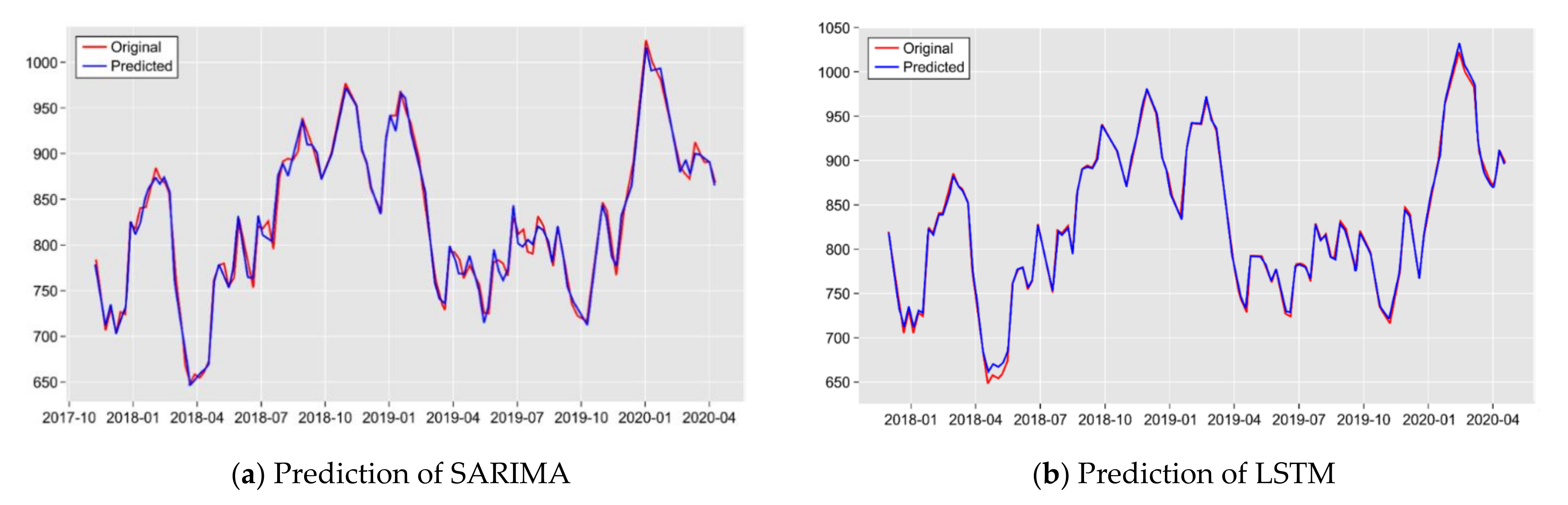
The selected SARIMA and LSTM models with the lowest predication errors were used to predict freight indices. Figure 4 shows the prediction of the comprehensive SCFI using SARIMA and LSTM.

We compared the results of different time steps and reported those that generated better performance. The results of the average RMSEs obtained using the rolling SARIMA and LSTM models, presented in

Table 6. RMSE results.

RMSE	SARIMA	LSTM	Time Steps	Reduction in RMSE
SCFI	49.13	17.62	5	64%
NCMP	124.26	28.43	9	77%
MED	129.84	39.01	9	70%
USWC	144.52	26.47	9	82%
USEC	140.00	20.97	4	85%
Persian	55.32	9.98	3	82%
ANZ	54.88	9.46	4	83%
WAF	110.38	22.45	7	80%
SAF	70.76	15.15	3	79%
SAM	223.80	32.58	3	85%
JPNW	3.19	7.75	9	−143%
JPNE	2.71	7.73	8	−185%
SEA	25.78	10.86	3	58%
KOR	7.66	6.99	3	9%

, indicate that for all major routes, the LSTM models significantly outperformed the SARIMA models. The highest forecasting error reduction was 85% for the SAM and SAF routes, reflecting the practices observed in current market. Deep-sea shipping routes (NCMP, MED, USWC, USEC, Persian, ANZ, WAF, SAF, and SAM) are of long distance, require large vessels and containers, and are limited in the number of companies that can participate. In addition, because of the high freight rates of these shipping routes, the majority of shipments are moved under fixed long-term freight contracts while the rest are moved under spot rates. Freight rates under the long-term contracts for these routes are fixed and generally lower than spot rates. Although the SCFI is an indicator of spot rates, shippers decide whether to carry cargo at spot or contract rates depending on market conditions. Therefore, both short-term changes and long-term trends in contracted freight rates affect spot rates.

LSTM is capable of capturing the patterns of both long-term trends such as yearly pattern and short-term trends such as weekly patterns, which explains why LSTM outperformed SARIMA in forecasting deep-sea shipping routes. In addition, deep-sea shipping routes, such as the Europe, America, South America, and South Africa routes, are subject to the influence of multiple expected and unforeseen factors. Deep-learning-based algorithms accommodating both long-term and short-term memories are therefore more suitable for this type of shipping route.

Notably, there were also two trade lanes, namely JPNW and JPNE, where the SARIMA models performed better than LSTM. For short-sea shipping routes, linear models, such as SARIMA, often generate better performance. In addition to the small proportion of long-term contracts, the effect of unanticipated factors is small, which can be attributed to the high explanatory power of the ordinary seasonal fluctuations.

For KOR, there was no significant improvement in the RMSE between the LTSM and SARIMA. These routes have shorter distances than other routes, with relatively large numbers of shipping companies and a few small companies participating. As a result, the average size of the ships in operation is small. For example, as of 2018, there were at least 40 companies on the route between Japan and China and at least 24 companies between China and Korea. The average vessel size is only approximately 1000 TEUs on the Japan–China and China–Korea routes. In addition, Chinese state-owned shipping companies occupy significant positions on all the routes. These carriers sometimes transport cargo without profit, and the base rates sometimes even fall below USD 0. Differences in market environments might influence the forecast accuracy of SARIMA and LTSM.

7. Discussions and Future Studies

Time-series forecasting has been a popular research topic in many fields over the past few decades. The accuracy of time-series forecasting is fundamental to many decision processes. Therefore, concerted efforts have been made to improve the accuracy of forecasting models. In addition to conventional econometric methods, the collection of machine-learning-based techniques for time-series forecasting has grown in recent years. However, there have been no comparative studies between conventional and machine-learning-based models in terms of their ability to forecast the comprehensive SCFI.

The authors of this study presented a deep-learning-based LSTM model for forecasting the SCFI. The results indicated that the LSTM model is effective in predicting freight-rate movement for deep-sea routes, which are easily affected by various factors during each voyage. For example, in predicting freight indices for South America and South Africa routes, LSTM reduced the forecasting error by 76% compared to an SARIMA model. However, for short-sea routes, the SARIMA models outperformed the LSTM models.

Our results are significant due to four major reasons. First, while the study complements the existing literature, LSTM has, to the best of our knowledge, not been previously applied to predict the SCFI.

Second, our results provide insights for improving forecasting accuracy. With the growing availability of large datasets and improvements in algorithms, deep-learning algorithms are becoming increasingly popular in many fields, including shipping. Determining the accuracy and power of these newly introduced approaches relative to conventional methods is of significant interest. The study showed that LSTM is superior to SARIMA in predicting the SCFI for some deep-sea routes and hence highlights the relative advantage of newly introduced approaches. One of the significant contributions of this study is that it highlights that the preferred method may depend on the market conditions of the shipping routes.

Third, our research findings can help relevant parties to understand the overall trends in the container shipping market. The SCFI is one of the most cited metrics for assessing the health and conditions of global trade. Global top carriers refer to the SCFI in their annual reports [33]. The composite SCFI reached its highest value of 5109 on 7 January 2022. This booming market is partially a result of decreased supply and increased demand owing to COVID-19 and the proliferation of e-commerce. During the COVID-19 crisis, carriers blanked large numbers of sailings, which led to a decrease in capacity. Further surges in the demand to prepare for the subsequent spread of infectious diseases have led to a worldwide lack of available container boxes. These conditions contribute to a state of market instability, and better prediction accuracy is essential for planning, managing, and optimizing the use of resources [4]. By offering a better forecasting model, our study provides governments, shippers, carriers, and analysts with insights into the mechanisms of container freight and the health of the container shipping industry.

Fourth, our results have implications for future investments. As the SCFI is often used as the underlying asset in freight derivatives, such as forward freight agreements (FFAs) [4], better predictions of the index would lead to better decision-making by the shipping industry, trading companies, and shippers regarding the use of freight derivatives to hedge against the volatility of freight rates.

Relevant data samples are still limited due to the short history of the SCFI. Future studies may focus on experimenting with other forecast techniques to further improve forecasting accuracy.