Article

Estimation and Analysis of JONSWAP Spectrum Parameter Using Observed Data around Korean Coast

1
Marine Bigdata Center, Korea Institute of Ocean Science and Technology, Busan 49111, Korea
2
Department of Civil and Environmental Engineering, Wonkwang University, Iksan 54538, Korea
3
Maritime ICT R&D Center, Korea Institute of Ocean Science and Technology, Busan 49111, Korea
4
Department of Applied Ocean Science, KIOST School, Korea University of Science and Technology, Busan 49111, Korea
5
Ocean Science and Technology, Korea Maritime and Ocean University, Busan 49111, Korea
*
Author to whom correspondence should be addressed.
J. Mar. Sci. Eng. 2022, 10(5), 578; https://doi.org/10.3390/jmse10050578
Submission received: 6 March 2022 / Revised: 8 April 2022 / Accepted: 19 April 2022 / Published: 25 April 2022
(This article belongs to the Section Coastal Engineering)

Abstract

:
The relationship between significant wave height ( H 1 / 3 ) and period ( T 1 / 3 ) was obtained using wave data from the East and Yellow coasts of the Korean Peninsula to facilitate the calculations of the wave parameters. In addition, the JONSWAP spectral parameters were estimated and analyzed for all wave height ranges. The relational expression between the two wave variables ( H 1 / 3 ~ T 1 / 3 ) obtained from this study showed a significant difference from the previously proposed relational expressions, most of which tended to follow the lower limit of the data. Meanwhile, the suggested peak enhancement factor (PEF,   γ ) is 1–7; however, for this study, a peak control factor (PCF,   γ c ) with a range of 0–10 was introduced. As a result of the analysis, the PCF was determined to be 1.13–1.42, which is approximately 40% smaller than the previously proposed γ   =   3.3 . The probability density distribution of the appropriate PCF was then calculated, and the gamma and log-normal distributions for the East and Yellow coasts of the Korean Peninsula were found, respectively. This study covered waves of all range heights, and the analysis results can be used as important data to explain the characteristics of the sea area.

1. Introduction

The ocean has abundant resources; as the interest in it is increasing, analyzing and understanding the nature of waves is important. However, waves consist of a combination of components that are continuously changing, depending on the time and location. Waves can be expressed as a spectrum, and the energy density distribution of the waves can be determined through statistical analysis. Therefore, a spectrum of ocean waves is widely used when analyzing irregular waves. The wave spectrum is typically given as a parameterized function. Spectral models include the PM (Pierson–Moskowitz) [1] and BM (Bretschneider–Mitsuyasu) spectrums [2,3] for fully grown wind waves; JONSWAP (Joint North Sea Wave Observation Project) [4] and TMA spectrums [5] for deep sea and finite water depth; and Wallops spectrum [6] for shallow waters. Several studies have been conducted to reproduce and parameterize the wave spectrum in various regions [7,8,9,10,11,12]. However, the previously proposed wave spectrum uses parameters to which the wave characteristics of the target analysis area are applied, and it is very important to change these parameters to estimate the optimal wave parameters suitable for the area of interest. Research on estimating the peak enhancement factor (PEF, γ ) of the JONSWAP spectrum is being actively conducted. Feng et al. [13] suggested an optimal PEF in the range of 3.43–3.70 for the Jiangsu waters in China. Jamal et al. [14] proposed a wave spectrum range based on the peak frequency ( f p ) through a comparative analysis using the JONSWAP spectrum for the Sabah and Sarawak waters in Malaysia. Saulnier [15] found that the estimated PEF from curve-fitting spectra were biased between 5% and 30%, depending on the sample record length, peak frequency, and PEF. Mazaheri and Imani [16] defined the JONSWAP spectral parameters as a function of the significant wave height ( H s ) and peak frequency ( f p ), rather than a simple numerical value, for the coast of the Persian Gulf. Ewans and McConochie [17] proposed a method to simultaneously obtain the peak augmentation coefficient and bandwidth representing the spectrum width through sensitivity analysis to calculate the uncertainty of the estimated JONSWAP parameters. Furthermore, Ewans and McConochie [18] proposed an optimal technique for estimating the PEF of the JONSWAP spectrum to design offshore structures using hindcast data. Rueda-Bayona and Guzman (2020) [19] also performed alpha and gamma parameter estimation of the JONSWAP spectrum using the GA model (Genetic Algorithms Model).
In Korea, Cho et al. [20] estimated that γ   =   1.4 using the wave spectrum data observed in Namhangjin. Kang and Lee [21] reported that γ   =   2.07 by the parameters of the JONSWAP spectrum, using the autumn–winter observation data of the northeastern coast of Jeju. Suh et al. [22,23] found that γ   =   2.14 using various wave observations and retrospective data off the coast of the Korean Peninsula and proposed a form of probability density distribution for γ .
However, in most of these studies, it was difficult to acquire long-term data; therefore, most analyses were performed using data obtained through numerical models and hydraulic experiments. In addition, an appropriate method was required to estimate the JONSWAP spectrum parameters from the long-term observational data. Most of the wave spectrum analysis methods are performed in regions with high wave heights, owing to advantages such as the reliability of spectrum data and structural designs. However, as the utilization of marine space such as wave power generation has increased in recent years, there is a need to analyze the target sea area in detail for all wave heights. In this study, the relationship between the significant wave height ( H 1 / 3 ) and wave period ( T 1 / 3 ) was analyzed using wave data from the coast of the Korean Peninsula. Moreover, the concept of a peak control factor (PCF, γ c ) was proposed by adjusting the range of the PEF ( γ ), which determines the peak of the JONSWAP spectrum for all wave height ranges, and the optimal PCF value and probability density distribution were determined.

2. Materials and Methods

2.1. Observation Data

In this study, the wave characteristics of the Korean Peninsula were analyzed using wave data observed at four points on the East Sea coast and two points on the Yellow Sea coast, as shown in Figure 1. On the East Sea coast, wave observations were performed using an acoustic wave and current profiler (AWAC) in Gonghyeounjin (GHJ), Maengbang (MB), and Hupo (HP), while a signature acoustic doppler current profiler (Signature ADCP 500) was used in Ulsan New Port (USN). The Herald of Meteorological and Oceanographic Special Research Units (HeMOSU-1 and HeMOSU-2) on the Yellow Sea coast used waveguide equipment installed in oceanographic and meteorological observation towers (Figure 1 and Table 1).
The AWAC and signature ADCP 500 equipment used on the East coast contained an ultrasonic wave meter developed by Nortek, Norway. This equipment collected 2048 water surface fluctuation data points every 0.5 s and stored them inside the device, and then it calculated the wave parameters through wave train and spectrum analysis using Storm 64 software. For the wave train analysis, the zero-crossing method was applied; for the wave spectrum analysis, after applying the fast Fourier transform (FFT), wave information was calculated through kernel smoothing. The standard of the wave period applied for a wind wave was 0.5–30 s, and the calculated wave information, such as the significant wave height ( H s or H 1 / 3 ), peak wave period ( T p ), and wave period ( T 1 / 3 ), were recorded every 30 min [24]. The waveguide equipment used on the Yellow coast was developed using Delft, with an observation interval of 5 Hz (200 ms) to collect the water surface elevation information. The accuracy of the wave train analysis method was evaluated in time domain using the observed water surface elevation data. The wave spectrum analysis method was carried out in the standard wave analysis package (SWAP) software [25]. When using SWAP, after correcting the observation data through a 10% cosine window, a spectrum analysis in the frequency domain was performed using the FFT to calculate the wave parameters. Figure 2 presents examples of the water surface elevation data observed at the HeMOSU-2 station and the frequency spectrum shape calculated using FFT.

2.2. Method

Significant wave height and wave period are important wave parameters for understanding the wave characteristics of the targeted sea area and are mainly used in the design of harbors and coastal structures. Although these parameters are determined based on wave estimation, the two maintain a relationship during the wave development and attenuation. In general, the relationship between the significant wave height and significant wave period can be expressed as T 1 / 3 ξ ( H 1 / 3 ) τ . Suh et al. [23] proposed the relationship T 1 / 3 6.21 ( H 1 / 3 ) 0.32 , T 1 / 3 6.65 ( H 1 / 3 ) 0.23 , and T 1 / 3 5.59 ( H 1 / 3 ) 0.20 for Pohang, Busan, and Hongdo, respectively, which are similar to the areas of interest at Hupo, Ulsan New Port, and HeMOSU, which are to be analyzed in this study. In addition, Jeong et al. [26] suggested the relation T 1 / 3 6.50 ( H 1 / 3 ) 0.22 for Namhangjin on the East coast of the Korean Peninsula, the location similar to that of Gonghyeonjin and Maengbang, which are also among the areas of interest of this study. Goda [27] proposed the relation T 1 / 3 3.3 ( H 1 / 3 ) 0.63 from Wilson’s wave estimation equation for waves developed by wind, and T 1 / 3 3.85 ( H 1 / 3 ) 0.5 in the Shore Protection Manual (abbreviated as SPM hereinafter) [28]. In this study, the relationship between the significant wave height and wave period was estimated using the obtained observational data, and the values of ξ and τ, calculated using curve fitting and a non-linear least squares method, are compared with those of Goda [27] and SPM [28] among the relational equations previously proposed.
The JONSWAP spectrum is a spectrum distribution proposed by applying the PCF ( γ ) to the Pierson-Moskowitz spectrum, in turn proposed using the existing Philips parameters and peak frequency ( f p ), and is expressed as follows (see Equations (1)–(3)):
S J ( f ) = α g 2 ( 2 π ) 4 f 5 exp [ 1.25 ( T p f ) 4 ] γ p *   ;
p * = exp [ ( T p f 1 ) 2 2 σ 2 ]   ;
σ     { σ a = 0.07 , f     f p σ b = 0.09 , f > f p   ;
where the Philips parameter α = 0.0081 . However, in this study, the JONSWAP equation proposed by Goda [29] as a function of significant wave height and peak wave period was used as shown in the following Equations (4)–(6):
S J ( f ) = B J H 1 / 3 2 T p 4 f 5 exp [ 1.25 ( T p f ) 4 ] γ p * ;
B J     0.0624 ( 1.094 0.01915 × l n γ ) 0.230 + 0.0336 γ 0.185 ( 1.9 + γ ) 1   ;  
T p = T 1 / 3 / [ 1 0.132 ( γ + 0.2 ) 0.559 ] ;
In general, the parameter of the JONSWAP spectrum is called the PEF ( γ ) and is applicable when γ   1.0 . However, although the JONSWAP spectrum has been proposed as a spectrum applicable to high-frequency regions in the North Sea, the range of use has recently been diversified, and it is necessary to analyze the accuracy of using the JONSWAP spectrum for a normal wave (which has a significant wave height of approximately 1 m). Therefore, the purpose of this study is to consider the parameters of the JONSWAP spectrum for all significant wave height ranges as defined in Equation (7). In general, when the range of γ was γ     1.0 m , it is defined as the PEF. If γ < 1.0   m , it is classified as the peak reduction factor. In this study, we propose a PCF (range: γ c > 0 ) as a parameter of the JONSWAP spectrum.
To estimate the γ c of the JONSWAP spectrum, the range of γ c was changed from 0.05 to 10 with a step length of 0.05, and the RMSE of the observed and estimated spectrum was calculated as in Equation (8) to calculate the γ c value with the smallest error.
γ c ( P e a k   C o n t r o l   F a c t o r ) = { P e a k   E n h a n c e m e n t   F a c t o r   ( γ     1 ) , P e a k   R e d u c t i o n   F a c t o r   ( γ < 1 ) .
RMSE   = k = 1 n [ S ^ ( f k ) S ( f k ) ] 2 n .
where S ^ ( f k ) is the observed wave spectrum, and S ( f k ) is the estimated wave spectrum. In addition, in Figure 3, examples of the meaning of the parameters of the JONSWAP spectrum described above and the changes in the spectrum shape according to the variations in PEF and PCF are presented.

3. Result and Discussion

3.1. Relationship between Significant Wave Height and Wave Period

The results of the analysis of the relationship between the significant wave height ( H 1 / 3 ) and the significant wave period ( T 1 / 3 ), calculated using the wave train analysis, are shown in Figure 4. The variability of the significant wave period was higher than that of the significant wave height. As the wave height decreased, a large period appeared owing to a long-period component such as swell. However, the previously proposed equations of Goda [27] and SPM [28] followed the lower limit of the observation data at all points and tended to be underestimated. There is a difference between the two proposed equations because they are proposed for regions where wind waves are dominant, and this trend is similar to the results of many previous studies [23,30,31]. In addition, the relationship between the significant wave height and period at GHJ, MB, HP, and USN located in the East Sea had a larger distribution of data than that of HeMOSU-1 and -2 located in the Yellow Sea ( ξ was estimated to be approximately 15% larger). This is due to the influence of the wave environment characteristics on the sea area, such as typhoons and monsoons.

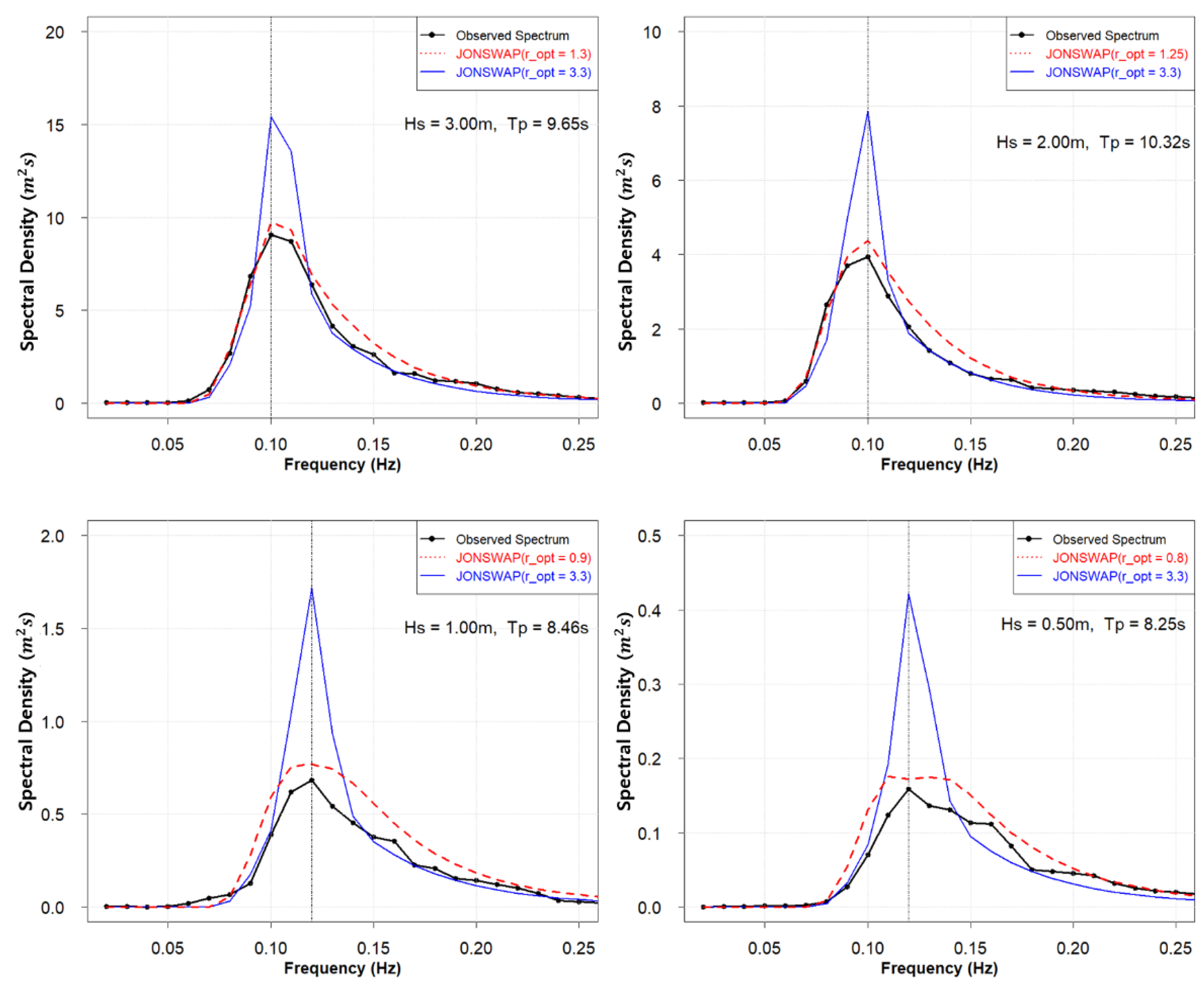
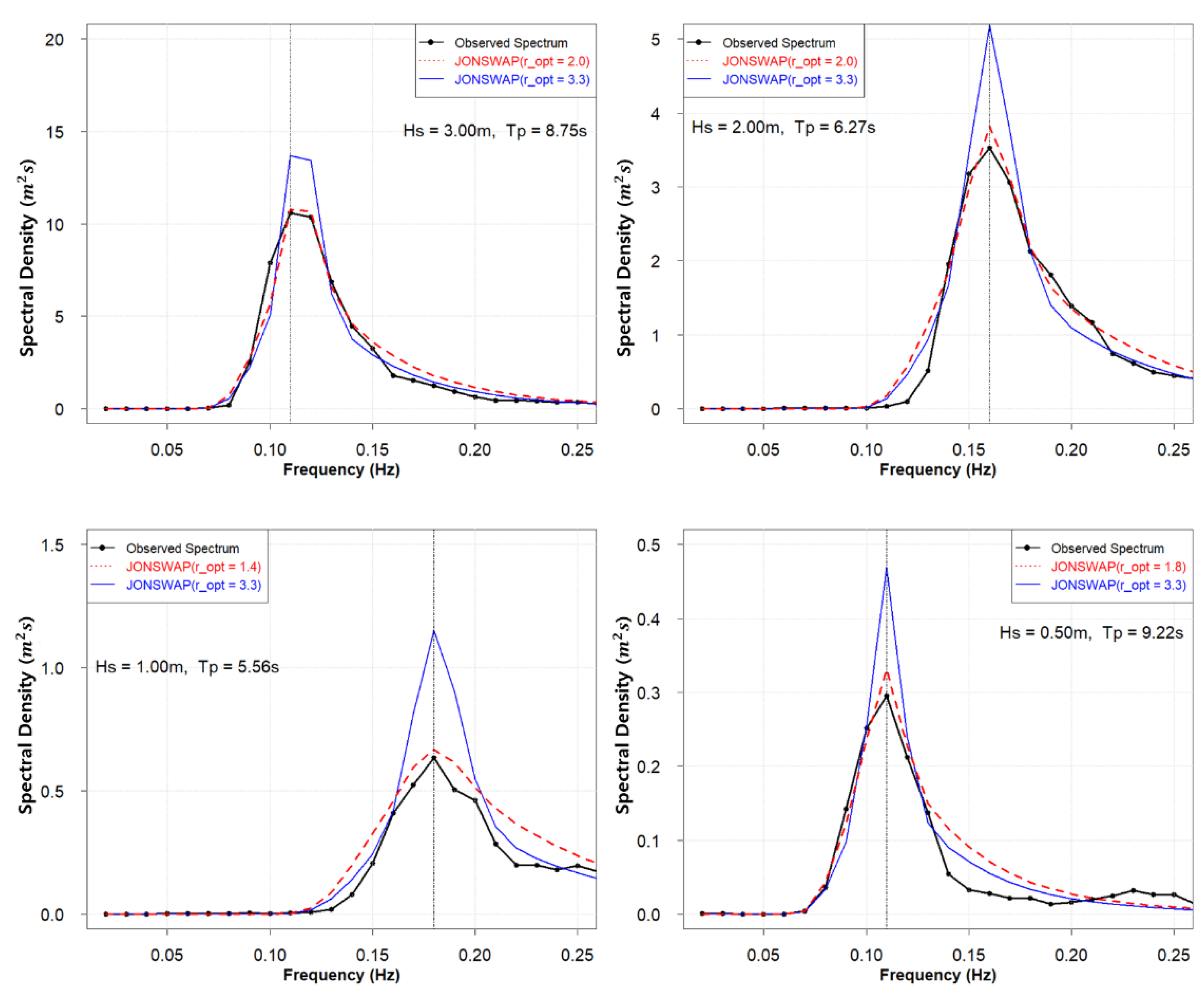
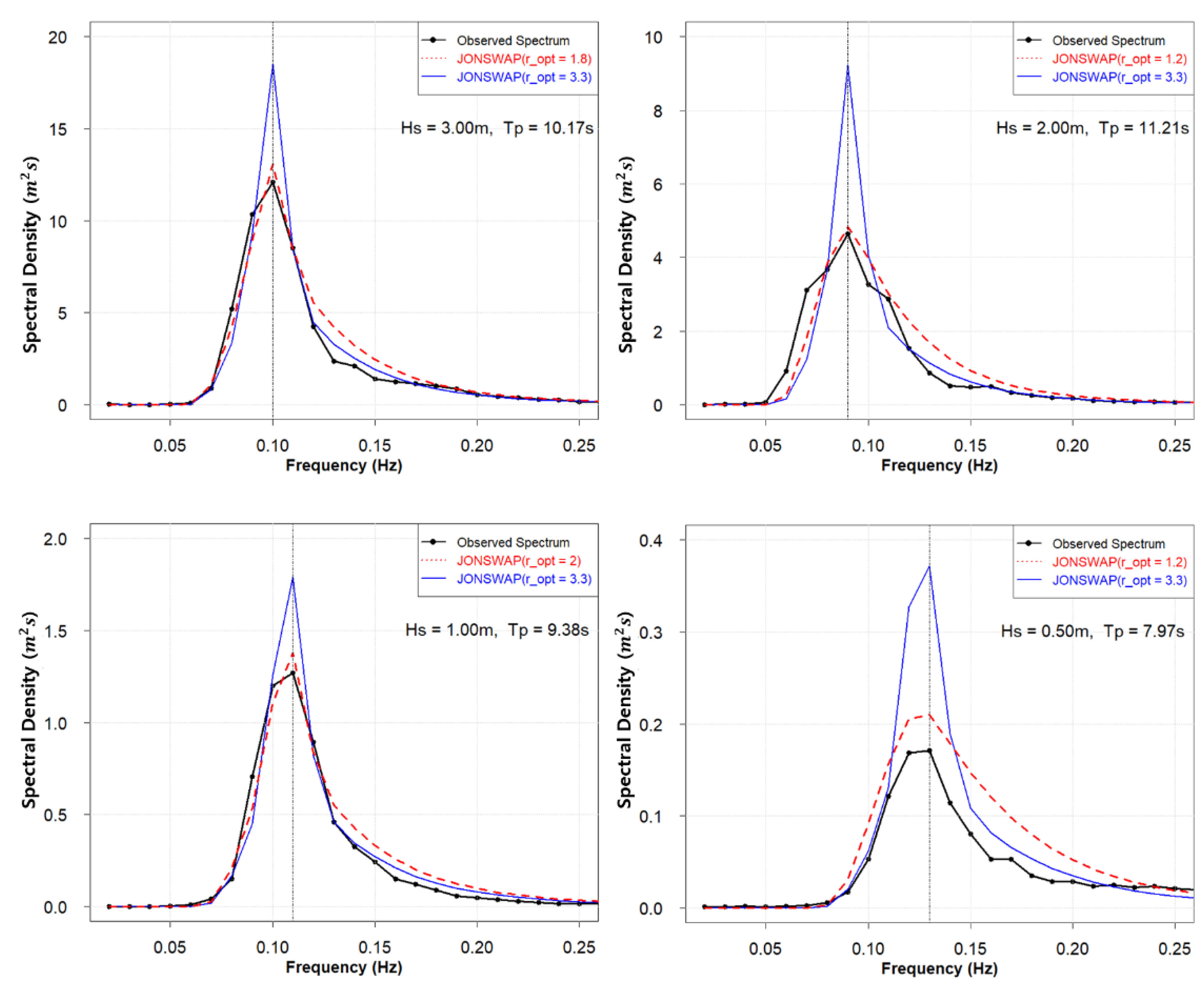
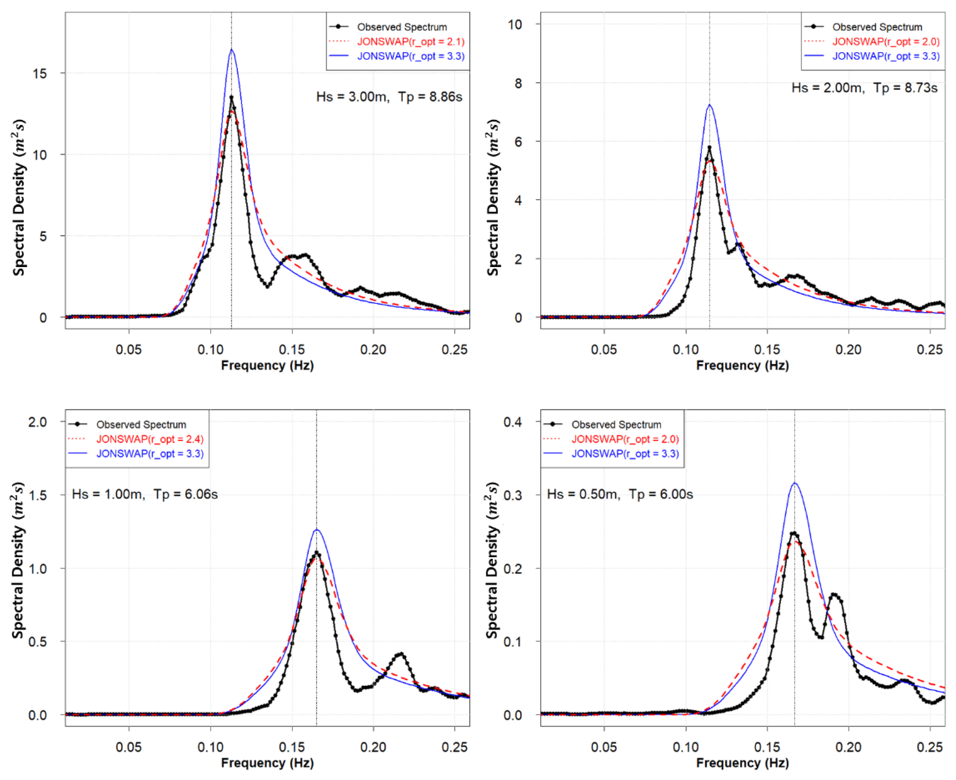
3.2. Estimation of JONSWAP Spectrum Parameter

The results of estimating the PCF ( γ c ) of the JONSWAP spectrum for all the wave height ranges are presented in Figure 5 and Table 2. In general, in the JONSWAP spectral distribution equation, the γ c ¯ (mean of PCF) of all points was 1.13–1.42, which is approximately 40% smaller than that obtained by applying γ = 3.3 in the high wave height range for PEF. In addition, as the range of PCF decreased with the increasing wave heights, it converged to the average of γ c , and γ c ,   m a x was calculated to be in the range of H s < 1.0   m at all sites except for the HeMOSU-2 station. Considering the PCF, according to the range of wave heights, there was no significant difference in the average PCF of each section, and most of them were distributed between 1 and 2. However, the PCF showed a gradual increase in dispersion, indicating the range of the PCF as the wave height decreased. This is considered a limitation in estimating the appropriate PCF because most of the wave heights are distributed below 1.0 m, and the growth of wind waves is not sufficient (see Figure A1, Figure A2, Figure A3, Figure A4, Figure A5 and Figure A6 in Appendix A).
The results of comparing the observed spectrum with the PCF calculated in this study are presented in Figure 4, and the spectrum to which γ = 3.3 was used for further comparison. As a result of the analysis, the spectrum estimated using γ = 3.3 suggested by the JONSWAP spectrum (Figure 4, blue line) tended to be overestimated by up to 50%, and this trend was similar to the study results of Xie et al. [32]. The JONSWAP spectrum (Figure 6, red dot), estimated by applying the optimal PCF calculated in this study, showed a similar trend to the observed spectrum. In addition, as shown in Figure A7, Figure A8, Figure A9, Figure A10, Figure A11 and Figure A12 in Appendix A, there were cases where the PCF was applied as a value of 1.0 or less in the range of wave heights below 1.0 m. It was determined that there was a limitation in performing the proper estimation of the JONSWAP spectrum for the observed spectrum at such a low wave height. To solve this problem, it is necessary to improve the accuracy of the estimated spectrum by calculating σ , a coefficient that determines the interval of the JONSWAP spectrum, simultaneously with the PCF.
The probability density function of the PCF, which is a parameter of the JONSWAP spectrum, is presented in the form of a log-normal distribution and normal distribution functions, as shown in Equations (9) and (11) [23,32]. In this study, the distribution fit was determined for the log-normal, gamma, normal, and Weibull distribution functions using the PCF calculated for all wave height ranges.
-
Log-normal distribution
f ( γ c ;   μ ,   σ ) = 1 2 π σ γ c exp ( ( l n γ c μ ) 2 2 σ 2 )
where μ is mean, and σ is the standard deviation
-
Gamma distribution
f ( γ c ; k ,   θ ) = 1 θ k Γ ( k ) γ c k 1 e γ c θ
-
Normal distribution
f ( γ c ;   μ ,   σ ) = 1 2 π σ exp ( ( γ c μ ) 2 2 σ 2 )
-
Weibull distribution
f ( γ c ; k ,   θ ) = ( θ k ) ( γ c k ) θ 1 exp [ ( γ c k ) θ ] ( γ c 0 ; k ,   θ > 0 )
In Equations (10) and (12), k is shape parameter, and θ is scale parameter.
In addition, to estimate the optimal distribution, the probability density distribution and distribution fit test of the PCF were performed using the p-value calculated using the KS test (Kolmogorov–Smirnov Tests). However, because the KS test calculates even small, meaningless differences such as both ends of the probability density distribution, there was a limit to the appropriate distribution difference test. Accordingly, in this study, a distribution similar to the PCF probability density distribution was estimated using the average of the calculated p-values after randomly sampling 1% of the calculated PCF data and repeating the calculation 1000 times [33]. Then, as shown in Equation (13), the optimal distribution in which the difference between each probability density distribution is minimized was determined using the Kullback–Leibler divergence (KL divergence) (Figure 7). The KL divergence is a method used to calculate the difference between the distribution of the observed and estimated spectrums; the smaller the D K L value, the more similar the two distributions [34].
D K L ( P | | Q ) = i P ( i ) l o g P ( i ) Q ( i )
where P ( i ) is the observed spectrum, and Q ( i ) is the estimated spectrum.
As shown in Figure 5, most of the analysis target sites showed a form similar to the log-normal and gamma distributions. The KS test was adopted at the 95% significance level, and both the normal and Weibull distributions were rejected. However, the KS test is used to determine the fit for each distribution and is limited in estimating the optimal probability density distribution. In addition, more rigorous testing is required for errors and distribution fits at the extreme end of the distribution, which is highly sensitive to probability values. Therefore, to estimate the probability density distribution that is most similar to γ c , KL divergence analysis was performed to quantitatively measure the difference between the distributions of the two probabilities.
Consequently, the smallest value for D K L was calculated in the gamma distribution for GHJ, MB, HP, and USN located on the East coast of the Korean Peninsula and in the log-normal distribution for H1 and H2, located on the Yellow coast of the Korean Peninsula. There was also a difference in the probability density distribution of γ c based on the sea area of the Korean Peninsula.

4. Conclusions

In this study, wave analysis was performed using wave observation data from four and two points on the East and Yellow coasts of the Korean Peninsula, respectively. In the design of offshore structures, the relationship between the significant wave height and wave period, which can provide essential information when determining the design wave corresponding to the reproduction period, was calculated. In addition, the PCF ( γ c > 0 ), one of the parameters of the JONSWAP spectrum, was calculated for all wave height ranges, and the optimal PCF distribution was estimated.
The main conclusions of this study are as follows:
(1)
The relationship between the significant wave height and wave period proposed by Goda [27] and SPM [28], which is commonly used, tends to follow the lower limit at all points. In addition, in the calculated relational expression, ξ and τ were approximately 2 and 0.5 times different, respectively. When determining the design wave height, it is difficult to use the previously proposed relational formula, and the relationship between the significant wave height and period should be sufficiently understood using the observational data of the target sea area.
(2)
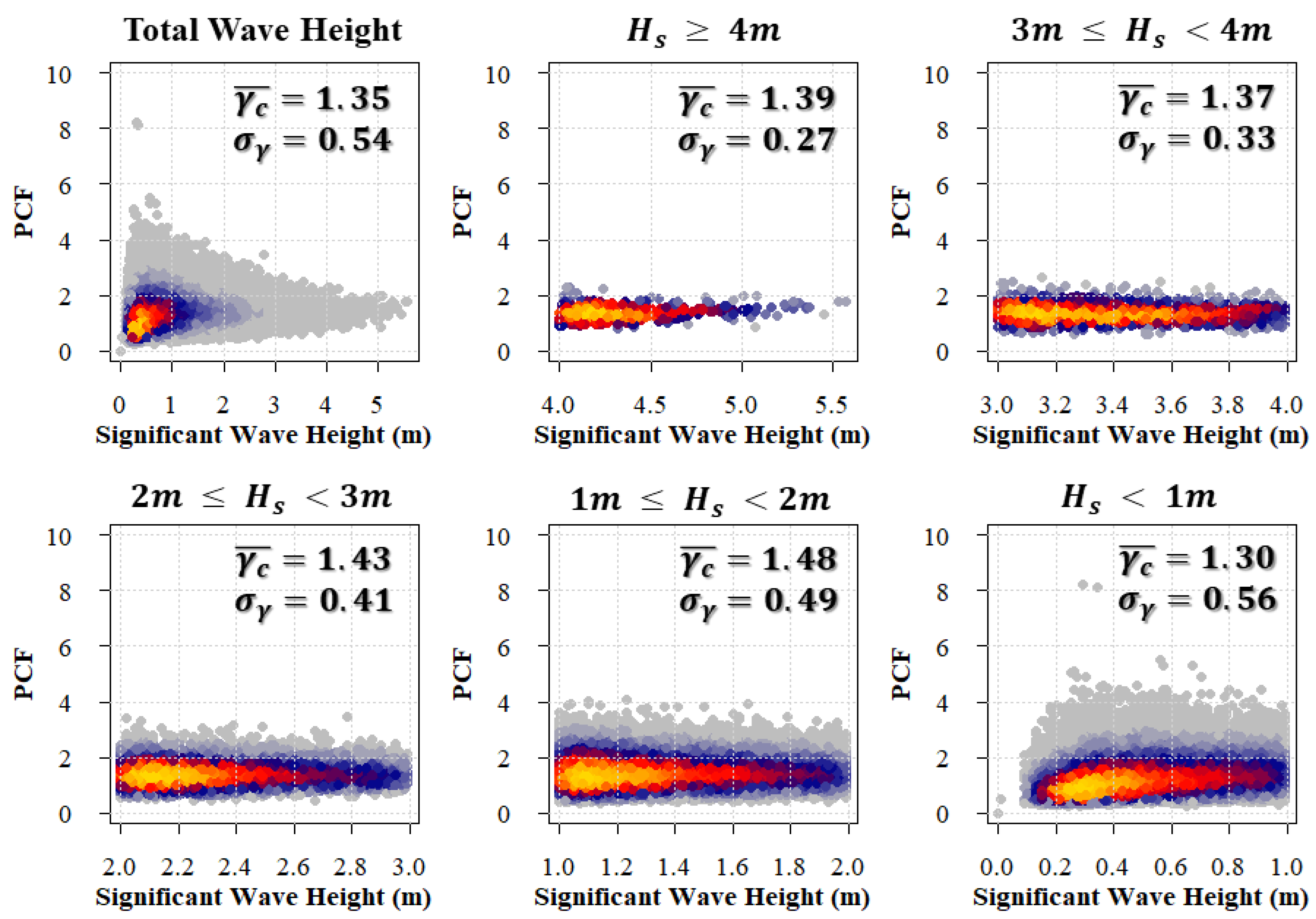
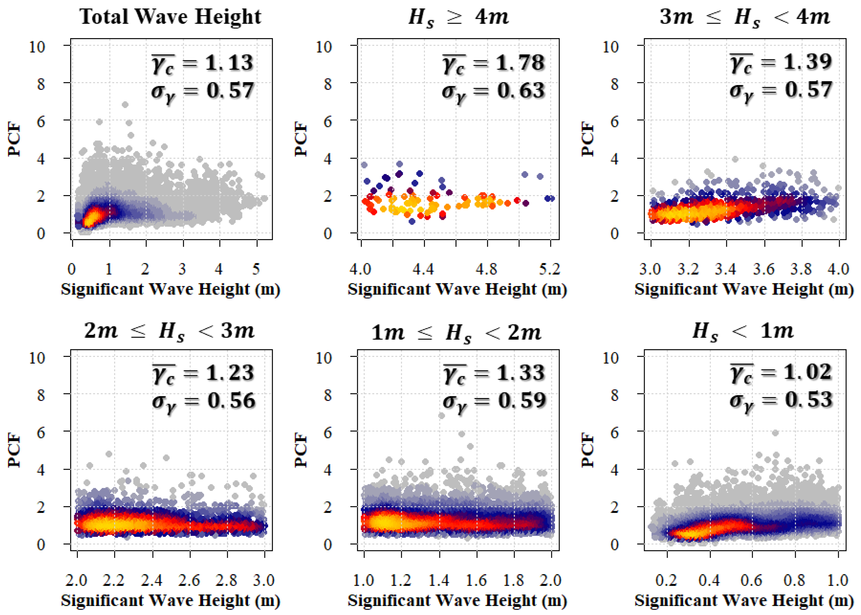
PCF estimated using the observation data for all six sites were found to be approximately 40% smaller, with γ c ¯ = 1.13 1.42 , than the previously reported PCF, γ c = 3.3 . The JONSWAP spectrum can be applied to waves with large height ranges. Therefore, as a result of calculating PCF in the H s   4.0   m region, which is considered to be a high-frequency region, γ c ¯ = 1.40 2.1 was obtained, showing a difference of up to 58% from the previously reported value. In addition, as the wave height decreased, the dispersion of γ c increased, and γ c for each section was distributed between approximately 1.0 and 2.0.
(3)
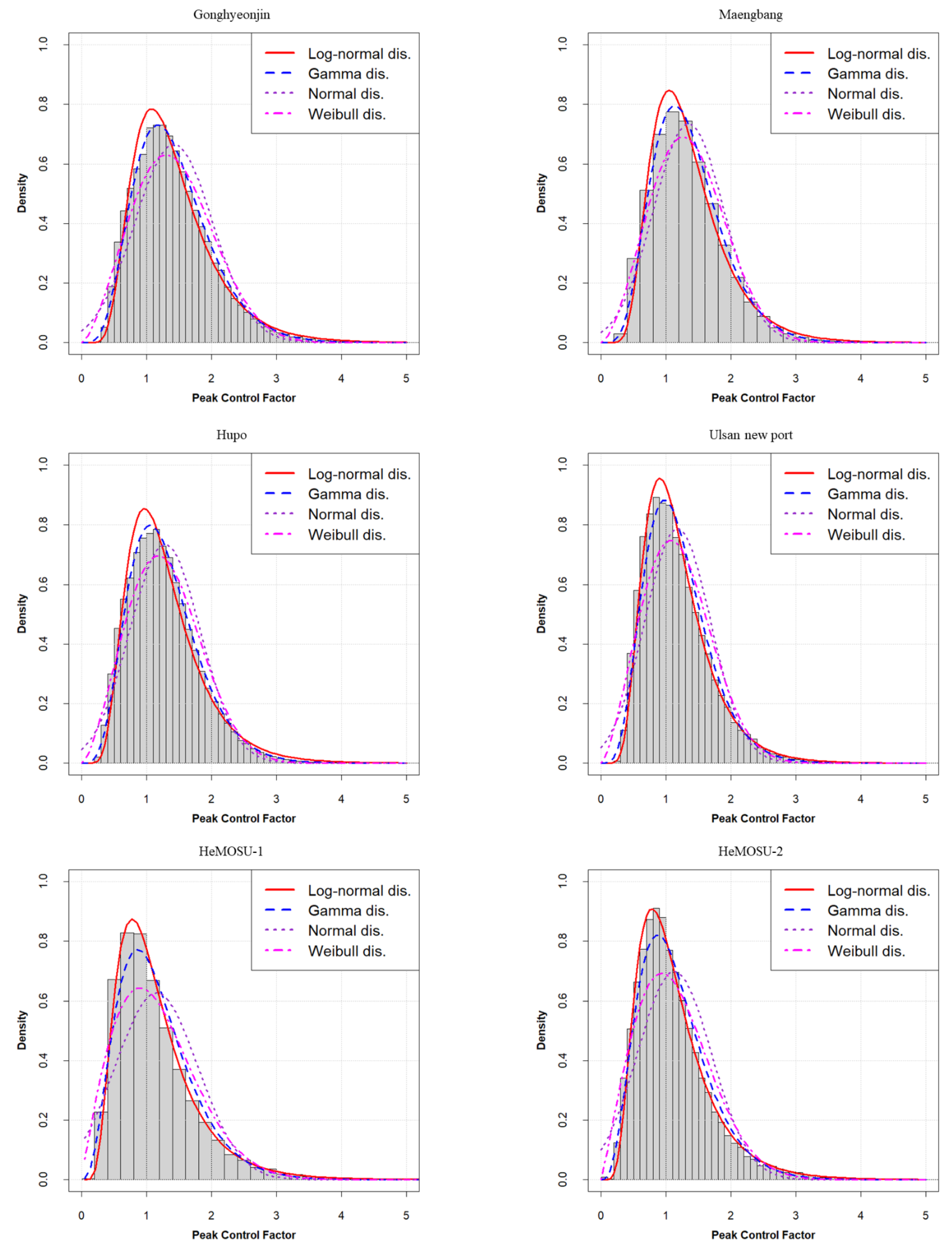
As shown in Figure 5 and Table 3, the probability density distribution of γ c , calculated by applying the distribution fit test and KL divergence method, showed differences amid the sea areas of the Korean Peninsula. In the case of the East and Yellow coasts of the Korean Peninsula, the gamma and log-normal distributions, respectively, were calculated as the most similar distributions, showing a significant difference from the normal and Weibull distributions.
The results calculated through the wave spectrum parameter estimation study are an important factor in designing coastal and offshore structures. In using the previously proposed parameters, temporal and spatial verification is required, which, however, is not conducted due to the limitations of ocean observation data. In this study, a single parameter of the JONSWAP spectrum was analyzed in various ways. However, it is necessary to improve the accuracy of the spectrum by simultaneously estimating various parameters for all wave height ranges, such as bandwidth control parameters ( σ ) and peak frequency ( f p ), within the spectrum. In addition, since the observed depth is in the range of about 13–30 m, the effect on the deep water was not considered, so it is considered that there is a limit to the application of the results of this study to the deep-sea area. If long-term observational data for various points and water depths are secured and analyzed, reliable results applicable to offshore structure design can be derived.

Author Contributions

Conceptualization, H.-Y.C. and U.-J.L.; methodology, H.-Y.C. and U.-J.L.; software, H.-Y.C. and U.-J.L.; validation, H.-Y.C. and U.-J.L.; formal analysis, U.-J.L.; investigation, W.-M.J.; resources, W.-M.J.; data curation, W.-M.J.; writing—original draft preparation, U.-J.L.; writing—review and editing, H.-Y.C. and U.-J.L.; visualization, U.-J.L.; supervision, H.-Y.C. All authors have read and agreed to the published version of the manuscript.

Funding

This research was funded by the Ministry of Oceans and Fisheries, grant number PG52810.

Conflicts of Interest

The authors declare no conflict of interest.

Appendix A

PCF Distribution Pattern for Each Significant Wave Height Range.
Figure A1. Gonghyeonjin (GHJ).
Jmse 10 00578 g0a1
Figure A2. Maengbang (MB).
Jmse 10 00578 g0a2
Figure A3. Hupo (HP).
Jmse 10 00578 g0a3
Figure A4. Ulsan new port (USN).
Jmse 10 00578 g0a4
Figure A5. HeMOSU-1 (H1).
Jmse 10 00578 g0a5
Figure A6. HeMOSU-2 (H2).
Jmse 10 00578 g0a6
Comparison of JONSWAP Spectrum Fitting between Observed Data; Estimated Spectra with Optimized γ c and Estimated Spectra with γ c = 3.3 .
Figure A7. Gonghyeonjin (GHJ).
Jmse 10 00578 g0a7
Figure A8. Maengbang (MB).
Jmse 10 00578 g0a8
Figure A9. Hupo (HP).
Jmse 10 00578 g0a9
Figure A10. Ulsan new port (USN).
Jmse 10 00578 g0a10
Figure A11. HeMOSU-1 (H1).
Jmse 10 00578 g0a11
Figure A12. HeMOSU-2 (H2).
Jmse 10 00578 g0a12

References

  1. Pierson, W.J.; Moskowitz, L. A proposed spectral form for fully developed wind seas based on the similarity theory of S. A. Kitaigorodskii. J. Geophys. Res. 1964, 69, 5181–5190. [Google Scholar] [CrossRef]
  2. Mitsuyasu, H. On the Growth of Wind-Generated Waves (2)—Spectral Shape of Wind Waves at Finite Fetch. In Proceedings of the 17th Japanese Conference, Kyoto, Japan, 16–21 October 1970; Available online: https://cir.nii.ac.jp/crid/1573105975214720000 (accessed on 5 March 2022).
  3. Bretschneider, C.L. Significant waves and wave spectrum. In Ocean Industry; Gulf Publishing Company: Houston, TX, USA, 1968; pp. 40–46. [Google Scholar]
  4. Hasselmann, K.; Barnett, T.P.; Bouws, E.; Carlson, H.; Carwright, D.E.; Enke, K.; Ewing, J.A.; Gienapp, H.; Hasselmann, D.E.; Kruseman, P.; et al. Measurements of windwave growth and swell decay during the Joint North Sea Wave Project (JONSWAP). Dtsch. Hydrogr. Z. 1973, 8, 1–95. [Google Scholar]
  5. Tucker, M.J. Nearshore waveheight during storms. Coast. Eng. 1994, 24, 111–136. [Google Scholar] [CrossRef]
  6. Huang, N.E.; Long, S.R.; Tung, C.C.; Yuen, Y.; Bliven, L.F. A unified two-parameter wave spectral model for a general sea state. J. Fluid Mech. 1981, 112, 203–224. [Google Scholar] [CrossRef]
  7. Kumar, V.S.; Kumar, K.A. Spectral characteristics of high shallow water waves. Ocean Eng. 2008, 35, 900–911. [Google Scholar] [CrossRef]
  8. Young, I.R. Observations of the spectra of hurricane generated waves. Ocean Eng. 1998, 25, 261–276. [Google Scholar] [CrossRef]
  9. Young, I.R. A review of the sea state generated by hurricanes. Mar. Struct. 2003, 16, 201–218. [Google Scholar] [CrossRef]
  10. SanilKumar, V.; Mandal, S.; Anand, N.M.; Nayak, B.U. Spectral representation of measured shallow water waves. In Proceedings of the Indian National Conference on Harbour and Ocean Engineering, Pune, India, 8–10 June 1994; Volume I, pp. 23–32. [Google Scholar]
  11. Kumar, V.S.; Anand, N.M.; Kumar, K.A.; Mandal, S. Multipeakedness and groupiness of shallow water waves along Indian coast. J. Coast Res. 2003, 1052–1065. [Google Scholar]
  12. Baba, M.; Dattatri, J.; Abraham, S. Ocean Wave Spectra Off Cochin, West Coast of India; Evisa: New Delhi, India, 1989. [Google Scholar]
  13. Feng, W.B.; Yang, B.; Cao, H.J.; Ni, X.Y. Study on wave spectra in south coastal waters of Jiangsu. In Applied Mechanics and Materials; Trans Tech Publications Ltd.: Freienbach, Switzerland, 2012; Volume 212, pp. 193–200. [Google Scholar]
  14. Amurol Jamal, S.; Ewans, K.; Sheikh, R. Measured Wave Spectra Offshore Sabah & Sarawak, Malaysia. In Offshore Technology Conference-Asia; OnePetro: Kuala Lumpur, Malaysia, 2014. [Google Scholar]
  15. Saulnier, J.B. Uncertainty in peakedness factor estimation by JONSWAP spectral fitting from measurements. In International Conference on Offshore Mechanics and Arctic Engineering (Vol. 55393, p. V005T06A001); American Society of Mechanical Engineers: New York, NY, USA, 2013. [Google Scholar]
  16. Mazaheri, S.; Imani, H. Evaluation and modification of JONSWAP spectral parameters in the Persian Gulf considering offshore wave characteristics under storm conditions. Ocean Dyn. 2019, 69, 615–639. [Google Scholar] [CrossRef]
  17. Ewans, K.; McConochie, J. On the Uncertainties of Estimating JONSWAP Spectrum Peak Parameters. In International Conference on Offshore Mechanics and Arctic Engineering (Vol. 51227, p. V003T02A034); American Society of Mechanical Engineers: New York, NY, USA, 2018. [Google Scholar]
  18. Ewans, K.; McConochie, J. Optimal methods for estimating the JONSWAP spectrum peak enhancement factor from measured and hindcast wave data. J. Offshore Mech. Arct. Eng. Trans. ASME 2021, 143, 021202. [Google Scholar] [CrossRef]
  19. Rueda-Bayona, J.G.; Guzmán, A. Genetic algorithms to solve the jonswap spectra for offshore structure designing. In Offshore Technology Conference; OnePetro: Kuala Lumpur, Malaysia, 2020. [Google Scholar]
  20. Cho, H.Y.; Jeong, W.M.; Oh, S.H.; Baek, W.D. Parameter estimation and fitting error analysis of the representative spectrums using the wave spectrum off the Namhangjin, East Sea. J. Korean Soc. Coast. Ocean. Eng. 2020, 32, 363–371. [Google Scholar] [CrossRef]
  21. Kang, D.H.; Lee, B.G. Evaluation of wave characteristics and JONSWAP spectrum model in the northeastern Jeju island on fall and winter. J. Korean Soc. Mar. Environ. 2014, 17, 63–69. (In Korean) [Google Scholar] [CrossRef]
  22. Suh, K.D.; Kwon, H.D.; Lee, D.Y. Statistical characteristics of deepwater waves along the Korean Coast. J. Korean Soc. Coast. Ocean. Eng. 2008, 20, 342–354. [Google Scholar]
  23. Suh, K.D.; Kwon, H.D.; Lee, D.Y. Some statistical characteristics of large deepwater waves around the Korean Peninsula. Coast. Eng. 2010, 57, 375–384. [Google Scholar] [CrossRef] [Green Version]
  24. Nortek. The Comprehensive Manual for ADCP’s; Nortek: Bologna, Italy, 2018. [Google Scholar]
  25. Hoekstra, G.W.; Boere, L.; van der Vlugt, A.J.M.; van Rijn, T. Mathematical Description of the Standard Wave Analysis Package; The Oceanographic Company of the Netherlands b.v.: Castricum, The Netherlands, 1994. [Google Scholar]
  26. Jeong, W.M.; Oh, S.H.; Cho, H.Y.; Baek, W.D. Characteristics of waves continuously observed over six years at offshore central East Coast of Korea. J. Korean Soc. Coast. Ocean. Eng. 2019, 31, 88–99. (In Korean) [Google Scholar] [CrossRef] [Green Version]
  27. Goda, Y. Revisiting Wilson’s formulas for simplified wind-wave prediction. J. Waterw. Port Coast. Ocean Eng. 2003, 129, 93–95. [Google Scholar] [CrossRef]
  28. USACE. Shore Protection Manual; Department of the Army, Waterways Experiment Station, Corps of Engineers, Coastal Engineering Research Center: Vicksburg, MS, USA, 1984. [Google Scholar]
  29. Goda, Y. Random Seas and Design of Maritime Structures; World Scientific Publishing Company: Singapore, 2010; Volume 33. [Google Scholar]
  30. Yang, B.; Feng, W.B.; Zhang, Y. Wave characteristics at the south part of the radial sand ridges of the Southern Yellow Sea. China Ocean Eng. 2014, 28, 317–330. [Google Scholar] [CrossRef]
  31. Sanil Kumar, V.; Sajiv Philip, C.; Balakrishnan Nair, T.N. Waves in shallow water off west coast of India during the onset of summer monsoon. In Annales Geophysicae; Copernicus GmbH: Göttingen, Germany, 2010; Volume 26, pp. 817–824. [Google Scholar]
  32. Xie, B.; Ren, X.; Jia, X.; Li, Z. Research on ocean wave spectrum and parameter statistics in the northern South China Sea. In Offshore Technology Conference; OnePetro: Kuala Lumpur, Malaysia, 2019. [Google Scholar]
  33. Lazariv, T.; Lehmann, C. Goodness-of-fit tests for large datasets. arXiv 2018, arXiv:1810.09753. [Google Scholar]
  34. Belov, D.I.; Armstrong, R.D. Distributions of the Kullback–Leibler divergence with applications. Br. J. Math. Stat. Psycol. 2011, 64, 291–309. [Google Scholar] [CrossRef] [PubMed]
Figure 1. Location map of wave observation stations in Korea.
Jmse 10 00578 g001
Figure 2. Example of the spectrum calculated using FFT transformation with observed WSE data. (a) Example of observed WSE data. (b) Example of wave spectrum.
Jmse 10 00578 g002
Figure 3. Definition of JONSWAP spectrum parameters and variations in spectrum shape for the PEF and PCF.
Jmse 10 00578 g003
Figure 4. Relationship between significant wave height ( H s ) and wave period ( T p ).
Jmse 10 00578 g004
Figure 5. PCF estimation results and detailed PCF distribution patterns.
Jmse 10 00578 g005
Figure 6. Comparison of the observed and JONSWAP spectrum with estimated γ c , γ c = 3.3 .
Jmse 10 00578 g006
Figure 7. Estimation result of the fitted probability distribution function of PCF.
Jmse 10 00578 g007
Table 1. Basic information of the wave observation stations.
Station Names
(Codes)
LongitudeLatitudeDepth (m)Observation
Period
Material
Gonghyeonjin
(GHJ)
128 ° 31 41.6 E 38 ° 21 41.6 N 32.02016.04.29.–2020.11.06.AWAC
(Nortek,
Norway)
Maengbang
(MB)
129 ° 14 05.2 E 37 ° 24 00 N 31.02013.09.27.–2020.11.05.
Hupo
(HP)
129 ° 29 03.4 E 36 ° 41 59.1 N 17.52015.07.03.–2020.11.06.
Ulsan new port
(USN)
129 ° 22 52.2 E 35 ° 23 30.44 N 29.02017.12.15.–2020.11.10.Signature
ADCP 500
(Nortek,
Norway)
HeMOSU-1
(H1)
126 ° 07 45 E 35 ° 27 55 N 13.52013.07.28.–2014.07.06.Waveguide
(Delft,
Netherlands)
HeMOSU-2
(H1)
126 ° 12 45 E 35 ° 49 40 N 302013.11.26.–2014.04.23.
Table 2. Basic statistics of PCF for significant wave height ranges.
Station H s 4 m 3 m H s < 4 m 2 m H s < 3 m 1 m H s < 2 m H s < 1 m
GHJ γ c ¯ 1.471.401.461.551.38
Δ γ c 0.8–2.60.7–3.00.45–3.150.3–5.050.25–5.85
Ratio0.33%1.16%4.23%20.51%73.76%
MB γ c ¯ 1.401.371.431.481.30
Δ γ c 0.8–2.30.6–2.650.45–3.450.35–4.10–8.2
Ratio0.24%0.94%5.14%23.17%70.50%
HP γ c ¯ 1.451.401.421.451.20
Δ γ c 0.05–2.250.05–3.00.05–3.750.05–5.150.05–6.25
Ratio0.28%1.19%6.18%27.58%64.77%
USN γ c ¯ 1.461.551.381.361.11
Δ γ c 0.05–2.40.5–2.90.05–3.350.3–4.70.05–5.4
Ratio0.33%0.85%2.78%21.45%74.59%
H1 γ c ¯ 2.11.481.381.551.08
Δ γ c 1.9–2.350.05–4.00.35–6.050.35–7.750.05–10.0
Ratio0.01%2.12%4.06%11.29%82.52%
H2 γ c ¯ 1.781.391.231.331.02
Δ γ c 0.6–3.650.45–3.900.35–4.80.3–6.850.05–5.9
Ratio0.48%2.91%8.02%25.07%63.52%
Table 3. Distribution goodness of the fit analysis results according to the probability density for each station.
Distribution TypeParameterGHJMBHPUSNHeMOSU-1HeMOSU-2
Log-Normal
Distribution
μ 0.2610.2170.1580.0760.0100.002
σ 0.4300.4130.4390.4230.5150.495
p-value0.1420.1180.1000.1460.2070.153
D K L 51.72559.63959.00048.25442.39336.541
Gamma
Distribution
k 5.7886.2735.6405.8313.9344.373
θ 4.0804.6534.3954.9473.4123.875
p-value0.2400.2150.2050.1330.1020.110
D K L 33.09635.37248.56244.72363.50968.009
Normal
Distribution
μ 1.4181.3481.2831.1791.1531.129
σ 0.5990.5430.5430.5060.6360.571
p-value0.0130.0190.0190.0020.00020.0002
D K L 109.59367.13571.013136.757261.708201.619
Weibull
Distribution
k 2.4982.6182.4962.4561.9382.092
θ 1.6011.5181.4481.3311.3061.278
p-value0.0460.0410.0400.0120.0040.007
D K L 119.78676.93277.950146.964194.185212.220
Publisher’s Note: MDPI stays neutral with regard to jurisdictional claims in published maps and institutional affiliations.

