Article

Measuring Organization of Large Surficial Clasts in Heterogeneous Gravel Beach Sediments

by
Dennis C. Lees
1,*,
Christopher J. Hein
2 and
Duncan M. FitzGerald
3
1
Littoral Ecological and Environmental Services, Leucadia, CA 92024, USA
2
Virginia Institute of Marine Science, William & Mary, Gloucester Point, VA 23062, USA
3
Department of Earth & Environment, Boston University, Boston, MA 02215, USA
*
Author to whom correspondence should be addressed.
J. Mar. Sci. Eng. 2022, 10(4), 525; https://doi.org/10.3390/jmse10040525
Submission received: 23 March 2022 / Accepted: 6 April 2022 / Published: 11 April 2022

Abstract

:
The natural stratification and interlocking “organization” of armored sediments in heterogeneous, coarse-grained, beaches provides protection and enhances habitat for burrowing sedentary megafauna and macrofauna such as hard-shelled clams. Here, we develop a novel metric for quantifying sediment organization of large surficial beach clasts through sedimentologic and photogrammetric analyses of 37 lower intertidal heterogeneous gravel beaches in western Prince William Sound, Alaska (USA). Grain size, photogrammetric, and Wolman Pebble Count clast-size data from 64, ~1-m2 study plots are combined into a clast-size-independent “Organization Metric” to quantify the degree of organization in the meshed arrangement of larger surficial sediments. This metric was validated through field manipulation experiments and comparisons of adjacent plots characterized by different clast sizes. Application of this metric to subsets of Prince William Sound beaches that underwent differential treatment following the Exxon Valdez oil spill reveals persistent physical effects of artificial beach disturbance even 21 years after the cleanup. This has important implications for beach management (e.g., cleaning or dredging) and for the diverse and productive sedentary megafaunal assemblages that live within these sediments. Overall, this study provides a new approach for quantifying organization of heterogenous coarse sediments in diverse natural settings; in particular, heterogenous gravel beaches.

1. Introduction

Heterogeneous coarse-grained beaches comprise those dominated by a mixture of gravel (intermediate-axis diameter of 2 mm or greater [1]), and sand. They are generally composed of 15–68% sand (0.063–2.0 mm diameter) and 15–20% pebbles (4–640 mm diameter) or coarser material [2,3,4]. Although found throughout the world, they are most common along mountainous, tectonically active coasts and coasts proximal to presently or formerly ice-covered terrain (i.e., high-latitude paraglacial coasts [5,6,7]. For example, such gravelly and heterogeneous beaches comprise about one-third of the shoreline of the United Kingdom [8,9] and many areas along the Gulf of Maine coast [10]. Coarse-grained beaches are also common along the paraglacial, leading-edge coast of southeast Alaska, where nearly 45% of total shoreline is either gravel or heterogeneous beaches [5].
A common feature of such heterogeneous coarse-grained beaches is the physical structure of surface gravel “armoring” [6,11,12,13]. This attribute often has two components: (1) primary armoring, which characterizes the development of the two-layer sedimentary structure in which a coarse upper layer sits atop a finer, more heterogeneous sedimentary layer; and (2) organization, which reflects the stability of the armored surface, as determined by the orientation and/or interlocking nature of clasts in a relatively low-energy state (that is, with long axes closer to parallel to the beach slope). The latter can be characterized in terms of the orientation of the long (a), intermediate (b), and short (c) axes of a clast (see Table 1) with respect to the bed. Petrov [14] observed that the coefficient of flatness (c2/ab) for the pebbles and cobbles increased when coarse-bed material was exposed to wave action, demonstrating that surficial clasts became more “organized”, i.e., armored clasts became reoriented to a lower, more stable, energy state, in response to reworking by waves. During the organization process, the upper-most coarse clasts can interlock (Figure 1 [15]) thereby forming a loose “fabric,” which sequesters fine sediments and organic matter in the underlying sedimentary matrix.
Surface gravel armoring may play a critical role in coarse-grained ecosystems, particularly in lower intertidal and subtidal zones. It provides protection and substrate for diverse epibiotic assemblages of invertebrates and luxuriant macroalgae, which produce more organic material than almost any other intertidal habitat [16,17]. It has also been suggested that gravel organization (the rotation and interlocking of clasts in the upper armor layer into a stable state) may be a prerequisite for development of perennial sedentary megafaunal assemblages living in those sediments, as well as for recovery following disturbance [18].
Refined exploration of the ecological implications of sedimentological armoring—and any natural or anthropogenic disturbance of that physical state—requires a quantitative means of describing and comparing the degree of clast organization on heterogenous gravel beaches. There has been substantial work seeking to quantify the stability of gravel surfaces, including the characterization of gravel bed roughness along riverine gravel point bars (e.g., Nikora et al. [19]) and the armoring of gravel bed surfaces using flumes (e.g., Aberle and Nikora [20]). However, much of these results are non-transferrable to coastal settings such as the heterogenous gravel beaches of Prince William Sound (PWS), because of the vastly different physical conditions. Fluvial gravel point-bar deposition and formation of surface fabrics are largely a product unidirectional high velocity, steady flow. Such fabrics are homogeneous, often composed of finer gravel with imbricated Gaussian particle distribution. In contrast, gravel beaches experience bi or multi-directional flow associated with the up-rush and backwash of breaking waves and longshore tidal currents. Additionally, the maximum physical conditions imparted to beach surface are constantly changing due to the rise and fall of the tides and varying wave conditions. Furthermore, beach sediments in PWS are composed of heterogeneous coarse lognormally distributed gravel and are not imbricated [5]. Moreover, most fabric-related gravel surface studies are aimed at understanding the hydrodynamic interrelationships between the gravel and stream flow conditions. In contrast, this study focused on how organization of the surface gravel imparts stability to the underlying sediment. Given these differences, we develop here a more computationally efficient approach, relying on surficial clast size and topographic elevation variability to describe the “organization” of the armoring clasts. This new clast-size-independent functional statistic (an “organization metric” or “OM”) facilitates quantification of organization of large clasts concentrated at the surface of the heterogeneous gravel sediment. Though it may not be fully applicable to gravel riverbeds, it nonetheless allows for thorough and reproducible comparisons of the degree of armoring and organization in intertidal settings with widely varying sizes of armor clasts.
We first present the conceptual framework of our approach for OM. We then detail development and field validation of this metric through sedimentologic and photogrammetric analysis of lower intertidal beaches in PWS. Finally, to demonstrate the utility of our new metric, we include an example of its use in exploring the alteration of clast organization within a subset of PWS beaches following the 1989 Exxon Valdez Oil Spill (EVOS).

2. Study Area

Prince William Sound is located along the northern margin of the Gulf of Alaska (Figure 2), a steep, bedrock-dominated coast, lying adjacent to the Alaska, Chugach, Talkeetna, and Wrangell-St. Elias mountain ranges. The protected and heavily dissected shoreline of PWS produces widely varying fetch-limited wave conditions. This characteristic, coupled with variable, rapidly fluctuating wind directions, reduces the ability of strong winds to generate high wave energy at some beaches. The result is a diverse beach setting with a wide range of hydrodynamic exposures [15]. Small pocket beaches that dominate PWS have longshore-varying textures and are composed of sediment largely derived from small streams, glacial deposits, and erosion of headlands composed of Tertiary volcanic and sedimentary rocks [21]. These beaches are relatively coarse and dominated by gravel and mud, with little intermediary sand. Hayes et al. attribute this characteristic to the predominance of shale and basalt, which break down to gravel-sized rock fragments and fine sediment [5]. Beach cusps, gravel imbrication, steep beach faces and cross-shore changes in clast shapes are all rare or absent on PWS beaches [5]. Except proximal to actively eroding cliffs, sediment textures generally coarsen in a seaward direction, across the macrotidal (tidal range: 4–5 m) beaches [22], with the lowest sections dominated by tectonically uplifted bedrock covered by a veneer of cobbles and boulders [15]. Armoring is common and tends to develop in the flatter middle and lower portions of PWS beaches [2,5,15,23].
All beaches in this region are geologically “young”: most of the modern intertidal zone was shifted into its current vertical position through uplift of up to 11 m or several meters of downthrust associated with the 1964 Great Alaska Earthquake; many others were heavily disturbed by the ensuing tsunami [25]. Many of the gravel beaches of PWS were further artificially disarranged following the March 1989 EVOS. The discharge of 41 million liters of crude oil near the entrance to the Valdez Arm of PWS resulted in oiling of more than 780 km (~16%) of the intertidal zone in central and western PWS [26], an estimated 24% of which was characterized by heterogeneous gravel beaches [27]. A common post-spill cleaning method employed was high-pressure/hot-water (HP/HW) washing, during which sediments were flushed with ~60 °C water applied at 50–120 psi and 950–1900 liters per minute. This often extended into the biologically productive lower intertidal zones, and commonly resulted in the removal of fine sediments (sand, silt, and clay) from shallow beach sediments and disrupted the orientation of large clasts on these beaches (DCL, pers. obs.; Figure 3).
We selected 37 beaches from across western PWS, which represented a combination of those which had, and had not, been subjected to disturbance associated with HP/HW washing following the EVOS, as per ADNR [28] (Figure 2). Most are located in protected embayments and small coves where sediments are primarily composed of a mixture of small boulders, cobbles, pebbles, sand, and silt (i.e., heterogeneous gravel habitats). However, several relatively more exposed beaches such as LA16 and LA18 on Latouche Island and the northern sites on Disk Island were dominated by large cobbles and small boulders. Longshore textural diversity within our beach sites was common, with some beaches dominated in some areas by pebbles to cobbles and in others by cobbles to boulders. Thus, most sites were subdivided into two smaller study areas, chosen to reflect this textural diversity. Sampling was conducted within the lower intertidal zone, at elevations ranging from −0.6 m to +0.9 m Mean Lower Low Water.

3. Materials and Methods

We developed, tested, and validated our new organization metric through analysis of sediments in the lower intertidal zone of 37 heterogenous, coarse-grained beaches in western PWS. Specific methods employed include: (1) textural analyses of sediment samples collected along shallow depth profiles at each beach; (2) photogrammetric analyses of 1–2 three-dimensional plots (~1 m2) within the lower intertidal zone at each of these beaches (64 total photoplots); and (3) Wolman Pebble Counts [29] of larger clasts in the surficial fabric of these plots.

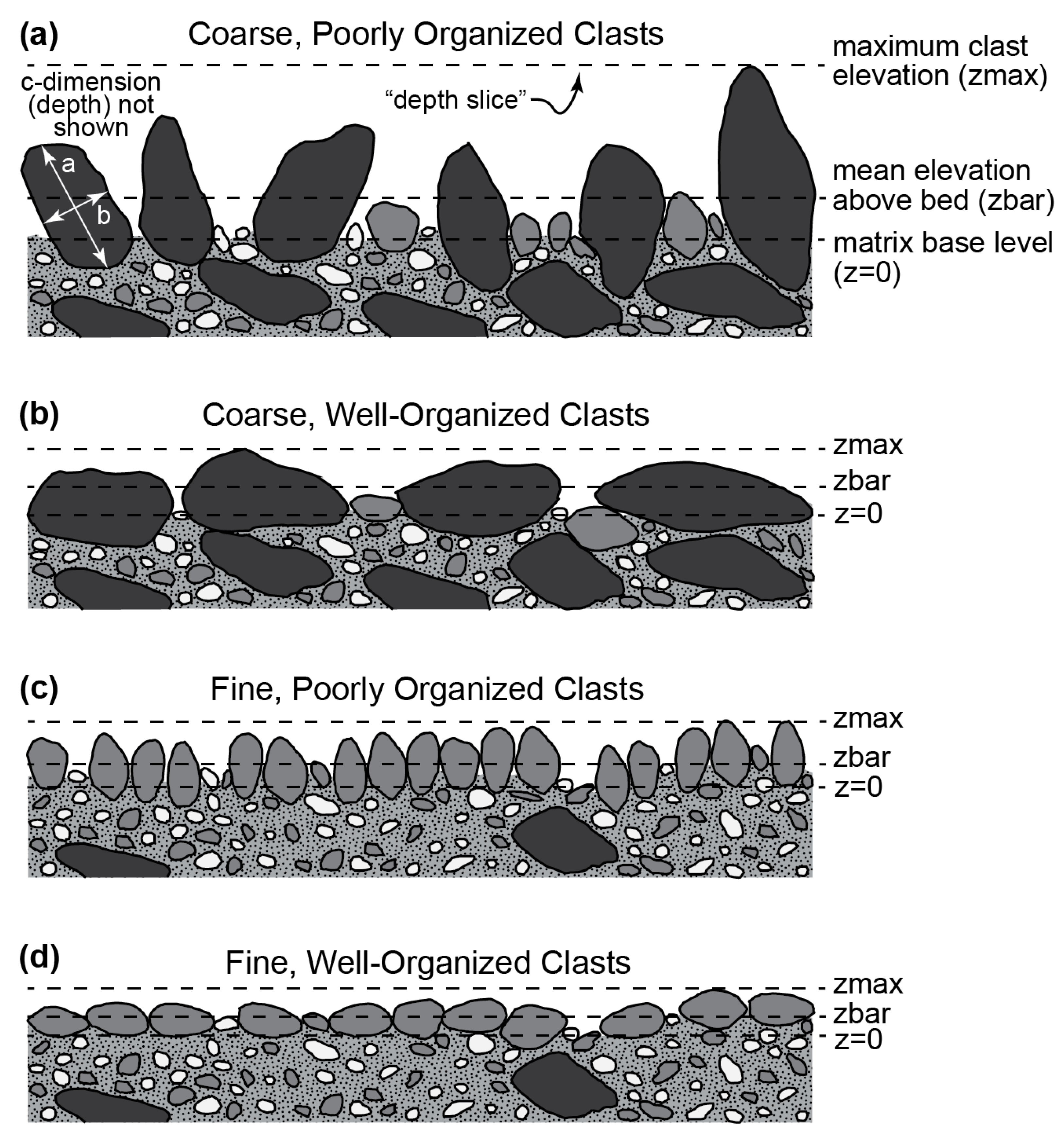
3.1. Conceptual Framework for Quantifying Organization in Heterogenous Gravel Beaches

Surficial gravel armoring and organization can occur in response to both uni and bidirectional currents [19]. Early studies focused on the former, quantifying armoring of mixed gravel beds in laboratory flumes or mountain streams using roughness terms [30], an approach still widely used today [31]. For example, Nikora et al. [19] measured gravel-bed roughness as a random field of vertical measurements (z values) in a three-dimensional space. They determined “roughness” by evaluating the variation of the population of z values (i.e., their standard deviation, σz) in a relatively uniform gravel bed, and evaluated these against the axial dimensions (i.e., a, b, and c axes) of the sampled clasts. However, this approach fails to characterize the three-dimensional nature of surface organization in sediments with variable textures, in which processes such as kinetic sieving produce a surface layer that is generally coarser than underlying deposits [32]. Aberle and Nikora [20] used random field elevation based on laser scanning techniques in laboratory flumes to develop Digital Terrain Models (DTMs) of bed surfaces that describe the structure or roughness of organized gravel sediments on scales ranging from several millimeters to that of the largest clasts within the bed. They found that vertical roughness of gravel beds can be defined by the standard deviations of bed elevations, and that these bed elevations can be used to accurately quantify the development of a coarse surface layer of clasts within that layer. However, this approach is difficult to translate to the field, and does not allow for quantification and comparison of surface clast orientations across a range of clast sizes.
Surficial sediment organization represents the degree to which surface clasts are oriented in their most kinetically stable state. At maximum organization, the long (a) and wide (b) axes of large clasts are parallel to the surface of the bed and the shortest (c) axis is oriented orthogonally to the bed slope. The farther clasts protrude from the surface of the beach matrix, the more likely that those clasts are out of their most stable position; that is, the less organized the surficial sediment. This measure could be characterized by the range of “elevations” above the matrix bed level (z values), quantified as the mean z value (zbar) or—following Nikora et al. [19]—the surface roughness (σz) of a given bed (Table 1). It follows that more highly organized surface sediments would, on average, have lower values of zbar and σz; that is, these would have a lower average elevation above the sedimentary matrix level and less elevation variability (Figure 4). The maximum value of zbar for a sediment plot would be approximately equal to the mean long-axis dimension of clasts within that plot (abar; Table 1) if (1) all large clasts were of similar size (same length of long [‘a’] axes), (2) those large clasts were all positioned with their long axes oriented perpendicularly to the beach slope, and (3) the base of the largest clasts were at the zero-elevation plane. This would represent the minimum theoretical degree of surface clast organization. At sites exhibiting progressively more organization, an increasingly greater percentage of clasts would have their long axis oriented closer to horizontal, and thus be in a more “stable” state.
However, this conceptual framing implies that all clasts are of similar or identical size, both within a plot and across the population of sites being compared. In heterogenous sediments, the range of surface elevations (z values) within a plot may reflect, in part, the range in clast sizes, irrespective of the orientation of those clasts. For example: for two beaches in which all clasts are aligned in their lowest-energy configuration (a and b axes aligned with the plane of the beach slope), the surface rugosity (zbar, or σz) would be greater at the beach with coarser clasts (Figure 4, second panel). This reflects that the c-axis of those coarser clasts is larger—and thus the elevation difference between surface peaks and valleys would be greater—than in a plot with similarly oriented, but overall smaller, clasts (Figure 4, bottom panel). Thus, measures of roughness would depend, in part, on clast size. Moreover, given similar input energy (for example, from breaking waves on a beach), smaller clasts would be expected to be more easily or quickly rotated into a lower-energy, bed-parallel orientation. Thus, within a shoreline reach with consistent hydrodynamic energy, beach sub-sections characterized by finer clasts should become more organized—or organize more rapidly—than those consisting of coarser clasts.
This conceptualization highlights the importance of accounting for clast size in characterizing surficial organization, thereby allowing for meaningful inter-site comparisons regardless of bed clast size. In his analysis of streambeds, Wolman [29] used measurements of the b-axis of individual clasts to characterize the diversity in surficial clast sizes. This axis provides a measurement for large clasts that is analogous to mean grain size (Mz) for the bulk sediment as measured through sieve analysis. In contrast, the level of organization of clasts in a bed is predominantly a function of the orientation of the longest (a) axis of the large clasts: the longer the clasts, the greater maximum surface rugosity in a fully disorganized bed (Figure 4, top panel). We thus consider the average length of the long-axis of clasts in a given plot (abar) to provide the most suitable measure by which to account for clast-size variability.
Following this theoretical framework, we designed a study to quantitatively refine and validate a new organization metric (OM), relying on field measurements of both surface roughness and clast size. In the following section we present this approach, the resulting OM, and validation tests for this new metric.

3.2. Granulometric Analyses

At each site, bulk sediment samples were collected from the side of shallow (<15 cm deep) infaunal excavation by inserting a 15-cm long, 10-cm diameter core sampler horizontally into the undisturbed sediment of the excavation wall. Samples collected in this manner provide a representative profile of grain size in three 5-cm deep horizons, i.e., upper, middle, and lower strata. Care was taken to include all coarse clasts that could fit into the core sampler. Where present, clasts with b-axes ≥10 cm were excluded due to size limitations of the core sampler.
Coarse fractions (>4 phi [φ] [0.0625 mm]) were dry sieved at 1-φ intervals following procedures of Folk and Ward [33]. Fine fractions separated by wet sieving were analyzed using a Beckman Coulter LS 13320 Laser Diffraction Particle Size Analyzer to 11φ (0.00049 mm; fine clay). Grain-size statistics were calculated following Folk and Ward [33] using the logarithmic (inclusive) graphical method.

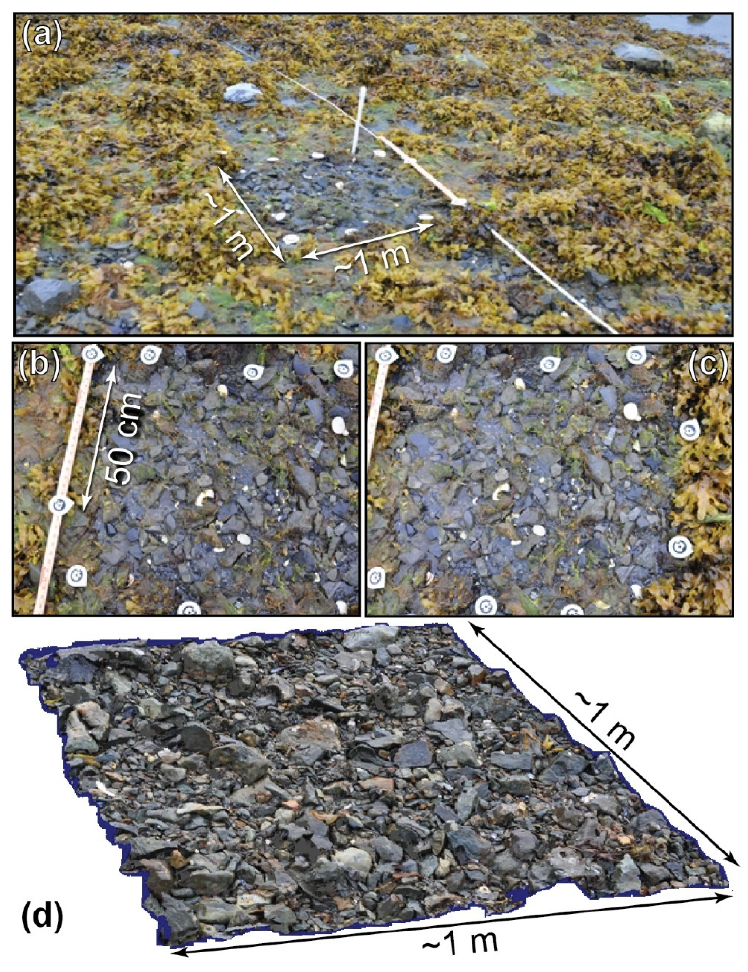
3.3. Field Geomorphology and Photogrammetry

General morphological characteristics, including overall beach slope, sediment composition, and fetch exposure were qualitatively described for each study site. At each, plots, roughly square and ~1 m2 in area, were marked out using a series of 10-cm diameter coded targets (Figure 5). The surface of each plot was cleared of all plant cover and large motile invertebrates. Care was taken to ensure that clasts within these plots remained undisturbed during the clearing process. Vegetation was cut from the individual clasts, exposing the surface of the clasts such that morphological analysis captured the shape and form of the bare clasts (Figure 5b,c). Lateral reference scales within each plot were provided by a coded meter stick placed on the beach surface (Figure 5b). Vertical reference was provided by a PVC pipe oriented with a hand level (Figure 5a).
A series of high-resolution stereophotograph pairs was taken of each plot (e.g., Figure 5) using a Nikon D90 camera with a 20.0-mm lens specially calibrated for working with the PhotoModeler ScannerTM (EOS® Systems Inc., Vancouver, BC) software package. Paired photos were offset laterally by <50 cm. These pairs were taken from at least two angles and elevations from each side of a given plot to ensure all visible surfaces of each clast were photographed. This provided stereophoto pairs from a variety of orientations (Figure 5b,c). A series of 5–10 stereo pairs was collected from each plot. Generally, plots dominated by coarser-grained gravel required a greater number of photos than those with finer clasts due to the number of orientations needed to capture the three-dimensional morphology of larger cobbles and boulders.
Following the collection of the photographs, Wolman Pebble Counts [32] were conducted for each plot in order to determine the long (a), intermediate (b), and short (c) axes for the largest 15–47 surface clasts within each plot. The range in the number of clasts measured reflects the diversity in clast size within a given plot. Those with larger and more diverse clast sizes required additional clast counts to characterize clast diversity within the plot. These were averaged for each plot and are given as abar, bbar, and cbar, respectively.
Finally, in an experiment designed as a validation test for the method and the organization metric, the surface of four randomly selected plots was manually disturbed following completion of pebble counts. Clasts comprising the surface armor were vigorously disturbed with an entrenching tool, shovel, or trowel. The photo plots were then re-photographed and analyzed in the same manner as for the initial, undisturbed plots.

3.4. Processing and Analysis of Photogrammetric Data

Stereo-photo pairs were analyzed using PhotoModeler ScannerTM. This system produces a dense point cloud from photographs of textured surfaces (surface sediment plots, in this case). Photos were inputted into the software package and stereopairs identified. Coded targets, visible on all plot photos, were manually identified on each photo and cross-referenced between photos. Photos were then “idealized” to account for artifacts associated with the curvature of the camera lens. The resulting photos were edge-warped such that each photo captured a true projection of space, without lens distortion and with square pixels and a centered principal point. Photo scale and orientations were calibrated using the meter stick and the vertical pipe.
Three-dimensional maps of plots were created at ~1-mm horizontal resolution (Figure 5d) and trimmed to the given plot areas using coded targets as plot area boundaries. Each point within a plot is assigned an x, y coordinate in non-referenced space, and an elevation value (z) above an artificial horizontal plane. The number of coordinate points obtained from a given 1-m2 photoplot ranged from ~250,000 to ~700,000. This variability reflects differences in the area covered by the photoplots and the complexity of the surficial fabric formed by the clasts. The resulting point mesh data were exported as digital terrain models (DTMs) into MATLAB for comparative analyses. All data underwent first-order detrending to remove the slope within the data set that resulted from the natural slope of the beach. The resulting z values were corrected such that the minimum elevation point in a given plot was assigned a value of 0 mm. Surface elevation (z-axis) statistics such as maximum, minimum, mean (zbar), median, and standard deviation (σz) elevations were calculated for each plot. Horizontal slices were then taken through the DTMs at 5-mm increments, at the median elevation, and at elevations representing the 10th and 25th percentiles above the minimum elevation in a given plot. The percent of data points above and below each of those slices was then calculated.
Combined with our Wolman Pebble Counts and surface sediment grain-size analysis, these data provide variables that were used to characterize size, and surficial organization of sediments within each plot.

3.5. Inferential Statistics

Site comparisons used for validation and testing of our approach were evaluated using resampling techniques for comparison of means, analysis of variance (ANOVA), and regression analyses. These were calculated using a Microsoft Excel add-in developed by Resampling Stats [35]. Two-factor ANOVA was calculated using the StatPlus add-in to Excel. Where particular differences were expected based on field observations, 1-tailed tests were used.
For comparing regression slopes, the paired linear regression approach outlined in Zar [36], was implemented with IGOR Pro version 6.22A (http://www.wavemetrics.com; accessed on 9 March 2022). This statistic compares both the slope of two regressions and the mean y-values of the data comprising two regressions. First, it assesses whether rates of change for the slopes of two regressions are the same. Next, it compares the “statistical elevations” of two populations (as distinct from z-values in the photogrammetric analyses) to assess whether they are the same. A significant difference in either comparison indicates that the populations of values are statistically different.
Finally, given the heterogeneity of PWS lower intertidal beaches in terms of lithology and wave exposure (particularly in comparison to conditions experienced in laboratory settings), and to minimize false negatives, we adopted an α value of 0.1 as the critical level of significance for all statistical testing. Values of “p” between 0.1 and 0.2 are considered to represent trends. Standard deviation (SD) is used to represented degree of variability for individual measurements (e.g., OM) and standard error (SE) is used where variables are means (e.g., zbar or abar).

4. Results

4.1. Field and Laboratory Results

Treatment status, nominal tidal elevation, mean clast length (abar) calculated from Wolman Pebble Counts, and photoplot data (elevation standard deviation (σz), and the calculated values for our organization metric (OM)) are presented in Table 2. Mean particle size (Mz) and % cobble/pebble/granule (gravel) from grain-size analyses of bulk-sediment samples from the upper sediment horizon at each site, as well as its nominal tidal elevation, are presented in Supplemental Table S1.
Sediment textures varied considerably among sites. The mean grain size (Mz) of the upper 5 cm of sediment for all 37 sites surveyed ranged from 3.01 to 51.85 mm and averaged 14.7 ± 10.3 mm (Supplemental Table S1). These values reflect the presence of a very wide range of particle size classes in the sediments among the sites, i.e., clay to small cobble. Percent gravel averaged 75.3% ± 16.3 and ranged from 32.1 to 99.9%.
Among surficial clasts in each plot, the subset of the largest clasts measured through Wolman Pebble Counts had a mean long-axis dimension (abar) of 4.8 to 19.3 cm, averaging 9.19 ± 0.41 cm across all sites (Table 2). Calculated abar and Mz values were not correlated (p > 0.5; resampling linear regression), indicating that the length of surficial clasts was not related to the composition of the underlying whole sediments.
We found that both Mz and percent gravel were highest in the upper stratigraphic horizon and were lower in the middle and lower horizons (Table 3). Sand content was highest at the middle horizon. Silt/clay content was lowest at the upper level and highest in the lower horizon. The differences between the horizons were significant for all variables except the percentage of silt/clay.
The mean surface elevation of sediments in our slope-corrected photoplots (zbar) was, on average, 4.51 ± 0.25 cm above the artificial horizontal plane at the lowest imaged elevation (z = 0; see Figure 2). This value is ~50% of mean measured abar for these sites. The standard deviation of these photoplot elevations (σz) averaged 1.51 ± 0.11 cm and ranged from 0.52 to 6.09 cm. As expected, both zbar and σz exhibited very strong correlations with abar values (Figure 6): The correlation of σz to abar (p << 0.0001; resampling linear regression) was stronger than that for zbar (p = 0.0001) and thus provides a stronger statistic with which to evaluate clast organization. However, σz is not clast-size independent, as it exhibits a very strong relationship with abar (Figure 6). Thus, as anticipated, σz is not suitable by itself for describing organization among sites with varying clast sizes.

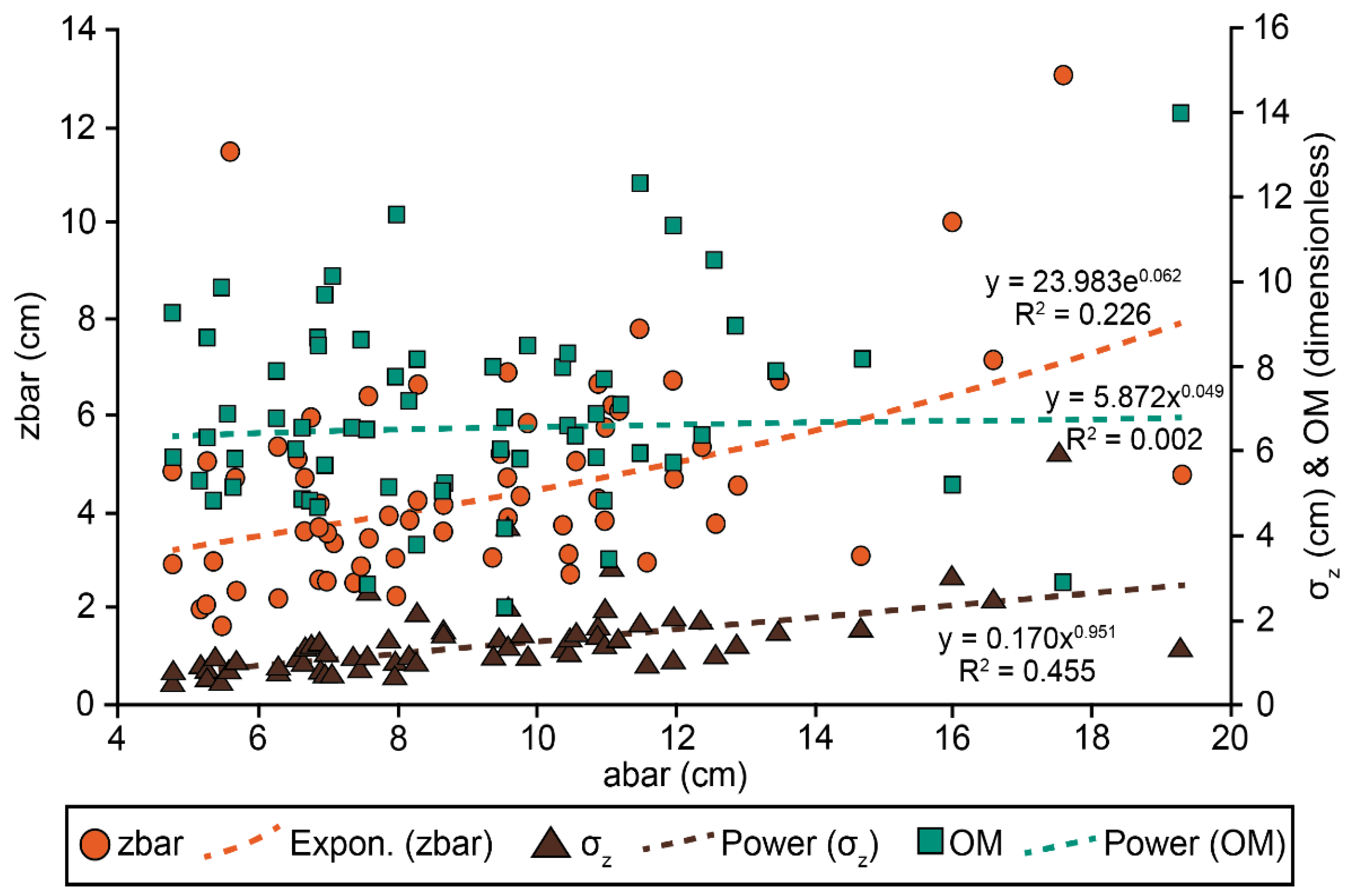
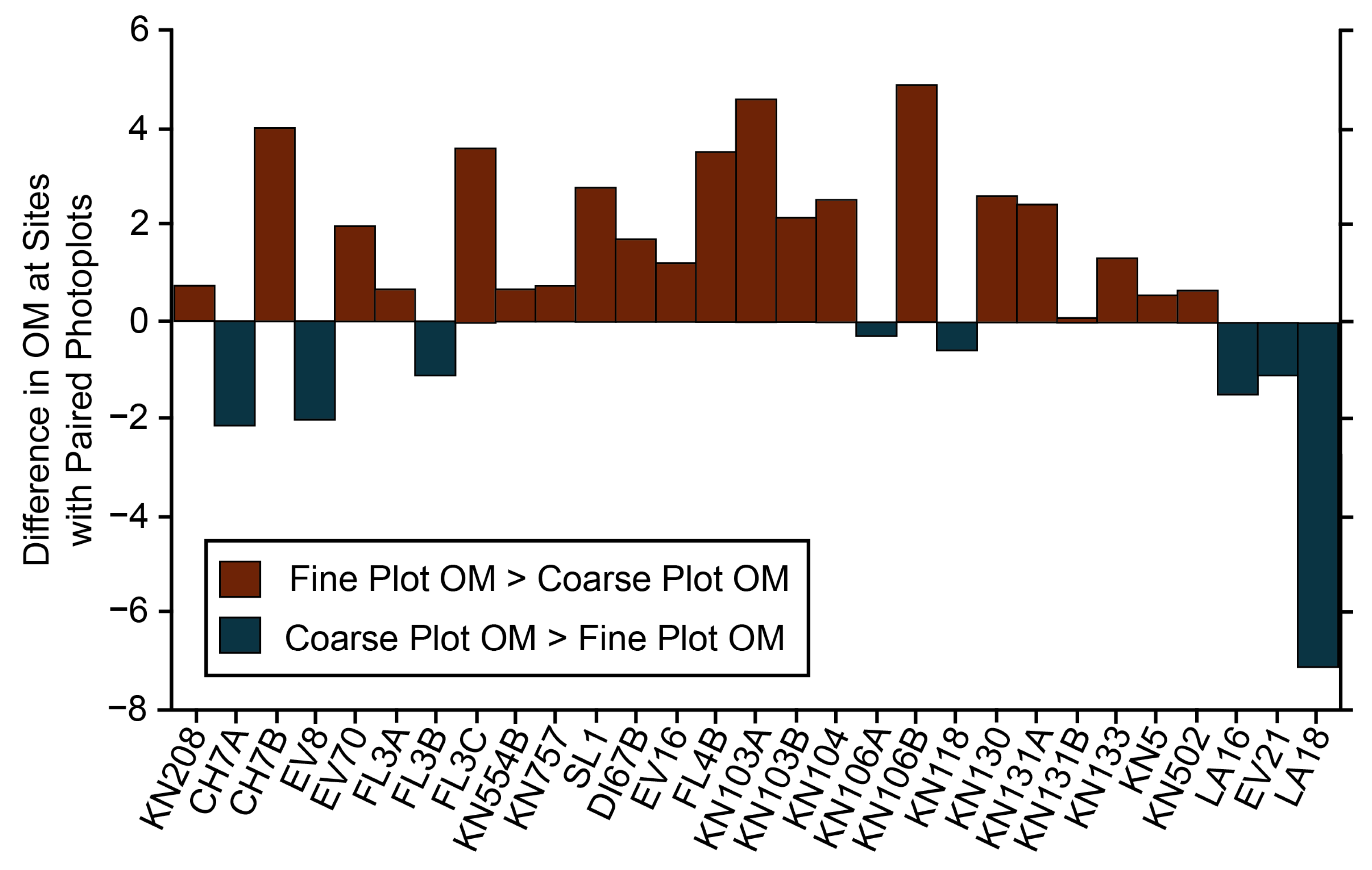
4.2. Derivation of the Organization Metric

Given the myriad clast sizes observed on PWS beaches, and the range in the degree of organization of those clasts in the lower intertidal zone, variability in elevations (z) within a plot can be large. We found a significantly stronger correlation between clast size (abar) and the range of elevations present in a given plot (i.e., σz; where r = 0.67, p = << 0.0001; Figure 6) than between abar and the average plot elevation (zbar; where r = 0.48, p = 0.0001; resampling regression). This analysis confirms our theoretical framework for applying a measure of surface roughness (as characterized by σz) in our organization metric and normalizing by the clast-size measure to which organization is most sensitive (abar).
Following these considerations, we derive the following formula for calculating our dimensionless organization metric (OM):
OM = abar/σz,
in which both abar and σz values are given in cm, so that higher values represent higher degrees of surficial organization (clasts situated in most stable orientations).
The calculated OM values for all sites ranged from 2.27 to 14.06 (Table 2; Figure 6), with a mean value of 6.89 ± 2.307. The OM values are independent of abar (p = 0.25). Thus, equal values of OM should indicate that the mean orientation (flatness) of the clasts relative to beach angle is similar at sites at which clast lengths differ substantially.

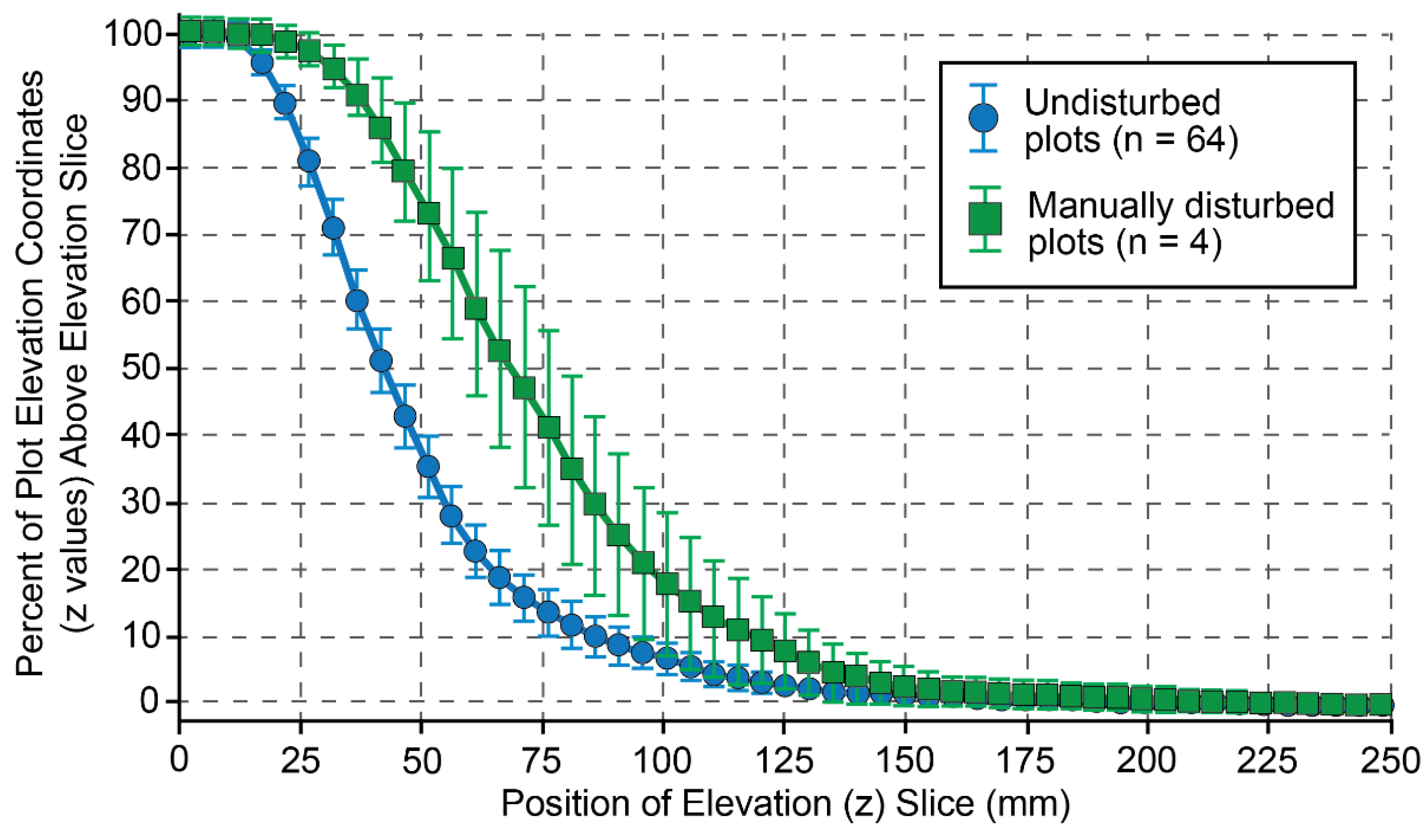
4.3. Validation of the Organization Metric

We employed three independent tests to evaluate the OM function. Together, these demonstrate that differences in the OM values accurately reflect differences in surficial clast organization.
The first test relies on the fact that, all other factors being equal, the distribution of z-values (the “elevation” at each x,y point in the DTMs) is itself an indicator of the degree of organization, as demonstrated by Aberle and Nikora [20]. In Figure 7, we present the mean percentage of z-values extending varying distances above the standardized z = 0 matrix bed elevation for a given DTM for all undisturbed plots and four disturbed plots surveyed (KN5-1, KN5-2, KN208-1, and KN208-2). Thus, at the 50-mm slice, 35% of the z-values for the undisturbed plots extend above the standardized zero elevation whereas nearly 73% of the z values for the four disturbed plots extend above that elevation, indicating a greater degree of disorientation in the clasts in the disturbed plots. This analysis demonstrates that a larger proportion of the z-values forming the surfaces of the DTM for the undisturbed plots occurred significantly closer to the standardized base level (zero on the x-axis) than in the disturbed plots (p << 0.0001; resampling comparison of means).
The second test involved an assumption that smaller clasts are more easily rotated into a flattened position because less hydrodynamic (wave or flow) energy is required to move them. Thus, assuming that seasonally averaged wave energy along a given short stretch of beach distal from headlands (<50 m) is approximately equal, areas of that beach with finer clasts (smaller abar) should be more organized than those characterized by coarser clasts (larger abar). It follows that OM values for the plot with finer clasts should, on average, be higher (more apparently well organized) than the one with coarser clasts. The predominance of this pattern is clear (Figure 8). At these sites, plots with smaller clasts had higher values of OM (were more organized) at 21 of 29 sites. Mean OM for plots with smaller clasts (7.3 ± 0.4) was significantly greater than that observed for plots with larger clasts (6.3 ± 0.5; Table 4; p = 0.080; paired 1-tailed resampling comparison of means).
Our third field functionality test for OM compared pre and post-disturbance values for OM and σz for four plots that were manually disturbed with a shovel following the initial photo-documentation. We predicted that OM in the artificially disturbed plots would be lower than in those same plots prior to manual disturbance. Indeed, following disturbance, zbar increased 79% ± 51% (p < 0.0001; paired 1-tailed resampling comparison of means; mean σz also increased (52.0% ± 40.0%; p < 0.0001; Table 5) and mean OM decreased significantly (31.1% ± 8.7%; p < 0.0001; Figure 9). All three variables responded significantly to disturbance.

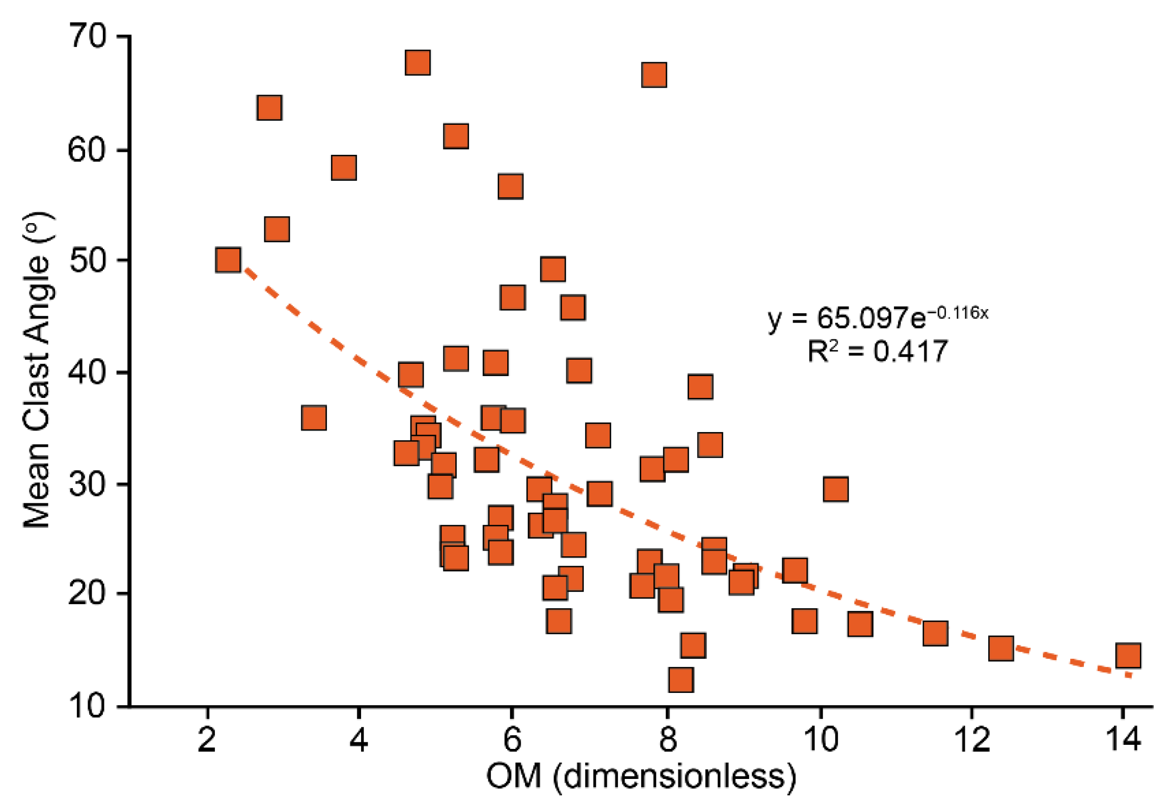
4.4. Relationship between OM and Clast Angle

The conceptual framework for OM suggests that the mean orientation of the long (a) axis of armoring clasts with the plane of the beach (the “clast angle”) should decline as OM increases, i.e., the clasts become more parallel with the surface of the sediment. We calculated the average clast orientation in each photoplot by designating abar as the adjacent side of a right triangle and zbar as the opposite side. The tangent of the ratio of these sides (zbar/abar), was used to approximate the average angle formed by the armoring clasts with the surface of the beach. The resulting comparison between OM and mean clast angle, shown in Figure 10, indicates that, indeed, mean photoplot clast angle decreases at higher values of OM, and that the relationship is highly significant (p<<0.0001; resampling regression).

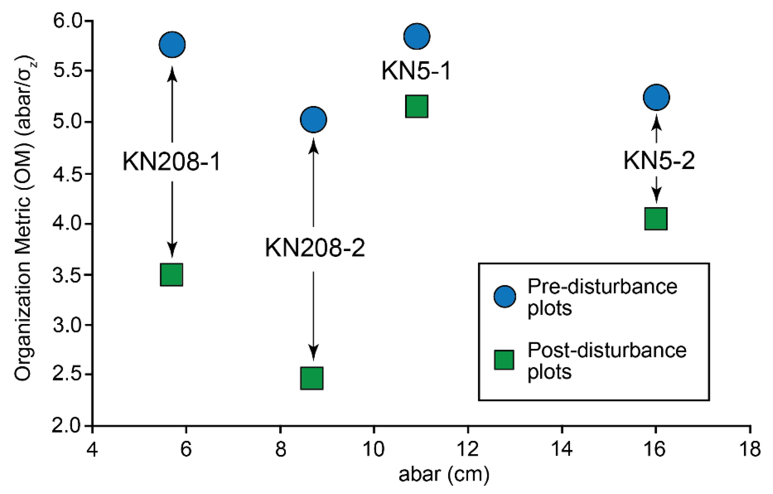
5. Case Study: Use of OM to Quantify the Long-Term Impact of Beach Washing

The question arises: “How can an organization metric be used?” To demonstrate, we present the outcomes of a case study using our new OM to explore the long-term (21 years) effects of post-spill cleanup efforts on PWS beaches. Specifically, we compared the degree of surficial clast organization in the lower intertidal zone of beaches which were left untouched following the EVOS with those that likely experienced significant physical disturbance caused by HP/HW washing (designations of our sites shown in Figure 3 and given in Table 2). In addition to demonstrating the efficacy of our approach and OM, a goal of this case study is to assess whether those beaches which underwent HP/HW washing following the EVOS would be less organized than those of unwashed beaches. The likelihood of differing degrees of clast organization associated with post-spill treatment was first proposed by Lees and Driskell [18], who concluded that large sedentary megafauna, especially adult and sub-adult hard-shelled clams, were significantly less abundant in washed beaches. They suggested that reduced organization would affect the rate of recovery of assemblages that were rich in the areas prior to the EVOS cleanup. Comparing beach sedimentology below the surface through our depth-profile samples, we were further able to test washing effects extended deeper into the sediment than just disturbance of surficial armor.
Mearns reports that only 89% of the PWS shoreline segments oiled during the EVOS were treated in some manner [37]. Of these, he reported that a large fraction (ca. 79%) was treated to remove oil with approaches such as HP-HW washing, which are very disruptive to surficial stratigraphy and organization (e.g., Figure 4). Unfortunately, records from the post-spill clean-up period are incomplete and do not allow for identification of all beaches or beach segments that were treated with such washing. As such, we specifically selected beaches and beach segments that had been personally observed to have undergone this treatment during the clean-up period (“observed washed”; DCL) or were highly likely to have undergone this treatment (“presumed washed”) based on interrelationships between location, degree of oiling, and governmental agency records [28,38]. We group these as “presumed” washed sites. For analyses in the following section, we have grouped the latter two categories and refer to them as O/P washed sites.
Given uncertainty regarding post-EVOS treatments, we applied a ‘weight-of-evidence’ argument to the outcomes of our analyses for those sites classified as “O/P washed”, in order to improve confidence in this designation. One can expect HP/HW washing to alter a variety of sedimentary and stratification characteristics, beyond the hypothesized impact on surficial organization. For example, for beaches that underwent HP/HW washing, we would expect to see predictable relationships, on average (Table 6):
  • Mz in surficial sediments at unwashed sites should be finer than at O/P washed sites because flushing associated with HP/HW washing would have removed much of the fine fraction.
  • The proportion of gravel/cobble therefore should be greater, and the proportion of finer sediments would be lesser, than at unwashed sites.
  • Mz in the surficial 5-cm horizon should be coarser than in deeper horizons due to that same flushing of fine sediments; and
  • The proportion of silt/clay should be lower at all horizons at O/P washed sites than at unwashed sites.
We would also expect to see predictable relationships in abar and the photogrammetric values, on average (Table 7):
5.
Because washing should not affect the large clasts, abar should be similar.
6.
zbar and σz should be greater than at unwashed sites.
7.
OM should be lower than at unwashed sites.
Weight-of-evidence in these tables argues strongly that, on average, the two treatment categories are distinctly different, i.e., one group of sites was unwashed, and the other group was washed. Mz, which responds to loss of sand and silt/clay due to washing, differed significantly between unwashed (9.00 ± 0.95 mm) and O/P washed sites (18.21 ± 2.40 mm; p-0.0076, resampling comparison of means; Table 6). Gravel was greater at O/P washed sites (83.0% ± 2.4 vs. 73.9 ± 2.3; p = 0.004) because a large volume of sand and silt/clay that was washed away. Moreover, Mz in the lower horizon was significantly lower than in the upper horizons (p-0.014; 2-tailed resampling ANOVA). Finally, % silt/clay was significantly lower in upper and lower horizons than at O/P washed sites (p << 0.0001 and p = 0.08, respectively) because it had been flushed out by washing.
Notably, differences in abar between unwashed and O/P washed sites were not significant (p = 0.94; Table 7). This was predictable because large clasts likely would not be added or removed from an area by washing. It was unexpected that zbar was not significantly higher at O/P washed sites (p = 0.22). However, σz was significantly higher at O/P washed sites (p = 0.073) and OM was significantly higher sites at unwashed sites, as predicted above (p = 0.06).
Comparison of OM values for unwashed and O/P washed sites (Figure 11) reveals overall substantially lower degree of organization and considerably more variability in OM in the O/P washed sites. Slopes and separation on the y-axes (statistical elevations) of the OM regressions for the unwashed and O/P washed sites were compared using the paired linear regression approach (Figure 11). The data clouds overlap considerably, reflecting the great variability in environmental conditions at these sites. Nevertheless, the slopes are not statistically different (p > 0.5; paired linear regression as calculated by IGOR), again demonstrating that OM fits a primary criterion for metric suitability (clast-size independence). However, despite the high variability among the sites, the statistical elevations are statistically different (p = 0.025), with the OM regression for unwashed sites significantly higher than for O/P washed sites. However, both are relatively weak, as indicated by the relatively low p-values for the regressions (p > 0.63 and p > 0.34, respectively). This indicates that beach washing reduced armor clast organization at O/P washed sites and this effect persisted 21 years after the cleanup.
In Figure 12, we present the mean percentage of z-values extending varying distances above the standardized z = 0 (see Figure 2) elevation for a given sets of DTMs for all unwashed, O/P washed surveyed, and four plots manually disturbed during the study (KN5-1, KN5-2, KN208-1, and KN208-2). At the 50-mm slice, 31% of the z-values for the unwashed plots extend above the standardized zero elevation, compared to nearly 37% of the z-values for O/P washed plots. Finally, 73% of the z-values for the four disturbed plots extend above that elevation. This pattern continues for the remainder of the O/P washed and disturbed curves. This analysis demonstrates that a larger proportion of the z-values forming the surfaces of the DTM for the undisturbed plots occur significantly closer to the standardized base level (zero on the x-axis) than both the O/P washed and manually disturbed plots. However, if we assume that O/P washed sites were disturbed through HP/HW washing to a degree similar to our manual disturbance, this also suggested that these plots have recovered substantially since they were initially disturbed by the beach cleanup in 1989 and 1990.

6. Discussion

6.1. Utility of an Improved Organization Metric

In its most simplistic form, cross-shore swash zone sediment transport is a function of the shear stress of wave swash and backwash over the bed and the critical shear stresses required to initiate movement of clasts. Once an armor has developed within coarse, surficial sediments, a stronger current is required to transport individual clasts, a phenomenon termed “structural strengthening” [12]. Organization of this armor layer further enhances the stability of the bed by maximizing clast-on-clast contacts, increasing the shear stress required to initiate movement of any one clast. Factors such as clast size, clast pivotability (relative projection of a clast above the bed, influenced by clast shape and orientation relative to surrounding clasts), degree of imbrication, and presence of a stable coarse-grained armor can alter this critical shear stress [5,6]. The protrusion of clasts above the matrix bed level (increased pivotability) increases friction coefficients, thereby making the bed more erodible, whereas the most stable bed configuration is one fully armored, that is, one that has a high friction angle and low height above the bed where the flow is acting [39]. Thus, an armored bed that is organized is in a highly stable configuration.
Our newly proposed metric for quantifying organization builds upon a wealth of work to quantify gravel bed structure or “roughness” in fluvial systems, including those that apply similar digital mapping techniques [40,41,42]. However, in the wave-exposed (bi or multi-directional flow) gravel beach system, the consequences of exposure to water flow are quite different from what is reported in unidirectional flow streams or flumes. Notably, in the latter, exposure to downstream currents increases, rather than decreases, roughness [43]. Our approach is statistically robust, fast and easy to implement in field settings, and—because resulting OM values are independent of sediment grain size—appropriate for use across a wide assortment of gravel beaches characterized by clasts of widely varying sizes and shapes, and overall sediment compositions ranging from well-sorted to heterogeneous. As the case study shows, this approach can be employed on disparate intertidal heterogeneous gravel beaches that are subject to any manner of natural or anthropogenic disturbance. Further, OM serves as a proxy for surface clast stability in addition to clast orientation/angle. For example, a plot with partially buried clasts (and thus more muted plot microtopography; lower zbar and σz values) would have a higher resulting value for OM than a plot with clasts of identical size and orientation, but in which those clasts sit entirely upon the surface of the bed matrix. This is likely one factor that accounts for the wide variation of OM at any specific value for abar (Figure 11). Likewise, OM values would be higher in sites with high degrees of imbrication, as the overlapping clasts themselves create the visible bed surface, minimizing microtopography above the z = 0 surface. The development of imbrication reflects extrinsic factors such as wave energy, as well as characteristics of the clasts themselves, such as clast shape: flatter clasts are more easily imbricated than clasts in which the c-axis approaches the dimension of the b- and a-axes. Because OM is normalized only by clast a-axes, it is insensitive to clast shape. However, imbrication is conspicuously absent from most PWS beaches [5] and was not observed in any of our study sites and cannot be addressed with these data. Thus, the response of OM to different degrees of imbrication remains an avenue for future exploration.
The newly developed OM uses an off-the-shelf digital camera which, even combined with a proprietary software license and peripherals (estimated at <US$5000 total in 2021), cost far less than traditional ground-based LiDAR (3D laser scanner) systems. However, it would be difficult to adapt this system to subtidal or in-stream environments. Such applications would be particularly useful, for example, in assessing the effects of marine aggregate harvesting [44] or scallop dredging [45] on clast organization in heterogeneous gravel beds, which have been found to host rich sedentary megafaunal assemblages [45,46,47]. Because it is likely that clast organization is an important component in the recovery of disturbed megafaunal assemblages in coarse sediments [18], such knowledge would help in estimating the likely time required for recovery of the valuable targeted or untargeted living resources that are “harvested” during these operations. Recovery time is an important element in weighing the overall environmental cost/benefit of a proposed activity that is generally severely underestimated [18,48,49].
It is likely that newer technologies such as handheld (or now even phone-based) LiDAR and structure-from-motion could provide efficient alternatives to the PhotoModeler approach presented here. These have been demonstrated for use in similar-sized plots (e.g., [50,51,52], and at least the former could be applied in shallow-water environments. Further, expanding our approach with digital, in-situ grain-size analysis [53] would improve reliability of clast measurements used in OM for grain-size normalization (abar), and remove potential biases associated with Wolman Pebble Counts (e.g., [54]. However, care must be taken to ensure that clast-size measurements using such an approach are accurate and comprehensive. For example, in a case in which clasts are in a disorganized state (oriented on end, with ‘a’-axes perpendicular to the beach slope), in-situ size measurements would be unable to capture the full length of the a-axes, as a substantial percentage of the length of the clast could be buried and not visible from the surface photogrammetrically, resulting in inaccurate values for abar.

6.2. New Insights into Sedimentologic Structure of Heterogenous Gravel Beaches in Prince William Sound

Our comparison of unwashed and O/P washed beaches in PWS reveals new insights into the long-term effects of HP/HW washing in both surficial clast organization and shallow subsurface stratigraphy.
Overall, PWS beaches are coarser grained than heterogenous coarse beaches described elsewhere. For example, we found that gravel comprised 32% to nearly 100% (mean: ~75%) of surficial sediments, as compared with only 15–24% reported by Hayes et al. [2] for Prince William Sound beaches, Jennings and Shulmeister [3] in New Zealand, and Mason and Coates [4] from a literature review. At unwashed sites, we found that both Mz and percent gravel were higher in the upper and middle horizons and were lowest in the lower horizon (Table 5). Sand content was highest in the upper horizon. Silt/clay content was lowest in the middle level and highest in the lower horizon. None of these differences were significant. This is in contrast to observations of gravel stratification in beaches elsewhere, such as Wales [55] and Argentina [6]. A possible reason for this is that PWS beaches are geologically quite ‘young’, i.e., they were only established within the intertidal zone during the 1964 Great Alaska Earthquake, which elevated or lowered beaches considerably in western PWS [25,56]. However, differences between unwashed and O/P washed beaches—in which the O/P washed beaches were significantly overall coarser and, at least within the upper and lower horizons, more gravel-dominated than unwashed beaches—importantly reveals that HP/HW beach washing altered the vertical structure of these PWS beaches down to at least 15 cm.
Calculated values of OM were statistically independent of the broad range of grain sizes across our 37 sampled beaches in PWS, but the OM values were quite variable. This reflects the complexity of processes responsible for development of surficial organization in heterogeneous gravel sediments in the lower intertidal zone. For example, the responsiveness of clasts on a beach to reorientation into a more stable state (i.e., their pivotability) could be influenced by clast geologic composition (e.g., shape and specific density), differences in wave exposure or tidal currents), or the susceptibility of those clasts to reworking, as influenced by biological activity (e.g., cover of clasts by heavy algal cover, mussels, or barnacles, and excavation activities of predators). For example, the potential role of tidal forcing is suggested at IN32, which had the highest observed OM (13.99). This site is located in a narrow channel protected from wave action, but exposed to strong, twice-daily, bidirectional tidal currents. Unfortunately, our small sample size of beaches unaffected by post-EVOS cleaning activities prohibits exploration of the role of these factors in sediment organization. This remains an opportunity for future studies and modeling efforts.

7. Conclusions

Using western Prince William Sound (PWS), Alaska (USA) as a natural laboratory, we developed a new metric for quantifying the degree of organization of large clasts in surficial sediments in coarse, heterogenous beaches. This unique approach employs creation of three-dimensional digital terrain models from small study plots in the lower intertidal zone on a diverse series of heterogeneous gravel beaches in PWS. The resulting organization metric (OM) is independent of differences in clast size. Values varied widely among the beaches sampled, but OM is a useful tool for quantifying an important aspect of the organization on armored beaches.
Overall, this study developed and field-tested a new approach for quantifying organization of heterogenous coarse sediments in diverse, terrestrial settings, including deserts. Although our particular approach relies on quantification of surface texture from photogrammetric analyses and field measurements of clast sizes, newer tools such as ground-based LiDAR and structure-from-motion could allow for faster application and more accurate measures of surface texture through digitized grain-size analysis.
Finally, our case study using this new metric found that organization of the armored layer on beaches was significantly lower on those beaches which were observed or presumed to have been washed following the oil spill in PWS than on those which were left unwashed. Combined with observations of relatively coarser and more gravel-dominated stratigraphy to a depth of at least 15 cm in these washed beaches, this reveals that the physical structure and sedimentology of beaches that underwent post-spill washing remained significantly altered 21 years after the cleanup. This finding has important implications for beach management during and following major disturbance events (e.g., cleaning or dredging).

Supplementary Materials

The following supporting information can be downloaded at: https://www.mdpi.com/article/10.3390/jmse10040525/s1. Table S1: Results of Granulometric Analysis.

Author Contributions

Conceptualization, D.C.L.; methodology, D.C.L., C.J.H. and D.M.F.; laboratory analysis, C.J.H.; data analysis and statistics, D.C.L.; investigation and resources, D.C.L.; writing—original draft preparation, D.C.L.; writing—review and editing, C.J.H., D.M.F. and D.C.L.; visualization, D.C.L. and C.J.H.; funding acquisition and project administration, D.C.L. All authors have read and agreed to the published version of the manuscript.

Funding

This research was funded by the NOAA/NMFS Exxon Valdez Oil Spill Office for the Exxon Valdez Oil Spill Trustee Council under Contract No. AB133F-10-CQ-0066 from Western Acquisition Division Contracts Branch to Littoral Ecological & Environmental Services.

Institutional Review Board Statement

Not applicable.

Informed Consent Statement

Not applicable.

Data Availability Statement

All supporting data for this study are reported in the manuscript and/or supplemental materials. Raw data for sediments and photogrammetric analyses can be obtained from D.C.L. or C.J.H.

Acknowledgments

This is contribution 4088 of the Virginia Institute of Marine Science, William & Mary. The authors thank David and Annette Janka, operators of the R/V Auklet, and Terry Kennedy, Alaskan Wilderness Air, for valuable logistical assistance in data collection. Marcio Boechat Albernaz provided critical assistance in the field and conducted granulometric and statistical analyses for the bulk sediment samples in the laboratory. Emily Hein designed and ran MATLAB codes for analyzing photogrammetric data. We are also grateful to Matt Klymson and Dan Money of EOS® Systems (Toronto, ON, Canada) for assisting us in adapting the PhotoModeler Scanner system to our concept for measuring organization of heterogeneous sediment.

Conflicts of Interest

The authors declare no conflict of interest. The funders had no role in the design of the study; in the collection, analyses, or interpretation of data; in the writing of the manuscript, or in the decision to publish the results.

References

  1. Wentworth, C.K.A. A scale of grade and class terms of clastic sediments. J. Geol. 1922, 30, 377–392. [Google Scholar] [CrossRef]
  2. Hayes, M.O.; Michel, J.; Noe, D.C. Factors controlling initial deposition and long-term fate of spilled oil on gravel beaches. In Proceedings of the International Oil Spill Conference, San Diego, CA, USA, 1 March 1991; American Petroleum Institute, Allen Press: Lawrence, Kanas, 1991; Volume 1991, pp. 453–460. [Google Scholar] [CrossRef]
  3. Jennings, R.; Shulmeister, J. A field based classification scheme for gravel beaches. Mar. Geol. 2002, 186, 211–228. [Google Scholar] [CrossRef]
  4. Mason, T.; Coates, T.T. Sediment transport processes on mixed beaches: A review for shoreline management. J. Coast. Res. 2001, 17, 645–657. Available online: https://www.jstor.org/stable/4300216 (accessed on 7 April 2022).
  5. Hayes, M.O.; Michel, J.; Betenbaugh, D.V. The intermittently exposed, coarse-grained gravel beaches of Prince William Sound, Alaska: Comparison with open-ocean gravel beaches. J. Coast. Res. 2010, 26, 4–30. [Google Scholar] [CrossRef]
  6. Isla, F.I. Overpassing and armouring phenomena on gravel beaches. Mar. Geol. 1993, 110, 369–376. [Google Scholar] [CrossRef]
  7. Kirk, R.M. Mixed sand and gravel beaches: Morphology, processes and sediments. Prog. Phys. Geogr. 1980, 4, 189–210. [Google Scholar] [CrossRef]
  8. Horn, D.P.; Walton, S.M. Spatial and temporal variations of sediment size on a mixed sand and gravel beach. Sediment. Geol. 2007, 202, 509–528. [Google Scholar] [CrossRef]
  9. Van Wellen, E.; Chadwick, A.J.; Mason, T. A review and assessment of longshore sediment transport equations for coarse-grained beaches. Coast. Eng. 2000, 40, 243–275. [Google Scholar] [CrossRef]
  10. Hein, C.J.; FitzGerald, D.M.; Buynevich, I.V.; Van Heteren, S.; Kelley, J.T. Evolution of paraglacial coasts in response to changes in fluvial sediment supply. Geol. Soc. Lond. Spec. Publ. 2014, 388, 247–280. [Google Scholar] [CrossRef]
  11. Carter, R.W.; Rihan, C.L. Shell and pebble pavements on beaches: Examples from the north coast of Ireland. Catena 1978, 5, 365–374. [Google Scholar] [CrossRef]
  12. White, W.R.; Day, T.J. Transport of graded gravel bed material. In Gravel-Bed Rivers: Fluvial Processes, Engineering and Management; Hey, R.D., Bathurst, J.C., Thorne, C.R., Eds.; John Wiley and Sons: New York, NY, USA, 1982; pp. 181–223. [Google Scholar]
  13. Carter, R.W.G.; Orford, J.D. Coarse clastic barrier beaches: A discussion of the distinctive dynamic and morpho-sedimentary characteristics. Mar. Geol. 1984, 60, 377–389. [Google Scholar] [CrossRef]
  14. Petrov, V.A. The differentiation of material on gravel beaches. Oceanology 1989, 29, 208–212. [Google Scholar]
  15. Hayes, M.O.; Michel, J. Factors determining the long-term persistence of Exxon Valdez oil in gravel beaches. Mar. Poll. Bull. 1999, 38, 92–101. [Google Scholar] [CrossRef]
  16. Lees, D.C.; Driskell, W.B. Investigations on Shallow Subtidal Habitats and Assemblages in Lower Cook Inlet; University of Alaska Institute of Marine Sciences, Fairbanks, National Oceanic and Atmospheric Administration, Outer Continental Shelf Environmental Assessment Program: Juneau, AK, USA, 1980; p. 115, +Appendices A-P. QH541.5. S3 L44, University of Alaska Fairbanks. [Google Scholar]
  17. Speight, M.R.; Henderson, P.A. Marine Ecology: Concepts and Applications; John Wiley & Sons: Oxford, UK, 2013; p. 276. [Google Scholar]
  18. Lees, D.C.; Driskell, W.B. Assessment of Bivalve Recovery on Treated Mixed-Soft Beaches in Prince William Sound; Dep’t of Commerce, National Oceanic & Atmospheric Administration, National Marine Fisheries Service, Office of Oil Spill Damage & Restoration and Exxon Valdez Oil Spill Trustee Council: Anchorage, AK, USA, 2007; p. 121, GC1552.P75E993 2004, RP04057, ARLIS. [Google Scholar]
  19. Nikora, V.I.; Goring, D.G.; Biggs, B.J.F. On gravel-bed roughness characterization. Water Resour. Res. 1998, 34, 517–527. [Google Scholar] [CrossRef]
  20. Aberle, J.; Nikora, V. Statistical properties of armored gravel bed surfaces. Water Resour. Res. 2006, 42, 1–11. [Google Scholar] [CrossRef]
  21. Wilson, F.H.; Hults, C.P. Geology of the Prince William Sound and Kenai Peninsula region, Alaska. In Scientific Investigations Map 3110; U.S. Geol. Survey: Reston, VA, USA, 2012. [Google Scholar]
  22. Wang, X.; Chao, Y.; Zhang, H.; Farrara, J.; Li, Z.; Jin, X.; Park, K.; Colas, F.; McWilliams, J.C.; Paternostro, C.; et al. Modeling tides and their influence on the circulation in Prince William Sound, Alaska. Cont. Shelf Res. 2013, 63, S126–S137. [Google Scholar] [CrossRef]
  23. Hayes, M.O.; Michel, J. A primer for response to oil spills on gravel beaches. In Proceedings of the 2001 Intern’l Oil Spill Conference, Washington, DC, USA, 1 March 2001; American Petroleum Institute, Allen Press: Lawrence, Kanas, 2001; pp. 1275–1279. [Google Scholar] [CrossRef]
  24. Riehle, J.R.; Fleming, M.D.; Molnia, B.F.; Dover, J.H.; Kelley, J.S.; Miller, M.L.; Nokleberg, W.J.; Plafker, G.; Till, A.B. Digital Shaded-Relief Image of Alaska; US Geological Survey: Washington, DC, USA, 1997; Volume 92, p. C4004. [Google Scholar]
  25. Plafker, G. Tectonics of the March 27, 1964, Alaska Earthquake; US Geological Survey Profess. Papers; US Gov’t Print. Off.: Washington, DC, USA, 1969. [Google Scholar]
  26. Neff, J.M.; Owens, E.H.; Stoker, S.W.; McCormick, D.M. Shoreline oiling conditions in Prince William Sound following the Exxon Valdez oil spill. In Exxon Valdez Oil Spill: Fate and Effects in Alaskan Waters; Wells, P.G., Butler, J.N., Hughes, J.S., Eds.; ASTM International: West Conshohocken, PA, USA, 1995; pp. 312–346. [Google Scholar] [CrossRef]
  27. Owens, E.H. Shoreline conditions following the “Exxon Valdez” oil spill as of fall 1990. In Proceedings of the 14th Arctic and Marine Oil Spill Programme (AMOP) Technical Seminar, Environment Canada, Ottawa, ON, Canada, 12–14 June 1991; Woodward-Clyde: San Francisco, CA, USA; pp. 579–606. [Google Scholar]
  28. Alaska Department of Natural Resources (ADNR). Shoreline Oiling-PWS Fall/89-Spring/90; ADNR Alaska State Geospatial Clearinghouse: Anchorage, AK, USA, 1996. Available online: http://dnr.alaska.gov/mdfiles/evos_oiling_pws_1989_1990.html (accessed on 7 April 2022).
  29. Wolman, M.G. A method of sampling coarse river-bed material. Trans. Am. Geophys. Union 1954, 35, 951–956. [Google Scholar] [CrossRef]
  30. Hey, R.D.; Thorne, C.R. Accuracy of surface samples from gravel bed material. J. Hydrol. Eng. 1983, 109, 842–851. [Google Scholar] [CrossRef]
  31. Smith, M.W. Roughness in the Earth Sciences. Earth-Sci. Rev. 2014, 136, 202–225. [Google Scholar] [CrossRef]
  32. Marion, A.; Tait, S.J.; McEwan, I.K. Analysis of small-scale gravel bed topography during armoring. Water Resour. Res. 2003, 39, 1334. [Google Scholar] [CrossRef]
  33. Folk, R.L.; Ward, W.C. Brazos River bar: A study in the significance of grain size parameters. J. Sed. Petrol. 1957, 27, 3–26. [Google Scholar] [CrossRef]
  34. Lees, D.C.; Hein, C.J.; FitzGerald, D.M.; Carruthers, E.A. Re-Assessment of Bivalve Recovery on Washed Heterogeneous Beaches in Prince William Sound–Draft Report; Dep’t of Commerce, NOAA, National Marine Fisheries Service, Office of Oil Spill Damage & Restoration and Exxon Valdez Oil Spill Trustee Council: Anchorage, AK, USA, 2013; p. 150. [Google Scholar]
  35. Blank, S.; Seiter, C.; Bruce, P. Resampling Stats in Excel, 2nd ed.; Resampling Stats, Inc.: Arlington, VA, USA, 2001; p. 172. [Google Scholar]
  36. Zar, J.H. Biostatistical Analysis, 5th ed.; Prentice Hall, Inc.: Englewood Cliffs, NJ, USA, 2010; p. 944. [Google Scholar]
  37. Mearns, A.J. Exxon Valdez Shoreline Treatment and Operations: Implications for Response, Assessment, Monitoring, and Research. In Proceedings of the Exxon Valdez Oil Spill Symposium, Anchorage, AK, USA, 24 March 1989; Rice, S.D., Spies, R.B., Wolfe, D.A., Wright, B.A., Eds.; Amer, Fish. Soc.: Anchorage, AK, USA, 1996; pp. 309–328, ISBN 0-913235-95-4. [Google Scholar]
  38. Alaska Department of Environmental Conservation (ADEC). Impact Maps and Summary Reports of Shoreline Surveys of the Valdez Spill Site: Prince William Sound, 11 September–19 October 1989; Final Report; ADEC Oil Spill Response Center: Valdez, AK, USA, 1989. [Google Scholar]
  39. Naden, P. An erosion criterion for gravel-bed rivers. Earth Surf. Proc. Land. 1987, 12, 83–93. [Google Scholar] [CrossRef]
  40. Brasington, J.; Vericat, D.; Rychkov, I. Modeling river bed morphology, roughness, and surface sedimentology using high resolution terrestrial laser scanning. Water Resour. Res. 2012, 48, 11519. [Google Scholar] [CrossRef] [Green Version]
  41. Huang, G.H.; Wang, C.K. Multiscale geostatistical estimation of gravel-bed roughness from terrestrial and airborne laser scanning. IEEE Geosci. Remote Sens. Lett. 2012, 9, 1084–1088. [Google Scholar] [CrossRef]
  42. Qin, J.; Ng, S.L. Estimation of effective roughness for water-worked gravel surfaces. J. Hydraul. Eng. 2012, 138, 923–934. [Google Scholar] [CrossRef]
  43. Butler, J.; Lane, S.; Chandler, J. Characterization of the structure of river-bed gravels using two-dimensional fractal analysis. J. Int. Assoc. Math. Geol. 2001, 33, 301–330. [Google Scholar] [CrossRef]
  44. Newell, R.C.; Seiderer, L.; Hitchcock, D.R. The impact of dredging works in coastal waters: A review of the sensitivity to disturbances and subsequent recovery of biological resources in the seabed. Oceanogr. Mar. Biol. Annu. Rev. 1998, 36, 809–818. [Google Scholar]
  45. Collie, J.S.; Escanero, G.A.; Valentine, P. Effects of bottom fishing on the benthic megafauna of Georges Bank. Mar. Ecol. Prog. Ser. 1997, 155, 159–172. [Google Scholar] [CrossRef] [Green Version]
  46. Holme, N. The bottom fauna of the English Channel. J. Mar. Biol. Assoc. U. K. 1961, 41, 397–461. [Google Scholar] [CrossRef] [Green Version]
  47. Holme, N. The bottom fauna of the English Channel. Part II. J. Mar. Biol. Assoc. U. K. 1966, 46, 401–493. [Google Scholar] [CrossRef]
  48. Bullock, J.; Aronson, J.; Newton, A.; Pywell, R.; Benayas, J. Restoration of ecosystem services and biodiversity: Conflicts and opportunities. Trends Ecol. Evol. 2011, 26, 541–549. [Google Scholar] [CrossRef] [PubMed]
  49. Fegley, S.; Michel, J. Estimates of losses and recovery of ecosystem services for oiled beaches lack clarity and ecological realism. Ecosphere 2021, 12, e03763. [Google Scholar] [CrossRef]
  50. Hodge, R.; Brasington, J.; Richards, K. In-situ characterization of grain-scale fluvial morphology using Terrestrial Laser Scanning. Earth Surf. Proc. Land. 2009, 34, 954–968. [Google Scholar] [CrossRef]
  51. Matsumoto, H.; Young, A. Automated cobble mapping using ground-based mobile LiDAR and machine learning on a southern California beach. Remote Sens. 2018, 10, 1253. [Google Scholar] [CrossRef] [Green Version]
  52. Middelburg, B. Application of Structure from Motion and a Hand-Held Lidar System to Monitor Erosion at Outcrops. MSc Thesis, Report GIRS-2018-22. Wageningen University and Research Centre, Wageningen, The Netherlands, 2018; p. 39. [Google Scholar]
  53. Pearson, E.; Smith, M.W.; Klaar, M.J.; Brown, L.E. Can high resolution 3D topographic surveys provide reliable grain size estimates in gravel bed rivers? Geomorphology 2017, 293, 143–155. [Google Scholar] [CrossRef]
  54. Hey, R.D. Flow-resistance in gravel-bed rivers. J. Hydrol. Eng. 1979, 105, 365–379. [Google Scholar] [CrossRef]
  55. Bluck, B.J. Sedimentation of beach gravels: Examples from South Wales. J. Sed. Petrol. 1967, 37, 128–156. [Google Scholar] [CrossRef]
  56. NRC (National Research Council), Committee on the Alaska Earthquake of the Division of Earth Sciences. The Great Alaska Earthquake of 1964: Oceanography and Coastal Engineering; Nat’l Acad. Sci.: Washington, DC, USA, 1972; ISBN 0309016053. [Google Scholar]
Figure 1. Conceptual models for the development of armoring on gravel or mixed sand-gravel beaches. (a) Segregation and armoring caused by a differentiation by clast shape and size during wave swash, followed by inverse grading due to progressively declining flow driven by infiltration of backwash (modified from Hayes and Michel [5]. (b) Armoring caused by storm wave swash flow over a mixed beach composed of clasts with different thresholds for movement (modified from Hayes and Michel [2,15]). In this case, intermediate-sized and some small clasts are removed from the upper bed of the intertidal beach by wave swash, whereas some small clasts are shielded by clasts which are too large to be moved. After initial armoring, further protection is driven by overpassing (intermediate-sized clasts bounce over armor and continue up-beach) and kinetic sieving (filtering of smaller particles into the interstices of larger particles) during both wave swash and backwash. Armoring may be a product of both models.
Jmse 10 00525 g001
Figure 2. Study area: western Prince William Sound, Alaska (USA) with symbols identifying locations of beaches used in the development of our organization metric. Stars indicate beaches that were unwashed whereas circles indicate beaches which likely underwent manual disturbance through high-pressure/hot-water (HP/HW) washing following the 1989 Exxon Valdez Oil Spill. Data from the latter are used in our case study application of the organization metric. Inset from Riehle et al. [24].
Jmse 10 00525 g002
Figure 3. Photos of Disk Island (site DI63; see Figure 2), a heterogeneous gravel beach in western Prince William Sound, Alaska, in 1989. (a) Initial beach condition following oiling, but prior to high-pressure/hot-water (HP/HW) washing. Note that clasts in the surficial armored layer are largely oriented with their longest axes parallel to the beach (flat-lying), interstices between larger clasts are filled by finer gravel, and that clam shells are notably sparse. (b) This same beach ca. 48 h later, following HP/HW washing. Note the disorganized condition of surficial gravel and abundant exposed and fractured clam shells.
Jmse 10 00525 g003
Figure 4. Conceptual framework of organization in heterogenous beach sediments with relatively coarser and finer surficial clasts. Conceptualized examples are shown for (a) relatively coarse-grained, poorly organized surficial clasts; (b) relatively coarse-grained, well-organized surficial clasts; (c) relatively fine-grained, poorly organized surficial clasts; and (d) relatively fine-grained, well-organized clasts.
Jmse 10 00525 g004
Figure 5. Field photographs of Plot #1 at study site FL3C. (a) Overview photo of study plot. Note tape measure marking topographic contour used in biological sampling of Lees et al. [34] (b) and (c) downward-looking stereophoto pair of photoplot. Scale is provided by the meter stick on which coded targets are positioned exactly 50 cm apart. (d) Three-dimensional dense grid exported for analysis as a digital topographic model.
Jmse 10 00525 g005
Figure 6. Comparison of abar, zbar, σz, and organization metric (OM) values for 63 photoplots sampled and analyzed from western Prince William Sound in June 2010.
Jmse 10 00525 g006
Figure 7. Results of Validation Test #1: comparison of the percentage of z-values extending varying distances above the standardized zero elevation for a given DTM for all undisturbed plots and four manually disturbed plots surveyed.
Jmse 10 00525 g007
Figure 8. Results of Validation Test #2: comparison of OM values for beaches with observed alongshore heterogeneity in grain size, for which both fine and coarse plots were sampled.
Jmse 10 00525 g008
Figure 9. Results of Validation Test #3: comparison of plots before and following manual physical disturbance.
Jmse 10 00525 g009
Figure 10. Exponential correlation between our new Organization Metric (OM) and armor clast angles to sediment surface for all sites sampled in western Prince William Sound in 2010.
Jmse 10 00525 g010
Figure 11. Comparison of OM for unwashed (blue circles) and O/P washed (red triangles) beach plots in Prince William Sound, sampled in June 2010. Solid lines are linear regression fits; translucent windows are 90% confidence intervals.
Jmse 10 00525 g011
Figure 12. Comparison of the percentage of z-values extending varying distances above the standardized zero elevation for a given DTM for compiled unwashed, O/P washed, and manually disturbed (Validation Test #3) photoplots.
Jmse 10 00525 g012
Table 1. Definitions for terms and acronyms used in this paper.
TermDefinitionUnits
aLongest axis (length) of an individual surficial clast cm
bIntermediate axis (width) of an individual surficial clast cm
cShortest axis (thickness) of an individual surficial clast cm
abarMean length of a-axis (longest axis, corresponding to clast length) of measured larger clasts in the surficial fabric in a given photoplot (based on Wolman Pebble Counts). cm
amaxMaximum length of a-axis among all measured clasts in the surficial fabric in a given photoplot (based on Wolman counts)cm
bbarMean length of b-axis (intermediate axis, corresponding to clast width) of all measured clasts in the surficial fabric in a given photoplot (based on Wolman counts)cm
cbarMean length of c-axis (short axis, corresponding to clast depth) of all measured clasts in the surficial fabric in a given photoplot (based on Wolman counts)cm
DTMDigital Terrain Model, in this case depicting a three-dimensional (3-D) surface elevation matrix based on photogrammetryNone
MzMean grain size of bulk sediment sample, calculated as (D16 + D50 + D84)/3, where D16, D50, D84 represent the diameter, in phi, of 16, 50, and 84% of the cumulative frequency of the grain sizes in a sample as granulometric measurements.Phi or mm
σzStandard deviation of all z values for each DTM; provides an indication of the variability in z valuescm
xLocation of a grid cell along the x-axis of the 3-D matrix in a given DTMmm
yLocation of a grid cell point along the y-axis of the 3-D matrix in a given DTMmm
zHeight measurement (i.e., elevation above an arbitrary zero plane) of a 1-mm2 grid cell within the 3-D matrix of a given DTMmm
zbarMean elevation of all grid cells in the 3-D matrix for each DTM; describes the variability of z for each photoplotcm
Table 2. Treatment status, tidal elevation, mean plot clast dimensions from Wolman Counts (abar), key photoplot-metrics (average and standard deviations of plot elevations [z values]), and calculated organization metric (OM) values for surficial sediments at study plots in western Prince William Sound beaches. Sites ordered from north (Disk Island) to south (Latouche Island). Sites indicated with “−1” and “−2” in the designation ID are for those beaches with considerable longshore diversity in clast size, where duplicate photoplots were analyzed. Variance measures: a standard deviation; b standard error; * Mean tidal elevation is calculated from only one photoplot per beach.
Photoplot
Designation
Treatment StatusApproximate Tidal Elevation (m MLLW)abar (cm)zbar (cm)σz (cm)OM
DI66Washed (observed)0.035.74.691.15.24
DI67AWashed (observed)−0.314.73.091.798.19
DI67BWashed (observed)0.6117.613.096.092.89
IN32Washed (observed)0.4319.34.791.3814.06
KN103AWashed (presumed)0.345.63.750.826.77
KN103BWashed (presumed)0.097.63.481.176.52
KN104-1Washed (presumed)−0.1883.051.037.75
KN104-2Washed (presumed)−0.188.73.61.685.20
KN118-1Washed (presumed)0.214.82.950.835.77
KN118-2Washed (presumed)0.215.35.050.846.37
KN106A-1Washed (presumed)−0.097.42.551.136.52
KN106A-2Washed (presumed)−0.099.63.871.416.81
KN106B-1Washed (presumed)−0.1510.53.111.596.60
KN106B-2Washed (presumed)−0.1582.250.6911.53
KN502-1Washed (presumed)0.2110.52.761.268.37
KN502-2Washed (presumed)0.21113.831.437.67
KN130-1Washed (presumed)−0.526.73.611.374.88
KN130-2Washed (presumed)−0.529.66.864.212.27
KN131A-1Washed (presumed)0.35.220.985.25
KN131A-2Washed (presumed)0.37.66.362.72.81
KN131B-1Washed (presumed)−0.646.85.911.434.75
KN131B-2Washed (presumed)−0.645.42.971.134.81
KN133-1Washed (presumed)08.36.62.23.78
KN133-2Washed (presumed)07.93.941.545.11
KN507Unwashed−0.2173.581.246.20
CH9Washed (presumed)−0.156.94.161.474.66
KN5-1Washed (presumed)0.43169.983.055.25
KN5-2Washed (presumed)0.4310.94.31.875.84
KN208-1Unwashed−0.065.72.350.995.78
KN208-2Unwashed−0.068.74.151.735.03
KN553Unwashed0.949.43.061.178.05
CH7A-1Unwashed−0.157.13.370.710.21
CH7A-2-Unwashed−0.1511.62.980.9412.37
CH7B-1Unwashed−0.416.67.192.536.54
CH7B-2Unwashed−0.412.63.721.210.54
KN554AUnwashed−0.2110.65.051.676.33
KN554B-1Unwashed012.94.581.448.97
KN554B-2Unwashed072.560.729.69
SL1-1Unwashed0.247.52.870.878.62
SL1-2Unwashed0.249.84.311.685.83
KN575-1Unwashed0.66.32.230.936.75
KN575-2Unwashed0.69.55.241.585.97
FL4AWashed (presumed)−0.311.16.183.263.39
FL4B-1Washed (presumed)0.06126.72.095.74
FL4B-2Washed (presumed)0.064.84.87 0.529.26
FL3A-1Unwashed−0.36.35.370.797.87
FL3A-2Unwashed−0.38.23.941.157.13
FL3B-1Unwashed−0.5511.26.061.597.09
FL3B-2Unwashed−0.556.65.111.15.94
FL3C-1Unwashed0.279.95.851.178.44
FL3C-2Unwashed0.27115.752.284.82
EV16-1Washed (presumed)0.188.34.241.028.12
EV16-2Washed (presumed)0.1810.96.651.66.85
EV21-1Washed (observed)0.095.51.660.569.79
EV21-2Washed (observed)0.095.32.10.618.62
EV8-1Unwashed−0.036.93.650.818.56
EV8-2Unwashed−0.036.74.711.026.51
EV70-1Unwashed0.2110.43.761.38.00
EV70-2Unwashed0.2111.57.881.935.97
LA16-1Washed (observed)0.0313.56.71.737.78
LA16-2Washed (observed)0.0312.45.341.966.35
LA18-1Washed (observed)0.08124.682.314.14
LA18-2Washed (observed)0.086.63.451.0611.30
Mean ± variance0.03 ± 0.34 a,*9.2 ± 0.4 b4.51 ± 0.25 b1.51 ± 0.11 b6.89 ± 2.30 a
Table 3. Comparison of Mean Particle Size (Mz), percent gravel, sand, and silt/clay in upper (0–5 cm), middle (5–10 cm), and lower (10–15 cm) horizons in bulk sediments collected from 37 beaches in Prince William Sound in June 2010. Underlined p-values indicate significant differences.
VariableUpperMiddleLowerp, 2-Tailed Resampling ANOVA
Mz (mm)14.57 ± 10.099.88 ± 6.7310.71 ± 8.070.024
Gravel (%)79.8 ± 11.472.9 ± 12.373.2 ± 17.90.040
Sand (%)17.2 ± 9.923.1 ± 9.920.1 ± 11.20.081
Silt/Clay (%)3.0 ± 3.14.0 ± 6.06.7 ± 14.90.191
Table 4. Summary of results of Validation Test #2: differences in abar and OM between plots with relatively coarse and relatively fine clasts. Only sites where two plots at the same beach were sampled were included in analyses.
Plot Clast SizeCoarse
abar (cm)
Fine
Mean ± S.E.10.2 ± 0.67.9 ± 0.5
p * (coarse v. fine)<<0.0001
OM
Mean ± S.E.6.3 ± 0.57.3 ± 0.4
p * (coarse v. fine)0.014
* p determined with 1-tailed paired resampling comparison of means.
Table 5. Results of Validation Test #3: comparison of plots before and following manual physical disturbance.
Variable/SiteKN208-1KN208-2KN5-1KN5-2Mean ± S.D.
abar (cm)5.718.6916.0010.8910.32 ± 4.34
Pre-disturbance zbar (cm)2.354.159.984.305.19 ± 3.31
Post-disturbance zbar (cm)5.268.0410.548.278.03 ± 2.16
% Change in zbar124%94%6%92%79% ± 51
Pre-disturbance σz (cm)0.991.733.051.871.91 ± 0.85
Post-disturbance σz (cm)1.633.493.952.102.79 ± 1.10
% Change in σz65%102%30%13%52% ± 40
Pre-disturbance OM5.785.035.845.251.91 ± 0.85
Post-disturbance OM3.502.495.174.072.79 ± 1.10
% Change OM39%50%11%22%31% ± 17
Table 6. Comparison of Mean Particle Size (Mz in mm), percent gravel, sand, and silt/clay in upper (0–5 cm), middle (5–10 cm), and lower (10–15 cm) horizons in bulk sediments from unwashed (n = 15) and observed/presumed washed (n = 23) sites sampled in Prince William Sound in June 2010. Third row for each variable presents the significance of the difference between unwashed and observed/presumed washed sites. Underlined p-values indicate significant differences.
VariableUpperMiddleLower2-Tailed Resampling ANOVA
Mz (mm)
Unwashed9.00 ± 0.959.72 ± 1.557.87 ± 1.140.35
Observed/presumed washed18.21 ± 2.4010.07 ± 1.5512.43 ± 1.990.014
Difference (p) *0.00760.490.05
Gravel (%)
Unwashed73.9 ± 2.370.3 ± 4.363.6 ± 6.70.16
Observed/presumed washed83.0 ± 2.3672.5 ± 2.875.4 ± 3.40.036
Difference (p) *0.0040.880.25
Sand (%)
Unwashed23.6 ± 3.721.0 ± 1.718.5 ± 2.10.22
Observed/presumed washed15.6 ± 2.324.7 ± 2.420.9 ± 2.80.061
Difference (p) *0.060.280.80
Silt/Clay (%)
Unwashed10.4 ± 4.77.5 ± 2.311.5 ± 5.40.16
Observed/presumed washed1.4 ± 0.22.8 ± 0.93.7 ± 1.90.40
Difference (p) *<0.00010.110.080.40
* p determined with 1-tailed paired resampling comparison of means.
Table 7. Comparison of abar and photogrammetric digital topographic model (DTM) variables (mean ± SE) between unwashed and observed/presumed washed sites. Resampling comparison of means. Variance measures: a = standard deviation; b = standard error.
Variableabar (cm)zbar (cm)σz (cm)OM (abar/σz)
Unwashed (UW)9.24 ± 0.534.37 ± 2.921.30 ± 0.107.47 ± 1.87
Observed/Presumed Washed (O/PW)9.17 ± 0.574.82 ± 3.901.63 ± 0.176.56 ± 2.49
HypothesisO/PW = UWO/PW > UWO/PW > UWO/PW > UW
p0.94 b0.22 a0.073 b0.06 a
Publisher’s Note: MDPI stays neutral with regard to jurisdictional claims in published maps and institutional affiliations.

