Lagrangian Modeling of Marine Microplastics Fate and Transport: The State of the Science

Abstract

Microplastics pollution has led to irreversible environmental consequences and has triggered global concerns. It has been shown that water resources and marine food consumers are adversely affected by microplastics due to their physico-chemical characteristics. This study attempts to comprehensively review the structure of four well-known Lagrangian particle-tracking models, i.e., Delft3D—Water Quality Particle tracking module (D-WAQ PART), Ichthyoplankton (Ichthyop), Track Marine Plastic Debris (TrackMPD), and Canadian Microplastic Simulation (CaMPSim-3D) in simulating the fate and transport of microplastics. Accordingly, the structure of each model is investigated with respect to addressing the involved physical transport processes (including advection, diffusion, windage, beaching, and washing-off) and transformation processes (particularly biofouling and degradation) that play key roles in microplastics’ behavior in the marine environment. In addition, the effects of the physical properties (mainly size, diameter, and shape) of microplastics on their fate and trajectories are reviewed. The models’ capabilities and shortcomings in the simulation of microplastics are also discussed. The present review sheds light on some aspects of microplastics’ behavior in water that were not properly addressed in particle-tracking models, such as homo- and hetero-aggregation, agglomeration, photodegradation, and chemical and biological degradation as well as additional advection due to wave-induced drift. This study can be regarded as a reliable steppingstone for the future modification of the reviewed models.

1. Introduction

Aquatic environments, including oceans, coastal regions, estuaries, seas, and rivers, as major planetary water resources, have been affected by marine plastic debris accumulation and distribution, which has triggered global environmental concern and irreversible pollution consequences [1,2,3]. Macro ($>1 \mathrm{cm}$) [4], meso (5 mm–2 cm) [4], micro ($<5 \mathrm{mm}$) [5], and nano-size (1–100 nm) [6] plastics pollution has become a critical environmental problem due to their persistence, toxicological properties, and destructive effects on not only Earth’s hydrosphere [7] but also aquatic organisms [8,9,10,11], wildlife, and human health [12,13,14,15]. The tendency of microplastics to adsorb and react with wastewater agents is relatively high due to their physical properties, such as hydrophobicity [16], as well as the large ratio of their surface area to volume, allowing them to adsorb toxic pollutants (e.g., heavy metals) and invasive species [17]. Microplastics are classified into two categories: primary and secondary. Primary microplastics are mainly detected with an original size of less than 5 mm in textiles and some personal care products [2,18]. They can be transported through discharges of water treatment plants, rivers, surface run-off, and wind into aquatic environments [19]. Large plastic debris under fragmentation may produce secondary microplastics through some processes including physical, chemical, and biological interactions and photo-degradation [20,21]. The secondary microplastics originate mainly from industrial resin pellets, fishing nets, and other thrown-away plastic litters [22], and they can also be formed from the fragmentation of any larger plastic particle in the ocean, regardless of its source. Microplastics in the environment majorly consist of secondary microplastics [23]. The possibility of microplastics breaking down into nanoplastics may increase during their exposure to the environment, leading to higher environmental risks given the nano-size nature of these materials [24]. In addition, plastic pollution impacts have been observed at economic and social scales [25]. The tourism industry accounts for a considerable percentage of the gross domestic product (GDP) of many countries, which indicates the market value of all services provided within a country’s territory during a specific temporal period; thus, governments schedule various plans to attract more tourists and introduce different sightseeing places in order to boost tourism income. Nevertheless, beaches confront some challenges with respect to their sustainability in terms of preservation and operation from the touristic and economic perspectives. The uncontrolled release of microplastics causes the pollution of the seawater and the shore.

Plastic debris enters the ocean directly or through rivers by uncontrolled dumping from land-based or maritime sources, such as fishing or shipping sectors, and recreational activities [26,27,28]. Plastics will be degraded and broken down into microplastics (i.e., particles less than 5 mm in size) after entering the ocean if not treated at early stages. Microplastics are found throughout the water column in oceans and also on the seabed [29,30]. Numerous studies have been conducted to quantify and characterize microplastics in aquatic environments [4,21,22,23] including lakes [23,31], rivers [32,33,34,35,36], and shorelines [37] by employing different field surveys and using a set of lab experiments. Recent advances in computer science and technology have also promoted the application of Machine Learning (ML) approaches in the automated quantification and characterization of microplastics [38,39,40,41,42,43].

Microplastics in water undergo some transformational processes such as biofouling [44], degradation and fragmentation [16,18,45], and hetero- and homo-aggregation [45,46], known also as particle–particle interactions [47], which influence their fate in their receiving environment. Accordingly, their physical (mainly size, density, and shape), chemical, and biological properties may change as a result of their ambient environment properties, including sea surface temperature, sunlight, salinity, etc. The growth of ultrafine bacteria or microorganisms and the attachment of organic material, invertebrates, and algae on the exterior surfaces of these particles cause biofouling that results in not only density and size increases in the particles but consequently decreases buoyancy [48]. Thus, it can be concluded that the sinking process can be accelerated by biofouling [49] and may result in the sedimentation of fouled particles. In addition, microplastics have been widely pervasive in marine habitats [26,50] due to physical transport processes including horizontal and vertical advection and diffusion. Previous studies have shown that microplastics have reached very remote regions in the Arctic [51] and Antarctic [52,53]. They can be found on the sea surface [54], the seabed [55], and also in deep-sea sediments [56,57]. Predicting such transport processes, given their dependencies on different hydrological and atmospheric variables spanning over a wide temporal and spatial scale, is important for the accurate simulation of microplastics’ fate and transport in water bodies. The transport of microplastics in water bodies is controlled by advection and dispersion driven by ambient currents, Stokes drift, sinking, resuspension, beaching and washing-off, deposition, aggregation, degradation, and fouling, which need to be simulated by numerical models.

Four sources for transport processes can be considered: (1) ambient currents (e.g., tidal and wind-driven flows), leading to transport by advection; (2) wind-induced drift, i.e., windage, which is an additional advection term because of wind drag and has an undeniable effect on plastic particles’ displacement [58]—in other words, the wind-driven drag force exerted on the water’s surface causes the drifting of floating particles exposed to wind; (3) wave action; and (4) buoyancy, which influences the vertical transport. Indeed, the influence of buoyancy on vertical transport and associated vertical mixing can be significant [59].

Physical processes involved in the transport and fate of microplastics can occur at different spatio-temporal scales, which makes the simulation challenging. In this respect, short-term processes (e.g., particle–particle interactions at local and regional scales) may last for several hours or a few days [60]; however, medium-term processes including biofouling, sedimentation, and advection from freshwater bodies to marine environments may occur within several days or weeks [44]. Long-term processes need months or even years to be completed [61]. For instance, some processes, such as degradation (or fragmentation), sinking, and transport (due to advection and diffusion) from coastal water bodies to oceans are long-term processes that increase computational costs. From the spatial scale perspective, the simulation of physical processes in large study areas with global scales is of orders of thousands of square kilometers, while the computational domains for regional and local areas are of orders of hundreds and tens of square kilometers, respectively.

Numerical simulation has been widely employed in the past decades to predict marine microplastics’ behavior [62,63,64,65,66,67,68]. There are also some studies that have predicted the main sources, transport, and fate of microplastics under different environmental conditions based on numerical simulations [69,70,71,72,73]. Some of these studies have employed particle-tracking [61] and hydrodynamic models [74], individually or coupled with each other [75,76,77]. Numerical modeling is inexpensive by far in comparison with experimental measurements and in situ observations and can predict potential accumulation zones in remote areas where water quality monitoring is not feasible. Furthermore, numerical models can simulate some key physical processes using fine grid resolution, given the ever-increasing computational capacity and the ongoing development of numerical techniques. Moreover, these models are capable of simulating different vertical and horizontal flow patterns encompassing microplastics with good accuracy.

Numerical simulations of microplastics’ fate and transport in water are generally carried out using Eulerian and Lagrangian models. Unlike Lagrangian trajectory models that use a movable coordinate system in space, Eulerian grid models typically employ a non-movable frame of reference [58]. In other words, a Lagrangian framework, known as the particle-tracking method, tracks only individual particles, while an Eulerian approach addresses advection and diffusion for given locations (computational nodes) [78]. Numerical Eulerian hydrodynamic models can be coupled with Lagrangian models. Accordingly, hydrodynamic modeling provides the ambient hydrological parameters as inputs for particle-tracking models (PTM), which are known as promising, cost-effective tools for interpreting the fate and transport of microplastics and providing better insights into microplastics’ behavior in dynamic flow systems [79]. Although some studies have used an Eulerian approach for the mixing and dispersion processes in dynamic water systems [80], some other studies have used Lagrangian models for tracking particles to investigate plastic particles’ fate and transport [58]. Lagrangian models solve for a lower number of equations per node so that they do not need to solve the equations for each location in the mesh. However, given the pros and cons of both Eulerian and Lagrangian approaches, they can be employed to complement each other. The particle-tracking model coupled with the hydrodynamic model can provide invaluable details about the potential trajectories of plastic litter from local [81,82,83] to global scales [70] that lead to the assessment of microplastics’ transportation, distribution, residence time, and fate under various conditions [58,67,70,84,85,86,87].

Particle-tracking methods simulate the trajectory of particles and their transport in water bodies. They are applicable to a wide range of plastic particles’ transport in their surrounding environment [78,88]. PTM has been employed in many studies as a reliable alternative for field surveys. This is due to the logistic challenges involved in field surveys [70,72,89,90,91,92]. Most Lagrangian particle-tracking models do not simulate the flow hydrodynamics. They can be considered as an important tool to simulate physical processes and transport mechanisms that microplastics undergo.

Unlike the structured mesh, the unstructured mesh enables numerical models not only to mesh complex geometries more easily but also to address arbitrary positions, even though it should be noted that greater memory is needed for executing the simulation for unstructured mesh. Hydrodynamic values in each element of the Eulerian mesh are interpolated in the same location of the particle (as the host element) in PTM.

On the other hand, the spatio-temporal interpolation of the flow characteristics (mainly including the velocity, diffusivities, salinity, sea surface height, temperature, etc.) in both horizontal and vertical directions may be necessary, especially when the duration between successive hydrodynamic outputs is different in comparison with the time step of particles’ motion. Thus, the hydrodynamic information provided on an Eulerian grid, as an input to the PTM model, should be interpolated for the spatio-temporal location of the particles before being read by the PTM [61]. For instance, the particle’s velocity at each location is found using the spatial and temporal interpolation of the hydrodynamic model’s velocity.

Most available numerical models have limitations in considering all effective factors relevant to microplastics’ fate and transport. For example, some models have ignored beaching, sinking, and fragmentation processes as well as biofouling, deposition, resuspension, washing-off from the beach, or wind drift [67,85,93].

Moreover, some physical properties of microplastics, including shape, size, and density, which are dominant factors related to microplastics’ buoyancy and mobility [59,94,95,96], have not been parameterized in some numerical models. Furthermore, most of the aforementioned models use a 2D approach, neglect the dynamic behavior of microplastics, and only model marine debris neutral drifting within the surface layers [70,84,85,86,87,93].

Among the numerical models that are employed for the simulation of marine microplastics’ behavior, we studied four PTMs, i.e., D-WAQ PART, Ichthyop, TrackMPD, and CaMPSim-3D. D-WAQ PART is the particle-tracking module of Delft-3D, which is an open-source simulating software equipped with different modules for predicting hydrodynamics in an aquatic environment. Ichthyop, as a free Java-based numerical model, has been employed for tracking plastic particles, although it has been originally used for studying the dynamics of ichthyoplankton. TrackMPD has been developed in recent years to simulate microplastic debris fates and transport. The latest developed numerical model that can be employed as a particle-tracking model is Canadian microplastic simulation (CaMPSim). It utilizes a coupling of an Eulerian and Lagrangian numerical model in the simulation of marine microplastics’ behavior.

The current paper systematically reviews recent progress in the numerical modeling of the transport and distribution of microplastics in marine environments with the aims of (1) reviewing the structure of Lagrangian particle-tracking models, (2) determining the substantial improvements that are still needed, and (3) discussing the consideration of physical processes that microplastics undergo and their physical properties in the simulation of microplastics’ fate and transport. In this respect, different 2D and 3D numerical models are categorized, as shown in

Table 1. The most popular numerical 2D and 3D models used for simulating microplastics’ fate and transport.

Particle-Tracking Model	Hydrodynamic Model	Dimensionality	Method	Simulating Fate or Transport	Ref.
D-WAQ PART	Delft3D-FLOW	2D/3D	Lagrangian	Transport	[75,77]
Ichthyop	ROMS	2D/3D	Lagrangian	Transport	[76,97]
TrackMPD	OGCM 1	3D	Lagrangian	Both	[61]
CaMPSim-3D	TELEMAC	3D	Lagrangian	Both	[98]

¹ Ocean General Circulation Models.

.

2. Materials and Methods

As stated above, the concept and framework of different numerical models for modeling microplastics’ fate and transport are reviewed in this study in detail, considering various ranges of microplastics’ behavior characteristics and key physical processes affecting their variations. Lagrangian particle-tracking models are investigated in terms of considering physical properties (and hydrodynamic aspects), physical transformational processes, physical transport processes, and numerical schemes (Figure 1). In other words, the reviewed models have been compared based on capability in considering the physical properties of microplastics (mainly size, shape, and density), and in simulating the physical transformational and transport processes that microplastics undergo. Moreover, the numerical methods that have been employed by each of them in terms of considering the type of mesh they can read, their computational schemes, and the methods they employ for implementing interpolation have been addressed. Finally, limitations and gaps in the reviewed models and needed areas of improvement are determined and discussed in full.

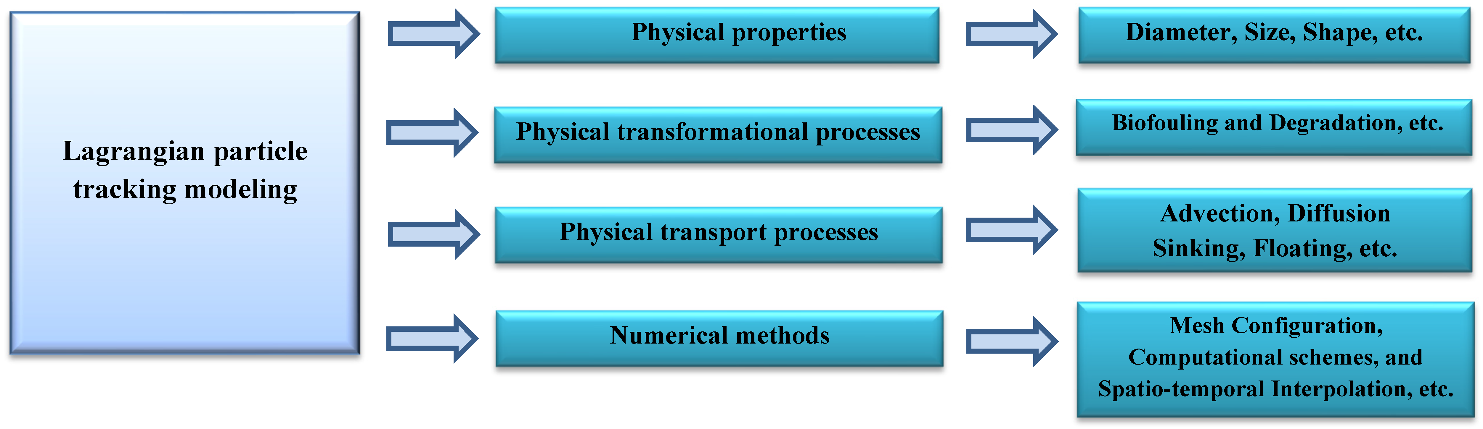
3. Physical Properties and Processes

3.1. Physical Properties

The behavior and transport of microplastics mainly depend on major physical properties including the size, density, and shape [44,66,96,99] of the particles. Microplastics are identified in varied sizes and shapes, and denser particles normally settle faster even with similar shapes and sizes [44]. Moreover, larger particles in terms of size but with the same density experience an increase in the ratio of the gravitational force applied on the particle to the fluid viscous resistance, which results in higher settling velocities and faster settling [61]. In addition, the shape of microplastics can affect their movements and settling velocity as well [100]. It has been observed that elongated particles such as films and fibers, known as larger particles, settle faster than smaller, circular particles [96]. Microplastics come in various regular (e.g., spherules, cylinders, and beads) and irregular shapes with different geometries (pellets and fibers). Regular shapes usually belong to primary microplastics while irregular shapes often can be seen among the secondary particles as a result of degradation [99]. Moreover, the physical properties of microplastics undergo changes due to the impacts of different processes and ambient factors such as algae invasion [101], salinity [102], UV index [103], temperature [103], and Stokes drift generated by wave action [104]. For instance, unlike freshly emitted particles, the edges of microplastics become smooth during aging as a result of mechanical degradation since they are under polishing imposed by other fragments [105]. Different equations used in the reviewed models for modeling hydrodynamic aspects (including microplastics’ physical properties) pertinent to the transport of microplastics have been summarized in this study in

Table 2. Various equations used for the modeling of hydrodynamic aspects in the reviewed models *.

No.	Mathematical or Empirical Relationships	Application	Defining Parameters	Employed in	Ref.
1	$v_s=c^n\times \left[A_0+A_{1}sin\left(\frac{2\pi \left(t+\varnothing \right)}{T}\right)\right]$	Settling velocity	$v_s$$({\mathrm{ms}}^{-1}$) is the settling velocity of each particle at time $t \left(\mathrm{hours}\right)$$,$ indicates the local concentration of particles $({\mathrm{kgm}}^{-3}$ $)$ is the exponent for adjusting concentration-dependent settling velocities, $A_0$ [106] is the non-cyclic component of the settling velocity $({\mathrm{ms}}^{-1}$)$, A_1$ represents the amplitude of a periodic sinusoidal variation in time $({\mathrm{ms}}^{-1}$)$,$ is the period of the sinusoidal variation $\left(\mathrm{hours}\right)$ and $\varnothing$ is the phase lag for the sinusoidal variation $(\mathrm{hours}$).	D-WAQ PART	[107]
2	$v_s=\frac{\vartheta }{2R}{d}_{*}^3{(38.1+0.93d_{*}^{12/7})}^{-7/8}$	Settling velocity of spherical particles	$\vartheta$ is the kinematic viscosity of water $({\mathrm{m}}^2{\mathrm{s}}^{-1}$$), d_{*}$ represents the dimensionless diameter of the particle, and $R$ is the radius of the particle $(\mathrm{mm})$.	TrackMPD	[99]
3	$d_{*}=2R{(g\left({\rho }_p-{\rho }_w\right)/{\rho }_w{\vartheta }^2)}^{1/3}$	Dimensionless diameter of the particle	$g$ is the gravitational acceleration $\left({\mathrm{ms}}^{-2}\right)$ and, ${\rho }_p$ and ${\rho }_w$ indicate the density of the particle and the suspending medium, respectively, with the same units $({\mathrm{gm}}^{-3})$.		[99]
4	$v_s=\frac{\pi }{2}\frac{1}{\vartheta }g\frac{\left({\rho }_p-{\rho }_w\right)}{{\rho }_w}\frac{2RL}{55.238L+12.691}$	Settling velocity of cylindrical particles	$L$ indicates the length of cylinders $(\mathrm{mm})$.		[99]
5	$v_s=\sqrt{\frac{4}{3}\frac{d}{C_D}\left|\frac{{\rho }_p-{\rho }_w}{{\rho }_w}\right|g}$	Settling velocity	$d$ is particle diameter $(\mathrm{mm})$$, {\rho }_p$$({\mathrm{gm}}^{-3})$ and ${\rho }_w$$({\mathrm{gm}}^{-3})$ indicate the density of the particle and the surrounding medium, respectively, $\mathrm{g}$ is the gravitational acceleration $\left({\mathrm{ms}}^{-2}\right)$ and, $C_D$ represents drag coefficient.	CaMPSim-3D	[98]
6	$\begin{array}{c}{C}_D\hfill \\ =\frac{24}{R{e}_p}{(\frac{1-\Psi }{R{e}_p}+1)}^{0.25}\hfill \\ +\frac{24}{R{e}_p}\left(0.1806R{e}_p{}^{0.6559}\right){\Psi }^{-R{e}_p{}^{0.08}}\hfill \\ +\frac{0.4251}{1+\frac{6880.95}{R{e}_p}{\Psi }^{5.05}}\hfill \end{array}$	Drag coefficient	$R{e}_p$ is particle Reynolds number and $\Psi$ is the particle shape factor [108]. Equation (6) has been reported as the best fit for modeling drag when interpreting microplastics’ sinking [109].		[98]

* The Ichthyop model uses the Stokes law in calculating the settling velocity.

.

3.2. Biofouling and Degradation (Physical Transformation Processes)

According to previous studies, microplastic particles are subjected to some natural transformation processes including fouling, degradation, and mechanical breakdown during their residence time in an aquatic ecosystem that may lead to changes in their physical properties [58]. Biofouling is controlled by different ambient environmental factors such as temperature, salinity, and the availability of sunlight, which is necessary for biofilm (including fine and ultrafine organisms and plankton) growth [76]. On the other hand, particles become more brittle and break apart into smaller pieces as a result of mechanical degradations by weathering, wave actions, interaction with other particles, the seabed, and the shore [110]. Degradation is typically a slow process that takes over 50 years to be fully completed for plastics since they are highly resistant to weathering [7,110]. However, in the swash zone [111] and some energetic coastal areas (e.g., salt marshes), natural abrasives including sediment and rock are present, and the degradation may be completed sooner, even within 8 weeks based on [112], thereby affecting seasonal microplastics’ transport. The main equations employed in the reviewed models in this study for considering biofouling and degradation processes are provided in

Table 3. The main equations used in the reviewed models for the consideration of biofouling and degradation.

No.	Mathematical or Empirical Relationships	Application	Defining Parameters	Employed in	Ref.
7	${\rho }_p={\rho }_0\frac{R_0^3}{{(R_0+BT)}^3}+{\rho }_D\left[1-\frac{R_0^3}{{(R_0+BT)}^3}\right]$	Biofouling of spherical particles	${\rho }_p$$({\mathrm{gm}}^{-3})$ is the density of a fouled spherical particle, ${\rho }_0$$({\mathrm{gm}}^{-3})$ is the density of a plastic particle, $R$$(\mathrm{mm})$ indicates microplastic radius, and $BT$ and ${\rho }_D$ represent the thickness $(\mathsf{\mu }\mathrm{m})$ and density $({\mathrm{gm}}^{-3})$ of a biofilm layer, respectively.	TrackMPD–CaMPSim-3D	[96]
8	${\rho }_p={\rho }_0\frac{R_0^2}{{(R_0+BT)}^2}+{\rho }_D\left[1-\frac{R_0^2}{{(R_0+BT)}^2}\right]$	Biofouling of cylindrical particles	${\rho }_p$$({\mathrm{gm}}^{-3})$ is the density of a fouled cylindrical particle, ${\rho }_0$$({\mathrm{gm}}^{-3})$ is the density of a plastic particle, $R$$(\mathrm{mm})$ indicates microplastic radius, and $BT$$\left(\mathsf{\mu }\mathrm{m}\right)$ and ${\rho }_D$$({\mathrm{gm}}^{-3})$ represent the thickness and density of a biofilm layer, respectively.	TrackMPD–CaMPSim-3D	[96]
9	$BT=B{T}_0+BR\mathrm{\Delta }t$	Biofouling	$B{T}_0$$\left(\mathsf{\mu }\mathrm{m}\right)$ is the thickness of initial biofouling, $BR$ is a constant biofilm thickness in stationary biofouling, and $\mathrm{\Delta }t$ indicates the time interval.	TrackMPD–CaMPSim-3D	[61]
10	$Size\left(D or L\right)=Siz{e}_0\left(1-DR·T/100\right)$	Degradation	$D$$(\mathrm{mm})$ and $L$$(\mathrm{mm})$ are the particle’s diameter and length, respectively. $Siz{e}_0$ indicates the particle’s initial diameter and length. $DR$ as a constant rate shows the percentage of decrease in size of the particle per day [112] and $T$ represents the duration of degradation from the beginning to the present time step.	TrackMPD–CaMPSim-3D	[61]

. It should be noted that none of the reviewed models are capable of simulating different types of aggregation.

3.3. Physical Transport Processes

In addition to the transformation processes (biofouling, degradation, aggregation), numerical fate and transport models can simulate different physical processes driving microplastics’ transport in water such as advection, diffusion, windage, resuspension, beaching, and washing-off. The transport of microplastics is generally governed by a generic advection–diffusion reaction, as follows [98]:

$$\frac{\partial C}{\partial t}=\nabla .\left(CU\right)+\nabla .\left(K\nabla CU\right)+\rho \left(C\right)$$

(11)

where $C$ indicates the concentration at time $t$, $U$ is the velocity of a surrounding medium, $K$ represents the dispersion coefficient, and $\rho \left(C\right)$ shows the reaction function.

Given the aforesaid concept, the main equations used in the reviewed models for addressing the main physical processes controlling microplastics’ transport in aquatic systems are provided in

Table 4. The mathematical or empirical equations employed in the reviewed models for considering the physical transport processes that microplastics undergo in aquatic environments.

No.	Mathematical or Empirical Relationships	Application	Defining Parameters	Employed in	Ref.
12	$\frac{d\stackrel{\rightharpoonup }{X}\left(t\right)}{dt}=\stackrel{\rightharpoonup }{u}\left(X, t\right)+\frac{d{\stackrel{\rightharpoonup }{X}}^{\prime }\left(t\right)}{dt}$	Trajectory Calculation	$\stackrel{\rightharpoonup }{X}$ is the 3D position vector with components in the horizontal plane, $d$ is the total derivative,$\stackrel{\rightharpoonup }{u}$ is the 3D velocity vector, and ${\stackrel{\rightharpoonup }{X}}^{\prime }$ is the fluctuation of the position vector.	D-WAQ PART	[58]
13	$V_{adv}=V_{flow}+V_{windage}$	Advection velocity	$V_{adv}$$\left({\mathrm{ms}}^{-1}\right)$ represents the velocity field, which is responsible for advection. $V_{flow}$$\left({\mathrm{ms}}^{-1}\right)$ is the velocity of flow, and $V_{windage}=C_{wd}\left(V_w-V_{flow}\right)$. ${\mathrm{C}}_{\mathrm{wd}}$ is an empirical wind drag coefficient that is related to particle characteristics and $V_w$$\left({\mathrm{ms}}^{-1}\right)$ represents the wind velocity at $10$ above sea level.		[58]
14	$K_{h\left(x,y\right)}=a{t}^b$	Turbulent horizontal component of the diffusion coefficient	$K_{h\left(x,y\right)}$ is the horizontal component of the diffusion coefficient $\left({\mathrm{m}}^2{\mathrm{s}}^{-1}\right)$ at time $t$ (which is defined from $t=0$ ), $a$ (which is equal to the dispersion coefficient for small $t$ ), and $b$$(\in \left[0, 1\right])$ are calibrating coefficients. It should be noted that the upper and lower limits of $K_{h\left(x,y\right)}$ are equal to $at$ and $a$ respectively, and $K_{h\left(x,y\right)}$ increases with time. It has been used in Equation (11).	D-WAQ PART	[113]
15	$D_z=\frac{c_{\mu }^{1/4}L\sqrt{k}}{{\sigma }_C}$	Turbulent vertical diffusion coefficient	$D_z$ is the vertical dispersion coefficient, ${\mathrm{C}}_{\mathsf{\mu }}$ indicates a calibrating constant for local equilibrium shear layers that is equal to 0.09, approximately. $L$ is the mixing length $\left(\mathrm{m}\right)$$,$ represents turbulent kinetic energy, and ${\sigma }_C$ is the Prandtl–Schmidt number. It has been used in Equation (11).	D-WAQ PART	[107]
16	$P={0.5}^{-t/T}$	The probability of being washed-off	$P$ is the probability of a particle being washed off, $t$ is the time step, and $T$ is the half-life of plastic litter.	D-WAQ PART—TrackMPD	[87]
17	$v_{part}=v_{water}+\frac{1}{24}g{d}^2\frac{\mathrm{\Delta }\rho }{{\rho }_w}{\vartheta }^{-1}\ln \left(\frac{2I}{d}+\frac{1}{2}\right)$	Vertical velocity of particle	$v_{water}$ is vertical velocity of water, $g$ is the gravitational force $\left({\mathrm{ms}}^{-2}\right)$, $d$ and $I$ are prolate spheroid axes (indicating the area of a particle), $\mathrm{\Delta }\rho ={\rho }_{part}-{\rho }_w$$, {\rho }_{part}$$({\mathrm{gm}}^{-3})$ is particle density and ${\rho }_w$$({\mathrm{gm}}^{-3})$ is the density of water, and $\vartheta$ indicates the kinematic viscosity.	Ichthyop	[114]
18	$K_h={\epsilon }^{1/3}{l}^{4/3}$	Horizontal turbulent diffusion coefficient	$\epsilon$ is the turbulent dissipation rate and $l$ is the cell size. It has been used in Equation (11).	Ichthyop	[115]
19	$x_{n+1}=x_n+U\mathrm{\Delta }{t}_i$ $y_{n+1}=y_n+V\mathrm{\Delta }{t}_i$ $z_{n+1}=z_n+W\mathrm{\Delta }{t}_i$	First-order Euler method for advection	$\mathrm{\Delta }{t}_i$ is an internal time interval and $U=\left(U,V,W\right)$ is the velocity vector. This is a first-order discretization of Equation (11).	TrackMPD	[61]
20	$x_{n+1}=x_n+R{(2r^{-1}{K}_h\mathrm{\Delta }{t}_i)}^{1/2}$	Calculation of horizontal displacement due to diffusion Equation (11)	$R$ indicates a random number with an average of zero and $r$ is its standard deviation that equals 1, and $K_h$ is horizontal diffusivity $({\mathrm{m}}^2{\mathrm{s}}^{-1}$).		[61]
21	$z_{n+1}=z_n+R{(2r^{-1}{K}_v\mathrm{\Delta }{t}_i)}^{1/2}$	Calculation of vertical diffusion term Equation (11)	$K_v$ is vertical diffusivity $({\mathrm{m}}^2{\mathrm{s}}^{-1}$).		[61]
22	$U=\frac{U_f+U_w\sqrt{\frac{{\rho }_{air}}{{\rho }_w} \frac{S_{above}}{S_{below}}}}{1+\sqrt{\frac{{\rho }_{air}}{{\rho }_w} \frac{S_{above}}{S_{below}}}}$	Velocity field as a function of current and wave velocities	$U_f$ is the current velocity, $U_w$ is the wind velocity, ${\rho }_{air}$ and ${\rho }_w$ indicate the density of air and water, $S_{above}$ and $S_{below}$ represent the cross-sectional areas of spherical and cylindrical particles in dry and wet conditions, respectively. Note that Equation (17) and (21) use the same principles and their difference is only in some coefficients.	TrackMPD	[61]
23	$\frac{S_{above}}{S_{below}}=\frac{2\pi }{\left(\alpha -sin\alpha \right)}-1$	The ratio of the dry cross-sectional area of the particles to its wet cross-sectional area.	$\alpha$ is defined by Equation (24).		[61]
24	$\alpha =2arcccos\left(1-\frac{h}{R}\right)$	Parameter for Equation (23)	$h$ is the Archimedean force, $R$ is the radius of the particle.		[61]
25	${\left(\frac{h}{R}\right)}^2·\left(3-\frac{h}{R}\right)=4\frac{\rho }{{\rho }_w}$	Archimedean force	$\rho$$({\mathrm{gm}}^{-3})$ and ${\rho }_w$$({\mathrm{gm}}^{-3})$ are the density of the particle and water, respectively.		[61]
26	$R_j=R_{jmax}\left(\frac{\tau }{{\tau }_{crit}}-1\right)$	Resuspension flux	$R_{jmax}$ is the maximum resuspension constant for microplastics. $\tau$ and ${\tau }_{crit}$ are shear stress and critical shear stress, respectively.	CaMPSim-3D	[116]
27	$\tau ={\rho }_w{(\frac{g^{0.5}{v}_w}{Chezy})}^2$	Actual shear stress	${\rho }_w$$({\mathrm{gm}}^{-3})$ is the density of seawater, $g$$\left({\mathrm{ms}}^{-2}\right)$ is gravitational acceleration, $v_w$ is the mean velocity of the seawater, and $Chezy$ is the Chezy coefficient $({\mathrm{m}}^{0.5}{\mathrm{s}}^{-1}$).		[116]
28	$v_p=\frac{{{\displaystyle \sum }}_{i=1}^6\frac{1}{{\propto }_i}{v}_i}{{{\displaystyle \sum }}_{i=1}^6\frac{1}{{\propto }_i}}+v_s$	Vertical displacement velocity of particles	where $v_p$ is the vertical displacement velocity of particles, $v_i$ is particle velocity at the computational cells, ${\propto }_i$ is vertex, and $v_s$ is particles settling/rising velocity (obtained from Equation (5)).	CaMPSim-3D	[98]
29	$Diff=\frac{\partial K}{\partial X}\mathrm{\Delta }t+R\left\{\sqrt{2K_p\left[X_p\left(t\right)+\frac{1}{2} \frac{\partial K}{\partial X}\mathrm{\Delta }t\right]\mathrm{\Delta }t}\right\}$	Calculation of diffusion term	where $K$ is the diffusion coefficient (obtained from Equation (14)), $\mathrm{\Delta }t$ is the time step, $R$ is a random number, and $K_p$ is the diffusion coefficient.		[98]

.

4. Numerical Lagrangian Models

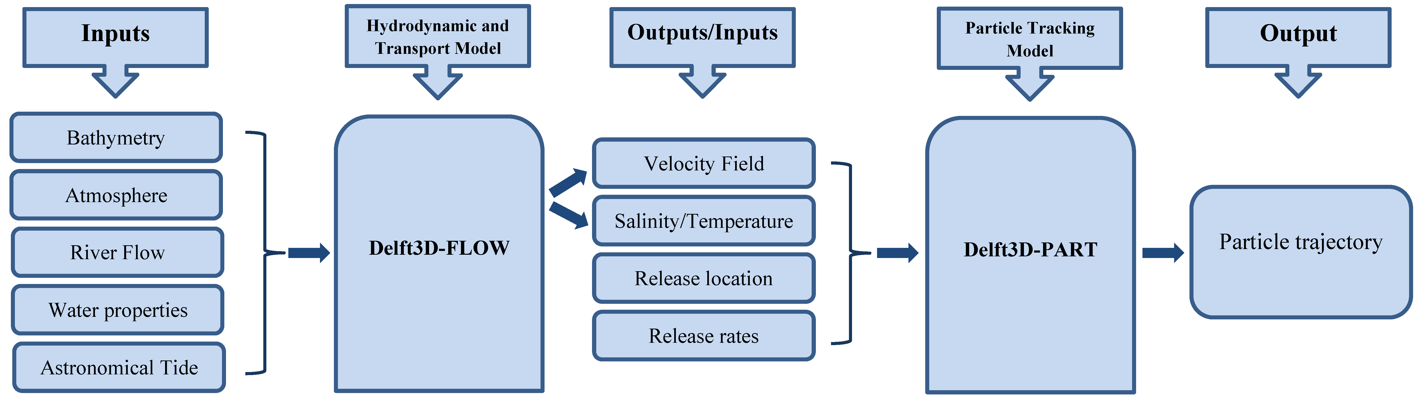
In PTM models, a velocity value is allocated to each particle. This is typically done by the interpolation of values from an Eulerian hydrodynamic model onto the position of microplastic particles. The advection velocity typically includes the settling velocity, the velocity of flow provided by the hydrodynamic model, and a diffusion-based velocity that is randomly generated, typically based on a Gaussian distribution [76,115]. Many PTM models use numerical methods such as the fourth-order Runge–Kutta method to solve equations in time.

In most PTM models, the number of required particles will be determined based on several factors such as the simulation period, the extent of particle dispersion, the cells’ size in the computational domain, computational resources, etc. [107].

The majority of PTM models calculate the settling velocity considering the impacts of the aforementioned physical properties such as density, size, and shape. The settling velocity of each particle, $v_s$, is defined based on the relationships, as shown in Table 2.

4.1. D-WAQ PART

Delft3D, as open-source software, can be applied for simulating flows, the transport of sediments, tidal currents, water quality, waves, etc. in various water settings. Delft3D has several modules as shown in Figure 2. The modules are linked to each other in order to simulate the multi-dimensional transport and hydrodynamics (in 2D or 3D) [117]. Particle transport and dynamical spatial distribution are simulated by the PART module of Delft3D using particle-tracking modeling using the inputs provided by the FLOW module (i.e., two- or three-dimensional flow data). In other words, velocity and other hydrodynamic parameters are computed by the FLOW module using an offline coupling and provided as inputs for the D-WAQ PART module.

D-WAQ PART is not capable of considering the impact of the biofouling process on the trajectories of micro-size particles via increasing the density and size of the particles since it cannot consider the thickness of the biofilm layer, and so, the density of a fouled particle. D-WAQ PART also lacks a specific tool to provide insight and appropriately predict complex processes including degradation as a long-term and aggregation as a short-term process.

Particle trajectories are computed over time in three dimensions by modeling the advection and dispersion processes [118]. As stated above, each individual particle can be advected by water currents and wind or wave drag as additional sources and also displaced randomly due to diffusion in order to explain unresolved processes.

The velocity of particles due to advection includes the local current velocity prepared by the hydrodynamic model in the Eulerian velocity field and the wind velocity at the location of a particle as shown in Equation (13) [58]. The wind-drag coefficient is related to object characteristics as an empirical parameter. In addition, D-WAQ PART employs a random-walk particle-tracking model in order to describe the movement of particles due to diffusion processes. The diffusion is described using kinetic gas theory and the theory of Brownian motion [107].

D-WAQ PART addresses beaching and washing-off using the probability of being washed off, as shown in Equation (16).

Many numerical models, including D-WAQ PART, are not capable of reading the unstructured mesh information provided by an Eulerian model. However, some of the other Delft-3D modules (e.g., D-Water Quality and GPP) can solve the advection–diffusion equation numerically on arbitrary, unstructured grids and structured, shaped grids such as triangles, rectangles, and curved elements.

On the other hand, D-WAQ PART utilizes the linear and block interpolation implemented for all time functions between time intervals [107]. In the linear interpolation, D-WAQ PART interpolates the hydrodynamic inputs linearly between the time records while it interpolates the two different subsequent inputs with similar time as the block interpolation.

4.2. Ichthyop

Ichthyop is a free Java-based particle tracking numerical model which was originally developed to study ichthyoplankton dynamics [97]. Ichthyop has also been employed for modeling the fate and transport of microplastics and toxic algae [76,119]. The model can use three-dimensional hydrodynamic information including temperature, velocity, and salinity, simulated by oceanic numerical models such as the Regional Oceanic Modelling System, called ROMS, and the Model for Applications at Regional Scale, named MARS, as input [97]. Ichthyop is capable of providing two types of microplastics simulations: (1) modeling plastic particle trajectories, and (2) ensemble simulation (i.e., executing a series of numerous particle tracking simulations) [97]. Ichthyop can also simulate the trajectory of more than one million particles as passive tracers [119].

Similar to D-WAQ PART, Ichthyop does not consider the integration of complex particle transformation processes including biofouling, different types of aggregation, degradation, and fragmentation.

Ichthyop uses the Runge–Kutta method [97] for solving the advection equation [76]. Horizontal and vertical advection and dispersion can be simulated in Ichthyop [76,97,113,119,120]. The model follows D-WAQ PART and uses Equation (11) to simulate the horizontal advection. Ichthyop utilizes a terminal velocity ($v_{part}$) in order to address the vertical movement of particles, as defined in Equation (17) [114].

Ichthyop uses Equation (18) for the consideration of horizontal diffusion. Accordingly, horizontal diffusion is defined as a function of the turbulent dissipation rate and the cell size of the computational domain [115]. Furthermore, the vertical diffusion of particles is predicted based on a proposed random-walk simulation [121].

Ichthyop is incapable of simulating some other effective physical processes on microplastics’ fate and transport, such as beaching and washing-off, windage, resuspension, and aggregation, which can be regarded as an important limitation.

Hydrodynamic parameters are simulated on a rectangular structured mesh in some hydrodynamic models such as ROMS and MARS. Then, they are interpolated linearly and extracted at time steps in order to be prepared as inputs for Ichthyop.

4.3. TrackMPD

Amongst the three-dimensional numerical models, TrackMPD is an open-source model that has been released in recent years [61] based on the framework of the Particle Tracking and Analysis Toolbox (PaTATO) [122]. TrackMPD is compatible with various ocean models in order to address the fate and transport of marine microplastic debris in coastal areas. TrackMPD is capable of simulating microplastics’ behavior in three dimensions considering different physical processes, including beaching and washing-off, biofouling and degradation, advection, windage, turbulent dispersion, and sinking, as well as different physical properties such as density (Equations (7) and (8)), size (Equation (10)), and shape (Equations (2)–(4), (7) and (8)). The physical properties of microplastics can be parametrized in TrackMPD, particularly in the calculation of the settling velocity. TrackMPD utilizes the empirical equations of [99] and [123] in estimating the settling velocity of microplastics with different shapes as a function of particle density and radius. Accordingly, the settling velocity ($v_s$) of spherical particles (${\mathrm{ms}}^{-1}$) is obtained based on a calibrated formulation provided by [123], as shown in Equations (2) and (3), while this is different, as determined in Equation (4), for cylindrical fragments (${\mathrm{mms}}^{-1}$) [99].

The effects of biofouling on the fate and transport of microplastics can be investigated by TrackMPD. In other words, TrackMPD uses some empirical equations in order to approximate the thickness of the biofilm layer. In this respect, the thickness of biofilm layers of spherical and cylindrical particles can be estimated based on Equations (7) and (8), respectively [96]. Accordingly, biofilm thickness can be given either a constant or variable value over time. The case of constant biofilm thickness is referred to as stationary biofouling, while the case of variable biofilm thickness is considered as non-stationary biofouling.

TrackMPD simply predicts mechanical degradation by using an empirical relation (Equation (10)). In this respect, the size of plastic particles (their diameter or length) decreases based on a constant rate and time. While TrackMPD can simulate biofouling and degradation, it suffers from incapability in simulating some other transformational processes such as hetero- and homo-aggregation.

To simulate the horizontal and vertical movements of plastic particles due to advection, TrackMPD employs the Runge–Kutta method [61]. In this respect, the velocity of the flow is calculated iteratively in three directions at the location of a particle to consider velocity values (${\mathrm{ms}}^{-1}$) at past and future times. Then, to calculate particle displacements ($\mathrm{m}$) and obtain their new location in each direction, the previous location of microplastics is added to the multiplication of the internal time interval ($\mathrm{\Delta }{t}_i$) and the flow velocity’s components ($U=\left(u,v,w\right)$), as shown in Equation (19). Moreover, the horizontal (in $x$ or $y$ directions) and vertical diffusion of particles is predicted in TrackMPD based on a random-walk model, as demonstrated in Equation (20) and (21), respectively [61].

As with D-WAQ PART, TrackMPD can consider the windage effect in the calculation of particle velocity. Accordingly, the horizontal wind-induced drift of microplastics is considered using Equations (22)–(25) [61].

TrackMPD estimates the probability of microplastics’ washing-off based on a Monte Carlo method, as shown in Equation (16) [61]. The probability ($P$) of being washed off in TrackMPD is an exponential function of the time step ($t$), and the half-life of plastic litter ($T$) is equal to the time that microplastics remain on the beach [87]. If $P$ is higher than a random number, which varies from 0 to 1, beached microplastics can be transported (i.e., washed off) seaward at extreme tides. D-WAQ PART uses a basically similar approach in the calculation of the probability of wash-off.

Currently, TrackMPD can read hydrodynamic parameters off-line from some models such as ROMS in only a rectangular structured mesh. Moreover, hydrological properties are interpolated spatially at each time step, and then the hydrodynamic model assigns the values to particles located in the corresponding grid cells of TrackMPD [61].

4.4. CaMPSim-3D

Canadian microplastic simulation (CaMPSim), the newest three-dimensional Eulerian–Lagrangian framework [98], has been developed recently for simulating microplastics’ fate and transport in different aquatic environments. CaMPSim-3D is based on the coupling of a three-dimensional Lagrangian particle-tracking model and TELEMAC modeling system as the Eulerian hydrodynamic numerical model. Similar to procedures followed by the aforesaid models, hydrodynamic inputs such as atmospheric pressure, the direction and speed of the wind, hydrodynamic and water quality parameters (including velocity, temperature, salinity, water level, and algae concentration), wave height and direction as well as its time period, and characteristics of suspended sediments that are all prepared by the Eulerian model are fed into the Lagrangian particle-tracking model. On the other hand, CaMPSim-3D considers the physical properties of microplastics (such as density, size, and shape) and physical processes (including the effect of positive/negative buoyancy, advection, biofouling, spatio-temporal varying diffusion, degradation, washing-off, and beaching, etc.).

In CaMPSim-3D, the physical properties of plastic particles such as density, diameter, gravity, and shape are parameterized in the calculation of the rising or settling velocity. Unlike TrackMPD, the formulation employed in CaMPSim-3D for calculating the settling velocity can be used for particles with different shapes, such as spherules, films, fragments, and fibers [98]. CaMPSim-3D calculates the settling velocity ($v_s$) based on force balance formulation Equations (5) and (6) provided for Newtonian fluids [98]. CaMPSim-3D can predict the formation of biofilm layers on plastic particles. In this respect, CaMPSim-3D utilizes some proposed empirical equations for estimating the biofilm thickness, e.g., Equations (7)–(9). In addition, CaMPSim-3D considers the degradation of microplastics based on empirical relationships provided in the literature, e.g., Equation (10). However, it cannot simulate both types of aggregation (i.e., hetero- and homo-aggregation) that microplastics undergo.

As with some of the aforementioned models, the Lagrangian particle-tracking model, CaMPSim-3D, can simulate not only the advection and diffusion of particles but also beaching and washing-off. It is also capable of considering the effect of buoyancy on particle movement [98]. In CaMPSim-3D, the displacement of particles due to horizontal and vertical advection is calculated by solving the first- to the fourth-order of Equations (19)–(21). In addition, the vertical displacement velocity of particles ($v_p$) is calculated based on the vertical component of flow velocity, and particle settling/rising velocity ($v_s$, obtained from Equation (5)), as shown in Equation (28) [98]. Furthermore, CaMPSim-3D considers the impact of wind as a driving factor on the transport of microplastics (see Equations (20)–(22). The turbulent diffusion of plastic particles is simulated in CaMPSim-3D by using a modified relationship, as shown in Equation (29) as a function of $K$ (diffusion coefficient, see Equation (14)), $\mathrm{\Delta }t$ (the time step), $R$ (a random number obtained from a normal distribution, which varies between −1 and 1), and $K_p$ (diffusion coefficient at $X_p$ as a function of $t$) [98].

$K_p$ is calculated using the eddy viscosity (${\vartheta }_t$) calculated by the Eulerian hydrodynamic model [98]. Moreover, CaMPSim-3D predicts resuspension and deposition as well as beaching and washing-off using the proposed relationships (see Equation (16)).

One of the advantages of CaMPSim-3D, in comparison with the aforesaid models, is its ability to employ an unstructured grid [98]. It should be mentioned that the CaMPSim-3D model reads hydrodynamic parameters from an Eulerian hydrodynamic model (TELEMAC). Although this approach has some benefits by reducing interpolation errors, it imposes more computational time for point locations in an unstructured mesh. Furthermore, CaMPSim-3D employs an inverse distance-weighted method for the interpolation (or map) of hydrodynamic inputs in space, which is implemented for each particle [98].

5. Results and Discussion

Despite the fact that the reviewed models have generally acceptable accuracy in simulating the physical transformational and transport processes, each has some noticeable limitations in this regard. In this section, we have tried to discuss the reviewed models’ limitations in detail regarding the consideration of microplastics’ physical properties and processes. It can be concluded that this section can give better insights into the current gaps in the reviewed models.

D-WAQ PART and Ichthyop assume microplastics as passive particles without inertia when they are floated at the sea surface, which is different in real ocean conditions [58,119] since the shape and geometry of microplastics have impacts on their behavior, particularly during the different physical processes that they undergo. TrackMPD considers plastic particles as both active and passive particles using different scenarios. It means TrackMPD can simulate microplastics with different shapes (spherical and cylindrical) and sizes [61]. CaMPSim-3D is more powerful in this regard in comparison with the aforesaid models. This is because it utilizes the shape factor ($\Psi$) which capable CaMPSim-3D in considering particles with different sphericity and circularity [98].

As stated in Section 4, D-WAQ PART and Ichthyop cannot simulate biofouling and degradation, while both TrackMPD and CaMPSim-3D are capable of simulating these processes using the same empirical relationships. It should be noted that TrackMPD and CaMPSim-3D cannot simulate biofouling and degradation together within the same simulation. On the other hand, there are some other transformational processes in the real ocean condition such as hetero- and homo-aggregation [124] and agglomeration (known as the formation of particle clusters in which weak physical interactions are dominant between particles [125]). In addition, microplastics undergo weathering, photodegradation, chemical and biological degradation, and defouling (known as the biofilm layer disintegration [44]) in real conditions. However, none of the reviewed models can simulate any of the aforementioned processes yet.

Unlike Ichthyop, D-WAQ PART, TrackMPD, and CaMPSim-3D can predict beaching and washing-off using a probability empirical theory with the same accuracy. However, actual beaching and washing-off in the real condition are highly complex processes since they depend on many other factors, such as the characteristics of winds, tides, waves, and coastline structure [58]. Moreover, microplastics may undergo stranding at the shoreline and be washed off from it repeatedly in subsequent episodes. Accordingly, the aforesaid models are currently incapable of simulating beaching and washing-off more accurately.

All of the reviewed models can predict advection and diffusion; however, their accuracy in this regard is different. All models can simulate advection and windage (except for Ichthyop). Moreover, all of them are capable of modeling horizontal and vertical diffusion, although some of them employ different methods and relationships in calculating the horizontal/vertical diffusion coefficient. However, CaMPSim-3D utilizes a modified relationship for the calculation of turbulent diffusion, which seems to be a more accurate approach in comparison with the methods employed by other models. Among the reviewed models, only CaMPSim-3D can predict resuspension. On the other hand, there are some additional important driving transport processes such as Stokes drift (as a result of wave action [58,104]), burial into the deep sediment of the waterbodies [124], and remobilization [126], which none of the reviewed models can predict.

All of the reviewed models (except for CaMPSim-3D) are incapable of reading hydrodynamic parameters from an unstructured mesh provided by an Eulerian model. It should be noted that although reading hydrodynamic data from an unstructured mesh leads to a decrease in interpolation errors, it increases the computational costs of particle-tracking simulations.

D-WAQ PART and TrackMPD can read and then simulate spatio-temporally interpolated hydrodynamic parameters, while Ichthyop is only capable of utilizing temporally interpolated data. CaMPSim-3D can consider only spatially interpolated hydrodynamic values in the particle-tracking of plastic particles. It seems D-WAQ PART and TrackMPD utilize more accurate numerical schemes in this regard. On the other hand, the efficiency and computational speed of each of the reviewed models can be compared in systematic case studies. It should be noted that there are other numerical models such as TRACMASS and OceanParcels which have not been reviewed in this paper for the sake of briefness and to focus on models with more capabilities.

To make a general comparison among the reviewed models, the main characteristics and capabilities of the reviewed models have been summarized in

Table 5. Summary of the main information of the reviewed models.

Particle-Tracking Model	Open Access (Free to Use)	Application (Particle Tracking of)	Shape and Type of the Simulated Particles	Main Mechanism Can Be Simulated	Initial Year of Release *	Ref.
D-WAQ PART	No	Microplastics, Sediments (first-order decaying substances)	Different shapes and types	Advection (and windage), Diffusion, Beaching and washing-off, Sinking	2019	[75,77]
Ichthyop	Yes	Microplastics	Prolate spheroids	Advection, Diffusion, Sinking	2008	[76,97]
TrackMPD	Yes	Microplastics	Spherical and cylindrical particles	Advection (and windage), Diffusion, Beaching and washing-off, Sinking, Biofouling, Degradation	2019	[61]
CaMPSim-3D	Yes	Microplastics	Spherules, films, fragments, and fibers	Advection (and windage), Diffusion, Beaching and washing-off, Sinking, Biofouling, Degradation	2021	[98]

* Based on the publication date of the paper which introduces the model.

. It can be seen which of the reviewed models are free for non-commercial use. Moreover, the capability of the reviewed models in terms of the particle tracking of what type and shape of particles have been compared. In addition, the main physical transformational and transport process each model can simulate are shown.

6. Conclusions and Future Research Directions

The current study aims, as a worthwhile endeavor, to systematically review some well-known Lagrangian numerical particle-tracking models that have been used for predicting the fate and transport of microplastics. In this regard, four Lagrangian particle-tracking models, i.e., D-WAQ PART, Ichthyop, TrackMPD, and CaMPSim-3D, have been investigated in terms of addressing physical transport processes (advection, diffusion, windage, beaching and washing-off, and resuspension) and physical transformation processes (biofouling and degradation) with consideration of the effects of the physical properties (mainly size, diameter, and shape) of microplastics on their fate and transport. Moreover, a numerical scheme of each model is described based on its spatio-temporal interpolation scheme and the structure of the adopted mesh. Accordingly, it has been shown that some of these models are more powerful than others in capturing the physical properties of particles and predicting their behavior under different physical transport and transformation processes. Some concluding remarks for the current study are summarized below:

• With respect to the consideration of the physical properties of microplastics, D-WAQ PART and Ichthyop use simplified equations for calculating the settling velocity as a function of the size and density of plastic particles, while TrackMPD and CaMPSim-3D employ more accurate equations to meet the effect of particle shape as well. In other words, D-WAQ PART utilizes an equation for calculating the settling velocity of plastic particles with different shapes and types, while Ichthyop is suited for considering the settling velocity of prolate spheroids. TrackMPD can differentiate spherical and cylindrical particles in the simulation of the settling velocity. CaMPSim-3D can be applied for simulating particles with different shapes, including spherules, films, fragments, and fibers.
• Among the transformation processes reviewed in this study (i.e., biofouling and degradation), although biofouling has been regarded as one of the important processes in the fate of microplastics, D-WAQ PART and Ichthyop are unable to predict the behavior of particles under the influence of this process. However, TrackMPD and CaMPSim-3D can simulate fouled particles using empirical equations. Unlike D-WAQ PART and Ichthyop, TrackMPD, and CaMPSim-3D can predict the degradation of microplastics based on the proposed relationship in the literature.
• Four particle-tracking models employ generally universal advection–diffusion equations, while the equations for parameterizing various physical processes may be different. However, only D-WAQ PART, TrackMPD, and CaMPSim-3D consider the effect of wind-induced drift as an additional term of advection. In addition, all models are capable of meeting horizontal and vertical diffusion (dispersion). All reviewed models use spatio-temporally varying diffusion coefficients. D-WAQ PART, TrackMPD, and CaMPSim-3D can predict beaching and washing-off using some probability-based relationships.
• D-WAQ PART, Ichthyop, and TrackMPD can read the extracted hydrodynamic data and simulate particle behavior and particle trajectories only on a structured mesh, while CaMPSim-3D reads hydrodynamic data from an unstructured mesh system. Moreover, the hydrodynamic data are only interpolated linearly at each time step and prepared as inputs for Ichthyop. D-WAQ PART and TrackMPD utilize the spatio-temporal interpolation of the current characteristics, while CaMPSim-3D can use only spatially interpolated data.

Given the aforesaid descriptions, there are some physical transport and transformation processes that some of the studied models are unable to simulate or exhibit less accuracy for in modeling. In fact, in order to understand the impacts of microplastics on the sustainability of water resources comprehensively, with higher levels of accuracy, we need to fully understand their behavior, which can be elucidated by using a versatile and accurate modeling system. None of the reviewed models can simulate homo- and hetero-aggregation or agglomeration. None of the four models can predict photodegradation or chemical and biological degradation as important processes in the fate of plastic particles. Wave-induced drift as an additional advection is observed only in CaMPSim-3D. It is suggested that further studies be conducted in order to expand the current knowledge of microplastics’ fate and transport. There are some important processes that need to be further studied with regard to the behavior of microplastics in the real condition (e.g., hetero- and homo-aggregation, agglomeration, weathering, photodegradation, chemical and biological degradation, defouling, resuspension, Stokes drift, and remobilization). More in-depth studies, as well as more accurate numerical models in capturing the microplastics’ behavior, along with significant modifications in the numerical simulation structure of the reviewed models, are recommended for the future.

References

1. Panno, S.V.; Kelly, W.R.; Scott, J.; Zheng, W.; McNeish, R.E.; Holm, N.; Hoellein, T.J.; Baranski, E.L. Microplastic contamination in karst groundwater systems. Groundwater 2019, 57, 189–196. [Google Scholar] [CrossRef] [PubMed]
2. Bergmann, M.; Gutow, L.; Klages, M. Marine Anthropogenic Litter; Springer: Berlin/Heidelberg, Germany, 2015. [Google Scholar]
3. Wagner, M.; Lambert, S. Freshwater Microplastics: Emerging Environmental Contaminants? Springer: Berlin/Heidelberg, Germany, 2018. [Google Scholar]
4. Hartmann, N.B.; Nolte, T.; Sørensen, M.A.; Jensen, P.R.; Baun, A. Aquatic ecotoxicity testing of nanoplastics. Lessons Learned From Nanoecotoxicology; DTU Environment, Technical University of Denmark: Kongens Lyngby, Denmark, 2015. [Google Scholar]
5. Rocha-Santos, T.; Duarte, A.C. A critical overview of the analytical approaches to the occurrence, the fate and the behavior of microplastics in the environment. Trends Anal. Chem. 2015, 65, 47–53. [Google Scholar] [CrossRef]
6. Euopean Commission. Environmental and Health Risks of Microplastic Pollution; European Commission: Brussels, Belgium, 2019. [Google Scholar]
7. Barnes, D.K.; Galgani, F.; Thompson, R.C.; Barlaz, M. Accumulation and fragmentation of plastic debris in global environments. Philos. Trans. R. Soc. B Biol. Sci. 2009, 364, 1985–1998. [Google Scholar] [CrossRef] [Green Version]
8. Koelmans, A.A.; Bakir, A.; Burton, G.A.; Janssen, C.R. Microplastic as a vector for chemicals in the aquatic environment: Critical review and model-supported reinterpretation of empirical studies. Environ. Sci. Technol. 2016, 50, 3315–3326. [Google Scholar] [CrossRef] [PubMed]
9. Ryan, P.G.; Moore, C.J.; Van Franeker, J.A.; Moloney, C.L. Monitoring the abundance of plastic debris in the marine environment. Philos. Trans. R. Soc. B Biol. Sci. 2009, 364, 1999–2012. [Google Scholar] [CrossRef] [PubMed] [Green Version]
10. Thevenon, F.; Carroll, C.; Sousa, J. Plastic Debris in the Ocean: The Characterization of Marine Plastics and Their Environmental Impacts, Situation Analysis Report; IUCN: Gland, Switzerland, 2014; Volume 52. [Google Scholar]
11. Wright, S.L.; Thompson, R.C.; Galloway, T.S. The physical impacts of microplastics on marine organisms: A review. Environ. Pollut. 2013, 178, 483–492. [Google Scholar] [CrossRef] [PubMed]
12. Wright, S.L.; Kelly, F.J. Plastic and human health: A micro issue? Environ. Sci. Technol. 2017, 51, 6634–6647. [Google Scholar] [CrossRef]
13. Lithner, D.; Larsson, Å.; Dave, G. Environmental and health hazard ranking and assessment of plastic polymers based on chemical composition. Sci. Total Environ. 2011, 409, 3309–3324. [Google Scholar] [CrossRef]
14. Rochman, C.M.; Browne, M.A.; Halpern, B.S.; Hentschel, B.T.; Hoh, E.; Karapanagioti, H.K.; Rios-Mendoza, L.M.; Takada, H.; Teh, S.; Thompson, R.C. Classify plastic waste as hazardous. Nature 2013, 494, 169–171. [Google Scholar] [CrossRef]
15. Napper, I.E.; Thompson, R.C. Marine plastic pollution: Other than microplastic. In Waste; Elsevier: Amsterdam, The Netherlands, 2019. [Google Scholar]
16. Nikpay, M. Wastewater Fines Influence the Adsorption Behavior of Pollutants onto Microplastics. J. Polym. Environ. 2022, 32, 776–783. [Google Scholar] [CrossRef]
17. Bakir, A.; Rowland, S.J.; Thompson, R.C. Transport of persistent organic pollutants by microplastics in estuarine conditions. Estuar. Coast. Shelf Sci. 2014, 140, 14–21. [Google Scholar] [CrossRef] [Green Version]
18. Cole, M.; Lindeque, P.; Halsband, C.; Galloway, T.S. Microplastics as contaminants in the marine environment: A review. Mar. Pollut. Bull. 2011, 62, 2588–2597. [Google Scholar] [CrossRef] [PubMed]
19. Gall, S.C.; Thompson, R.C. The impact of debris on marine life. Mar. Pollut. Bull. 2015, 92, 170–179. [Google Scholar] [CrossRef] [PubMed]
20. Galgani, F.; Hanke, G.; Werner, S.D.V.L.; De Vrees, L. Marine litter within the European marine strategy framework directive. ICES J. Mar. Sci. 2013, 70, 1055–1064. [Google Scholar] [CrossRef]
21. Thompson, R.C.; Moore, C.J.; Vom Saal, F.S.; Swan, S.H. Plastics, the environment and human health: Current consensus and future trends. Philos. Trans. R. Soc. B Biol. Sci. 2009, 364, 2153–2166. [Google Scholar] [CrossRef]
22. Eerkes-Medrano, D.; Thompson, R.C.; Aldridge, D.C. Microplastics in freshwater systems: A review of the emerging threats, identification of knowledge gaps and prioritisation of research needs. Water Res. 2015, 75, 63–82. [Google Scholar] [CrossRef]
23. Eriksen, M.; Mason, S.; Wilson, S.; Box, C.; Zellers, A.; Edwards, W.; Farley, H.; Amato, S. Microplastic pollution in the surface waters of the Laurentian Great Lakes. Mar. Pollut. Bull. 2013, 77, 177–182. [Google Scholar] [CrossRef]
24. Li, J.; Liu, H.; Chen, J.P. Microplastics in freshwater systems: A review on occurrence, environmental effects, and methods for microplastics detection. Water Res. 2018, 137, 362–374. [Google Scholar] [CrossRef]
25. Jeftic, L.; Sheavly, S.; Adler, E.; Meith, N. Marine Litter: A Global Challenge; UNEP: Nairobi, Kenya, 2009. [Google Scholar]
26. Galgani, F.; Hanke, G.; Maes, T. Global Distribution, Composition and Abundance of Marine Litter, in Marine Anthropogenic Litter; Springer: Cham, Switzerland, 2015; pp. 29–56. [Google Scholar]
27. Ivar do Sul, J.A.; Costa, M.F. Plastic pollution risks in an estuarine conservation unit. J. Coast. Res. 2013, 65, 48–53. [Google Scholar] [CrossRef]
28. Li, Y.; Zhang, H.; Tang, C. A review of possible pathways of marine microplastics transport in the ocean. Anthr. Coasts 2020, 3, 6–13. [Google Scholar] [CrossRef] [Green Version]
29. Desforges, J.P.W.; Galbraith, M.; Dangerfield, N.; Ross, P.S. Widespread distribution of microplastics in subsurface seawater in the NE Pacific Ocean. Mar. Pollut. Bull. 2014, 79, 94–99. [Google Scholar] [CrossRef] [PubMed]
30. Woodall, L.C.; Sanchez-Vidal, A.; Canals, M.; Paterson, G.L.; Coppock, R.; Sleight, V.; Calafat, A.; Rogers, A.D.; Narayanaswamy, B.E.; Thompson, R.C. The deep sea is a major sink for microplastic debris. R. Soc. Open Sci. 2014, 1, 140317. [Google Scholar] [CrossRef] [PubMed] [Green Version]
31. Free, C.M.; Jensen, O.P.; Mason, S.A.; Eriksen, M.; Williamson, N.J.; Boldgiv, B. High-levels of microplastic pollution in a large, remote, mountain lake. Mar. Pollut. Bull. 2014, 85, 156–163. [Google Scholar] [CrossRef] [PubMed]
32. McCormick, A.; Hoellein, T.J.; Mason, S.A.; Schluep, J.; Kelly, J.J. Microplastic is an abundant and distinct microbial habitat in an urban river. Environ. Sci. Technol. 2014, 48, 11863–11871. [Google Scholar] [CrossRef] [PubMed]
33. Klein, S.; Worch, E.; Knepper, T.P. Occurrence and spatial distribution of microplastics in river shore sediments of the Rhine-Main area in Germany. Environ. Sci. Technol. 2015, 49, 6070–6076. [Google Scholar] [CrossRef]
34. Lechner, A.; Keckeis, H.; Lumesberger-Loisl, F.; Zens, B.; Krusch, R.; Tritthart, M.; Glas, M.; Schludermann, E. The Danube so colourful: A potpourri of plastic litter outnumbers fish larvae in Europe’s second largest river. Environ. Pollut. 2014, 188, 177–181. [Google Scholar] [CrossRef] [Green Version]
35. Yonkos, L.T.; Friedel, E.A.; Perez-Reyes, A.C.; Ghosal, S.; Arthur, C.D. Microplastics in four estuarine rivers in the Chesapeake Bay, USA. Environ. Sci. Technol. 2014, 48, 14195–14202. [Google Scholar] [CrossRef]
36. Kooi, M.; Reisser, J.; Slat, B.; Ferrari, F.F.; Schmid, M.S.; Cunsolo, S.; Brambini, R.; Noble, K.; Sirks, L.A.; Linders, T.E.; et al. The effect of particle properties on the depth profile of buoyant plastics in the ocean. Sci. Rep. 2016, 6, 1–10. [Google Scholar] [CrossRef] [Green Version]
37. Browne, M.A.; Crump, P.; Niven, S.J.; Teuten, E.; Tonkin, A.; Galloway, T.; Thompson, R. Accumulation of microplastic on shorelines woldwide: Sources and sinks. Environ. Sci. Technol. 2011, 45, 9175–9179. [Google Scholar] [CrossRef]
38. Lorenzo-Navarro, J.; Castrillón-Santana, M.; Sánchez-Nielsen, E.; Zarco, B.; Herrera, A.; Martínez, I.; Gómez, M. Deep learning approach for automatic microplastics counting and classification. Sci. Total Environ. 2021, 765, 142728. [Google Scholar] [CrossRef]
39. Girshick, R.; Donahue, J.; Darrell, T.; Malik, J. Rich feature hierarchies for accurate object detection and semantic segmentation. In Proceedings of the IEEE Conference on Computer Vision and Pattern Recognition, Columbus, OH, USA, 23–28 June 2014. [Google Scholar]
40. Girshick, R. Fast r-cnn. In Proceedings of the IEEE International Conference on Computer Vision, Santiago, Chile, 7–13 December 2015. [Google Scholar]
41. Ren, S.; He, K.; Girshick, R.; Sun, J. Faster r-cnn: Towards real-time object detection with region proposal networks. Adv. Neural Inf. Process. Syst. 2015, 28, 91–99. [Google Scholar] [CrossRef] [PubMed] [Green Version]
42. Redmon, J.; Divvala, S.; Girshick, R.; Farhadi, A. You only look once: Unified, real-time object detection. In Proceedings of the IEEE Conference on Computer Vision and Pattern Recognition, Las Vegas, NV, USA, 27–30 June 2016. [Google Scholar]
43. Liu, W.; Anguelov, D.; Erhan, D.; Szegedy, C.; Reed, S.; Fu, C.Y.; Berg, A.C. Ssd: Single Shot Multibox Detector. In European Conference on Computer Vision; Springer: Berlin/Heidelberg, Germany, 2016. [Google Scholar]
44. Kooi, M.; Nes, E.H.V.; Scheffer, M.; Koelmans, A.A. Ups and downs in the ocean: Effects of biofouling on vertical transport of microplastics. Environ. Sci. Technol. 2017, 51, 7963–7971. [Google Scholar] [CrossRef] [PubMed] [Green Version]
45. Atugoda, T.; Piyumali, H.; Liyanage, S.; Mahatantila, K.; Vithanage, M. Fate and Behavior of Microplastics in Freshwater Systems. In Handbook of Microplastics in the Environment; Springer: Berlin/Heidelberg, Germany, 2020; pp. 1–31. [Google Scholar]
46. Besseling, E.; Quik, J.T.; Sun, M.; Koelmans, A.A. Fate of nano-and microplastic in freshwater systems: A modeling study. Environ. Pollut. 2017, 220, 540–548. [Google Scholar] [CrossRef]
47. Van Sebille, E.; Aliani, S.; Law, K.L.; Maximenko, N.; Alsina, J.M.; Bagaev, A.; Bergmann, M.; Chapron, B.; Chubarenko, I.; Cózar, A.; et al. The physical oceanography of the transport of floating marine debris. Environ. Res. Lett. 2020, 15, 23003. [Google Scholar] [CrossRef] [Green Version]
48. Rummel, C.D.; Jahnke, A.; Gorokhova, E.; Kühnel, D.; Schmitt-Jansen, M. Impacts of biofilm formation on the fate and potential effects of microplastic in the aquatic environment. Environ. Sci. Technol. Lett. 2017, 4, 258–267. [Google Scholar] [CrossRef] [Green Version]
49. Ryan, P.G. Does size and buoyancy affect the long-distance transport of floating debris? Environ. Res. Lett. 2015, 10, 84019. [Google Scholar] [CrossRef]
50. Eriksen, M.; Lebreton, L.C.; Carson, H.S.; Thiel, M.; Moore, C.J.; Borerro, J.C.; Galgani, F.; Ryan, P.G.; Reisser, J. Plastic pollution in the world’s oceans: More than 5 trillion plastic pieces weighing over 250,000 tons afloat at sea. PLoS ONE 2014, 9, e111913. [Google Scholar] [CrossRef] [PubMed] [Green Version]
51. Obbard, R.W.; Sadri, S.; Wong, Y.Q.; Khitun, A.A.; Baker, I.; Thompson, R.C. Global warming releases microplastic legacy frozen in Arctic Sea ice. Earth’s Future 2014, 2, 315–320. [Google Scholar] [CrossRef]
52. Waller, C.L.; Griffiths, H.J.; Waluda, C.M.; Thorpe, S.E.; Loaiza, I.; Moreno, B.; Pacherres, C.O.; Hughes, K.A. Microplastics in the Antarctic marine system: An emerging area of research. Sci. Total Environ. 2017, 598, 220–227. [Google Scholar] [CrossRef] [Green Version]
53. Lusher, A.L.; Tirelli, V.; O’Connor, I.; Officer, R. Microplastics in Arctic polar waters: The first reported values of particles in surface and sub-surface samples. Sci. Rep. 2015, 5, 1–9. [Google Scholar] [CrossRef] [Green Version]
54. Cózar, A.; Echevarría, F.; González-Gordillo, J.I.; Irigoien, X.; Úbeda, B.; Hernández-León, S.; Palma, Á.T.; Navarro, S.; García-de-Lomas, J.; Ruiz, A.; et al. Plastic debris in the open ocean. Proc. Natl. Acad. Sci. USA 2014, 111, 10239–10244. [Google Scholar] [CrossRef] [PubMed] [Green Version]
55. Galgani, F.; Leaute, J.P.; Moguedet, P.; Souplet, A.; Verin, Y.; Carpentier, A.; Goraguer, H.; Latrouite, D.; Andral, B.; Cadiou, Y.; et al. Litter on the sea floor along European coasts. Mar. Pollut. Bull. 2000, 40, 516–527. [Google Scholar] [CrossRef]
56. Courtene-Jones, W.; Quinn, B.; Ewins, C.; Gary, S.F.; Narayanaswamy, B.E. Microplastic accumulation in deep-sea sediments from the Rockall Trough. Mar. Pollut. Bull. 2020, 154, 111092. [Google Scholar] [CrossRef]
57. Peng, G.; Bellerby, R.; Zhang, F.; Sun, X.; Li, D. The ocean’s ultimate trashcan: Hadal trenches as major depositories for plastic pollution. Water Res. 2020, 168, 115121. [Google Scholar] [CrossRef] [PubMed]
58. Van Utenhove, E. Modelling the Transport and Fate of Buoyant Macroplastics in Coastal Waters; Delft University of Technology: Delft, The Netherlands, 2019. [Google Scholar]
59. Zhang, H. Transport of microplastics in coastal seas. Estuar. Coast. Shelf Sci. 2017, 199, 74–86. [Google Scholar] [CrossRef]
60. Gouin, T.; Becker, R.A.; Collot, A.G.; Davis, J.W.; Howard, B.; Inawaka, K.; Lampi, M.; Ramon, B.S.; Shi, J.; Hopp, P.W. Toward the development and application of an environmental risk assessment framework for microplastic. Environ. Toxicol. Chem. 2019, 38, 2087–2100. [Google Scholar] [CrossRef] [Green Version]
61. Jalón-Rojas, I.; Wang, X.H.; Fredj, E. A 3D numerical model to track marine plastic debris (TrackMPD): Sensitivity of microplastic trajectories and fates to particle dynamical properties and physical processes. Mar. Pollut. Bull. 2019, 141, 256–272. [Google Scholar] [CrossRef] [PubMed]
62. Declerck, A.; Delpey, M.; Rubio, A.; Ferrer, L.; Basurko, O.C.; Mader, J.; Louzao, M. Transport of floating marine litter in the coastal area of the south-eastern Bay of Biscay: A Lagrangian approach using modelling and observations. J. Oper. Oceanogr. 2019, 12 (Suppl. S2), S111–S125. [Google Scholar] [CrossRef]
63. Díez-Minguito, M.; Bermúdez, M.; Gago, J.; Carretero, O.; Viñas, L. Observations and idealized modelling of microplastic transport in estuaries: The exemplary case of an upwelling system (Ría de Vigo, NW Spain). Mar. Chem. 2020, 222, 103780. [Google Scholar] [CrossRef]
64. Pereiro, D.; Souto, C.; Gago, J. Dynamics of floating marine debris in the northern Iberian waters: A model approach. J. Sea Res. 2019, 144, 57–66. [Google Scholar] [CrossRef]
65. Raimundo, G.I.; Sousa, M.C.; Dias, J.M. Numerical Modelling of Plastic Debris Transport and Accumulation throughout Portuguese Coast. J. Coast. Res. 2020, 95, 1252–1257. [Google Scholar] [CrossRef]
66. Ballent, A.; Purser, A.; de Jesus Mendes, P.; Pando, S.; Thomsen, L. Physical transport properties of marine microplastic pollution. Biogeosci. Discuss. 2012, 9, 18755–18798. [Google Scholar]
67. Critchell, K.; Lambrechts, J. Modelling accumulation of marine plastics in the coastal zone; what are the dominant physical processes? Estuar. Coast. Shelf Sci. 2016, 171, 111–122. [Google Scholar] [CrossRef]
68. Critchell, K.; Grech, A.; Schlaefer, J.; Andutta, F.P.; Lambrechts, J.; Wolanski, E.; Hamann, M. Modelling the fate of marine debris along a complex shoreline: Lessons from the Great Barrier Reef. Estuar. Coast. Shelf Sci. 2015, 167, 414–426. [Google Scholar] [CrossRef] [Green Version]
69. Isobe, A.; Iwasaki, S.; Uchida, K.; Tokai, T. Abundance of non-conservative microplastics in the upper ocean from 1957 to 2066. Nat. Commun. 2019, 10, 1–13. [Google Scholar] [CrossRef] [Green Version]
70. Lebreton, L.M.; Greer, S.D.; Borrero, J.C. Numerical modelling of floating debris in the world’s oceans. Mar. Pollut. Bull. 2012, 64, 653–661. [Google Scholar] [CrossRef]
71. Van Sebille, E.; Wilcox, C.; Lebreton, L.; Maximenko, N.; Hardesty, B.D.; Van Franeker, J.A.; Eriksen, M.; Siegel, D.; Galgani, F.; Law, K.L. A global inventory of small floating plastic debris. Environ. Res. Lett. 2015, 10, 124006. [Google Scholar] [CrossRef]
72. Maximenko, N.; Hafner, J.; Niiler, P. Pathways of marine debris derived from trajectories of Lagrangian drifters. Mar. Pollut. Bull. 2012, 65, 51–62. [Google Scholar] [CrossRef]
73. Liubartseva, S.; Coppini, G.; Lecci, R.; Creti, S. Regional approach to modeling the transport of floating plastic debris in the Adriatic Sea. Mar. Pollut. Bull. 2016, 103, 115–127. [Google Scholar] [CrossRef]
74. Bondelind, M.; Sokolova, E.; Nguyen, A.; Karlsson, D.; Karlsson, A.; Björklund, K. Hydrodynamic modelling of traffic-related microplastics discharged with stormwater into the Göta River in Sweden. Environ. Sci. Pollut. Res. 2020, 27, 24218–24230. [Google Scholar] [CrossRef] [PubMed]
75. Sousa, M.C.; DeCastro, M.; Gago, J.; Ribeiro, A.S.; Des, M.; Gómez-Gesteira, J.L.; Dias, J.M.; Gomez-Gesteira, M. Modelling the distribution of microplastics released by wastewater treatment plants in Ria de Vigo (NW Iberian Peninsula). Mar. Pollut. Bull. 2021, 166, 112227. [Google Scholar] [CrossRef] [PubMed]
76. Collins, C.; Hermes, J. Modelling the accumulation and transport of floating marine micro-plastics around South Africa. Mar. Pollut. Bull. 2019, 139, 46–58. [Google Scholar] [CrossRef] [PubMed]
77. Alosairi, Y.; Al-Salem, S.M.; Al Ragum, A. Three-dimensional numerical modelling of transport, fate and distribution of microplastics in the northwestern Arabian/Persian Gulf. Mar. Pollut. Bull. 2020, 161, 111723. [Google Scholar] [CrossRef]
78. Van Sebille, E.; Griffies, S.M.; Abernathey, R.; Adams, T.P.; Berloff, P.; Biastoch, A.; Blanke, B.; Chassignet, E.P.; Cheng, Y.; Cotter, C.J.; et al. Lagrangian ocean analysis: Fundamentals and practices. Ocean Model. 2018, 121, 49–75. [Google Scholar] [CrossRef]
79. Hardesty, B.D.; Harari, J.; Isobe, A.; Lebreton, L.; Maximenko, N.; Potemra, J.; Van Sebille, E.; Vethaak, A.D.; Wilcox, C. Using numerical model simulations to improve the understanding of micro-plastic distribution and pathways in the marine environment. Front. Mar. Sci. 2017, 4, 30. [Google Scholar] [CrossRef] [Green Version]
80. Alosairi, Y.; Alsulaiman, N. Hydro-environmental processes governing the formation of hypoxic parcels in an inverse estuarine water body: Model validation and discussion. Mar. Pollut. Bull. 2019, 144, 92–104. [Google Scholar] [CrossRef]
81. Lammerts, M. Marine Litter in Port Areas-Developing a Propagation Model; Delft University of Technology: Delft, The Netherlands, 2016. [Google Scholar]
82. Rodríguez-Díaz, L.; Gómez-Gesteira, J.L.; Costoya, X.; Gómez-Gesteira, M.; Gago, J. The Bay of Biscay as a trapping zone for exogenous plastics of different sizes. J. Sea Res. 2020, 163, 101929. [Google Scholar] [CrossRef]
83. Stuparu, D.; van der Meulen, M.; Kleissen, F.; Vethaak, D.; El Serafy, G. Developing a transport model for plastic distribution in the North Sea. In Proceedings of the 36th IAHR World Congress, Hague, The Netherlands, 28 June–3 July 2015. [Google Scholar]
84. Isobe, A.; Kako, S.I.; Chang, P.H.; Matsuno, T. Two-way particle-tracking model for specifying sources of drifting objects: Application to the East China Sea Shelf. J. Atmos. Ocean. Technol. 2009, 26, 1672–1682. [Google Scholar] [CrossRef]
85. Ebbesmeyer, C.C.; Ingraham, W.J.; Jones, J.A.; Donohue, M.J. Marine debris from the Oregon Dungeness crab fishery recovered in the Northwestern Hawaiian Islands: Identification and oceanic drift paths. Mar. Pollut. Bull. 2012, 65, 69–75. [Google Scholar] [CrossRef]
86. Carlson, D.F.; Suaria, G.; Aliani, S.; Fredj, E.; Fortibuoni, T.; Griffa, A.; Russo, A.; Melli, V. Combining litter observations with a regional ocean model to identify sources and sinks of floating debris in a semi-enclosed basin: The Adriatic Sea. Front. Mar. Sci. 2017, 4, 78. [Google Scholar] [CrossRef] [Green Version]
87. Liubartseva, S.; Coppini, G.; Lecci, R.; Clementi, E. Tracking plastics in the Mediterranean: 2D Lagrangian model. Mar. Pollut. Bull. 2018, 129, 151–162. [Google Scholar] [CrossRef] [PubMed]
88. Lynch, D.R.; Greenberg, D.A.; Bilgili, A.; McGillicuddy Jr, D.J.; Manning, J.P.; Aretxabaleta, A.L. Particles in the Coastal Ocean: Theory and Applications; Cambridge University Press: Cambridge, UK, 2014. [Google Scholar]
89. Hoffman, M.J.; Hittinger, E. Inventory and transport of plastic debris in the Laurentian Great Lakes. Mar. Pollut. Bull. 2017, 115, 273–281. [Google Scholar] [CrossRef] [PubMed]
90. Mason, S.A.; Daily, J.; Aleid, G.; Ricotta, R.; Smith, M.; Donnelly, K.; Knauff, R.; Edwards, W.; Hoffman, M.J. High levels of pelagic plastic pollution within the surface waters of Lakes Erie and Ontario. J. Great Lakes Res. 2020, 46, 277–288. [Google Scholar] [CrossRef]
91. Van Sebille, E.; England, M.H.; Froyland, G. Origin, dynamics and evolution of ocean garbage patches from observed surface drifters. Environ. Res. Lett. 2012, 7, 44040. [Google Scholar] [CrossRef]
92. Vennell, R.; Scheel, M.; Weppe, S.; Knight, B.; Smeaton, M. Fast lagrangian particle tracking in unstructured ocean model grids. Ocean. Dyn. 2021, 71, 423–437. [Google Scholar] [CrossRef]
93. Murray, C.C.; Maximenko, N.; Lippiatt, S. The influx of marine debris from the Great Japan Tsunami of 2011 to North American shorelines. Mar. Pollut. Bull. 2018, 132, 26–32. [Google Scholar] [CrossRef] [PubMed]
94. Browne, M.A.; Galloway, T.S.; Thompson, R.C. Spatial patterns of plastic debris along estuarine shorelines. Environ. Sci. Technol. 2010, 44, 3404–3409. [Google Scholar] [CrossRef] [PubMed]
95. Filella, M. Questions of size and numbers in environmental research on microplastics: Methodological and conceptual aspects. Environ. Chem. 2015, 12, 527–538. [Google Scholar] [CrossRef] [Green Version]
96. Chubarenko, I.; Bagaev, A.; Zobkov, M.; Esiukova, E. On some physical and dynamical properties of microplastic particles in marine environment. Mar. Pollut. Bull. 2016, 108, 105–112. [Google Scholar] [CrossRef] [PubMed]
97. Lett, C.; Verley, P.; Mullon, C.; Parada, C.; Brochier, T.; Penven, P.; Blanke, B. A Lagrangian tool for modelling ichthyoplankton dynamics. Environ. Model. Softw. 2008, 23, 1210–1214. [Google Scholar] [CrossRef] [Green Version]
98. Pilechi, A.; Mohammadian, A.; Murphy, E. A numerical framework for modeling fate and transport of microplastics in inland and coastal waters. Mar. Pollut. Bull. 2021. under review. [Google Scholar]
99. Khatmullina, L.; Isachenko, I. Settling velocity of microplastic particles of regular shapes. Mar. Pollut. Bull. 2017, 114, 871–880. [Google Scholar] [CrossRef] [PubMed]
100. Isachenko, I.; Khatmullina, L.; Chubarenko, I.; Stepanova, N. Settling velocity of marine microplastic particles: Laboratory tests. In Proceedings of the EGU General Assembly 2016, Vienna, Austria, 17–22 April 2016. [Google Scholar]
101. Nava, V.; Leoni, B. A critical review of interactions between microplastics, microalgae and aquatic ecosystem function. Water Res. 2021, 188, 116476. [Google Scholar] [CrossRef] [PubMed]
102. Liu, P.; Zhan, X.; Wu, X.; Li, J.; Wang, H.; Gao, S. Effect of weathering on environmental behavior of microplastics: Properties, sorption and potential risks. Chemosphere 2020, 242, 125193. [Google Scholar] [CrossRef] [PubMed]
103. Miranda, M.N.; Sampaio, M.J.; Tavares, P.B.; Silva, A.M.; Pereira, M.F.R. Aging assessment of microplastics (LDPE, PET and uPVC) under urban environment stressors. Sci. Total Environ. 2021, 796, 148914. [Google Scholar] [CrossRef] [PubMed]
104. De Leo, A.; Cutroneo, L.; Sous, D.; Stocchino, A. Settling Velocity of Microplastics Exposed to Wave Action. J. Mar. Sci. Eng. 2021, 9, 142. [Google Scholar] [CrossRef]
105. Doyle, M.J.; Watson, W.; Bowlin, N.M.; Sheavly, S.B. Plastic particles in coastal pelagic ecosystems of the Northeast Pacific ocean. Mar. Environ. Res. 2011, 71, 41–52. [Google Scholar] [CrossRef] [PubMed]
106. Hall, S. Rules of Thumb for Chemical Engineers; Elsevier: Amsterdam, The Netherlands, 2017. [Google Scholar]
107. Deltares. Delft3D-D-WAQ PART User Manual; Deltares: Delft, The Netherlands, 2021. [Google Scholar]
108. Dioguardi, F.; Mele, D.; Dellino, P. A new one—Equation model of fluid drag for irregularly shaped particles valid over a wide range of Reynolds number. J. Geophys. Res. Solid Earth 2018, 123, 144–156. [Google Scholar] [CrossRef] [Green Version]
109. Van Melkebeke, M.; Janssen, C.; De Meester, S. Characteristics and sinking behavior of typical microplastics including the potential effect of biofouling: Implications for remediation. Environ. Sci. Technol. 2020, 54, 8668–8680. [Google Scholar] [CrossRef]
110. Andrady, A.L. Microplastics in the marine environment. Mar. Pollut. Bull. 2011, 62, 1596–1605. [Google Scholar] [CrossRef] [PubMed]
111. Efimova, I.; Bagaeva, M.; Bagaev, A.; Kileso, A.; Chubarenko, I.P. Secondary microplastics generation in the sea swash zone with coarse bottom sediments: Laboratory experiments. Front. Mar. Sci. 2018, 5, 313. [Google Scholar] [CrossRef] [Green Version]
112. Weinstein, J.E.; Crocker, B.K.; Gray, A.D. From macroplastic to microplastic: Degradation of high—Density polyethylene, polypropylene, and polystyrene in a salt marsh habitat. Environ. Toxicol. Chem. 2016, 35, 1632–1640. [Google Scholar] [CrossRef] [PubMed]
113. López, A.G.; Najjar, R.G.; Friedrichs, M.A.; Hickner, M.A.; Wardrop, D.H. Estuaries as Filters for Riverine Microplastics: Simulations in a Large, Coastal-Plain Estuary. Front. Mar. Sci. 2021, 26, 715924. [Google Scholar] [CrossRef]
114. Parada, C.; Van Der Lingen, C.D.; Mullon, C.; Penven, P. Modelling the effect of buoyancy on the transport of anchovy (Engraulis capensis) eggs from spawning to nursery grounds in the southern Benguela: An IBM approach. Fish. Oceanogr. 2003, 12, 170–184. [Google Scholar] [CrossRef] [Green Version]
115. Peliz, A.; Marchesiello, P.; Dubert, J.; Marta-Almeida, M.; Roy, C.; Queiroga, H. A study of crab larvae dispersal on the Western Iberian Shelf: Physical processes. J. Mar. Syst. 2007, 68, 215–236. [Google Scholar] [CrossRef]
116. Blom, G.; Aalderink, R.H. Calibration of three resuspension/sedimentation models. Water Sci. Technol. 1998, 37, 41–49. [Google Scholar] [CrossRef]
117. Deltares. Delft3D-FLOW User Manual; Deltares: Delft, The Netherlands, 2021. [Google Scholar]
118. Rubinstein, R. Simulation and Monte Carlo Method; John & Wiley & Sons: New York, NY, USA, 1981. [Google Scholar]
119. Frere, L.; Paul-Pont, I.; Rinnert, E.; Petton, S.; Jaffré, J.; Bihannic, I.; Soudant, P.; Lambert, C.; Huvet, A. Influence of environmental and anthropogenic factors on the composition, concentration and spatial distribution of microplastics: A case study of the Bay of Brest (Brittany, France). Environ. Pollut. 2017, 225, 211–222. [Google Scholar] [CrossRef] [PubMed] [Green Version]
120. Previmer. ICHTHYOP, Lagrangian Tool for Modelling Ichthyoplankton Dynamics User Guide. Available online: https://forge.ifremer.fr/frs/download.php/file/226/ichthyop_userguide_v2.0.pdf (accessed on 15 January 2022).
121. Visser, A.W. Using random walk models to simulate the vertical distribution of particles in a turbulent water column. Mar. Ecol. Prog. Ser. 1997, 158, 275–281. [Google Scholar] [CrossRef] [Green Version]
122. Fredj, E.; Carlson, D.F.; Amitai, Y.; Gozolchiani, A.; Gildor, H. The particle tracking and analysis toolbox (PaTATO) for Matlab. Limnol. Oceanogr. Methods 2016, 14, 586–599. [Google Scholar] [CrossRef] [Green Version]
123. Zhiyao, S.; Tingting, W.; Fumin, X.; Ruijie, L. A simple formula for predicting settling velocity of sediment particles. Water Sci. Eng. 2008, 1, 37–43. [Google Scholar] [CrossRef] [Green Version]
124. Domercq, P.; Praetorius, A.; MacLeod, M. The Full Multi: An open-source framework for modelling the transport and fate of nano-and microplastics in aquatic systems. Environ. Model. Softw. 2022, 148, 105291. [Google Scholar] [CrossRef]
125. Sturm, M.T.; Horn, H.; Schuhen, K. Removal of microplastics from waters through agglomeration-fixation using organosilanes—effects of polymer types, water composition and temperature. Water 2021, 13, 675. [Google Scholar] [CrossRef]
126. Liro, M.; Emmerik, T.V.; Wyżga, B.; Liro, J.; Mikuś, P. Macroplastic storage and remobilization in rivers. Water 2020, 12, 2055. [Google Scholar] [CrossRef]
Figure 1. The structure of Lagrangian particle-tracking models in the simulation of microplastics’ physical properties, physical transformation processes, physical transport processes, and numerical methods.
Jmse 10 00481 g001
Figure 2. Schematic diagram of the Delft3D structure adapted from [75], with permission from Elsevier, 2021.
Jmse 10 00481 g002