Experimental Study on Silty Seabed Liquefaction and Its Impact on Sediment Resuspension by Random Waves

Abstract

Seabed liquefaction and sediment resuspension under wave loading are key issues in marine engineering, but are usually regarded as independent processes (instead of coexisting and interacting processes). Here, we analyzed random wave-induced seabed liquefaction and its impact on sediment resuspension using flume experiments. Results show that in a nonliquefaction scenario, excess pore pressure in the seabed oscillates with wave fluctuations, but pressure accumulation is low, while a consistent upward pressure gradient promotes sediment suspension. Wave-induced shear stress was the key driver of sediment resuspension in a nonliquefaction scenario. In the liquefied state, waves with different amplitudes differently responded to excess pore pressure; small-amplitude waves accumulated pressure, while large-amplitude waves dissipated it. Liquefied soil formed mud waves, creating elliptical motion along with random waves. Seabed liquefaction accelerated sediment resuspension in the following ways: reducing soil critical shear stress; forming seepage channels inside the seabed; forming mud waves, resulting in increased turbulent kinetic energy; dissipating excess pore pressure and releasing porewater, expelling fine-grained sediment from the liquefied soil. Our study reveals the variation in excess pore pressure in silty seabed under random waves and its effect on sediment resuspension, which is significant for understanding soil liquefaction and sediment movement of silt.

1. Introduction

Seabed liquefaction and sediment movement under wave loading are common concerns of geodisaster prevention and marine engineering design. When a wave propagates over the porous seabed, it can cause changes in pore pressure and effective stresses inside the seabed, resulting in soil deformation or even destruction of the seabed framework [1]. During this process, water and sediment exchange between the water–soil interface and within the soil [2,3,4], leads to changes in the sediment resuspension condition and seabed erosion rate [5], and results in great uncertainty in the prediction of seabed erosion.

In recent decades, numerous scholars have investigated the dynamic response of the seabed to wave impacts and have revealed the primary physical mechanisms of seabed liquefaction and sediment resuspension. Some have proposed various calculation methods and numerical models for the scour and liquefaction processes [6,7,8,9]. Numerous studies have confirmed that wave-induced shear stress is the main driving force for sediment initiation [10,11]. However, most studies treat liquefaction and sediment resuspension as separate processes, ignoring the actual situation of these two processes in terms of how they coexist and interact. Sediments in the Yellow River Delta are mainly comprised of silt, which is easily liquefied due to wave impacts, after which its properties and movement patterns may change abruptly, forming silt flows or submarine landslides and causing severe erosion of the seabed. Scholars have conducted a series of physical model experiments [12,13,14,15] to study the effect of wave-induced changes in seabed excess pore pressure on Suspended Sediment Concentration (SSC). These studies have significantly expanded our understanding of the pore pressure response and suspended sediment movement of the seabed to wave loads. However, these results were derived from regular waves and cannot fully describe the complex interactions between the seabed and random waves. Therefore, synchronous changes in soil deformation caused by silt liquefaction under random waves, sediment movement, and near-bottom hydrodynamic conditions, as well as the patterns of silt movement, need further attention.

This study investigated the processes of the temporal and spatial evolution of seabed excess pore pressure response, water–sediment movement, and seabed–soil movement due to random waves through a series of flume experiments. We compared and analyzed the seabed excess pore pressure response patterns in liquefied and nonliquefied states to explore the interaction between water–sediment movement and seabed–soil response. Through these studies, the differences in SSC and water–soil responses between the liquefied and nonliquefied seabed were examined, along with the interaction between water movement and sediment response, which is of significance for further understanding the sediment movement patterns on a silty seabed.

2. Experimental Design and Data Processing

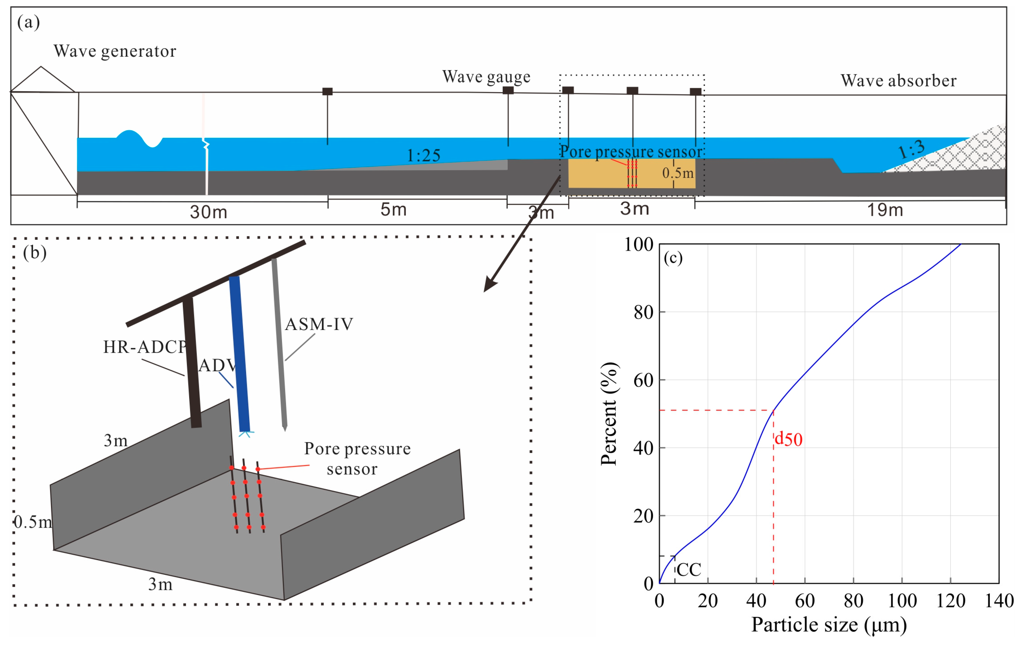
2.1. Experimental Flume and Instruments

Figure 1a shows a longitudinal section of the experimental flume. The flume was 60 m long, 3 m wide, and 1.5 m high. A piston-type hydraulic wave generator was located at one end of the experimental flume. A wave absorber was positioned at the opposite end (a porous plastic wave dissipation zone with a slope ratio of 1:3) to dissipate the incoming waves and minimize the reflected waves. A 1:25 slope was constructed 30 m from the wave generator to simulate the submarine slope beyond the coastal area. A soil tank (3 m long and wide, and 0.5 m deep) was located 38 m from the wave generator, with a transitional zone (3 m long and wide) between the slope and the soil tank.

Five wave gauges were used to record wave conditions. Each gauge had a precision of 0.001 m and a sampling rate of 50 Hz. The wave gauges were installed at the foot of the slope, top of the slope, left edge of the soil tank, middle of the soil tank, and the right edge of the soil tank, respectively (Figure 1a). Pore pressure was measured using 15 pore pressure sensors installed at 5 depths on a fixed frame along the centerline of the soil tank (z = 5, 10, 15, 30, and 45 cm, where z is the depth from the soil surface) (Figure 1b). The pore pressure sensors were capable of measurements between 0 and 10 kPa, with an accuracy of 0.05 kPa. These sensors were located on the same vertical plane as the wave gauge in the middle of the soil tank. During the experiment, the water flow velocity was obtained by an Aquadopp High-Resolution Profiler (HR-ADCP) with a measurement range from the bottom bed upward to 10 cm below the probe height (instrument blind area). The sampling frequency was 1 Hz and the layer size was 1 cm. An Acoustic Doppler Velocimeter (ADV) was used to measure the turbulence of the offshore bed (2 cm above the seabed) with a sampling frequency set at 32 Hz. An Argus Surface Meter IV (ASM-IV) turbidimeter was used to obtain the SSC data with high temporal and spatial resolution. The ASM-IV acquisition frequency was 1 Hz, the measurement range was from the bottom bed to the water surface, and the layer size was 1 cm. The spacing between HR-ADCP, ADV, and ASM-IV was 80 cm. To ensure the reliability of the experimental data, each sensor was calibrated in a simulated experimental environment prior to the study experiments.

Table 1. Parameters of the measuring instruments used in our experiments.

Instrument	Model	Sampling Rate	Precision	Range of Measurement
Pore pressure sensor	CYY2 piezoresistive sensor	16 Hz	0.5%	0–10 kPa
Wave gauge	Rod-shaped capacitive wave height gauge	50 Hz	0.2%	0.5–50.0 cm
Current meter	HR-ADCP	1 Hz	1%	1–25 cm
	ADV	32 Hz	0.5%	2 cm above the seabed
Turbidity profiler	ASM-IV	1 Hz	1%	1–96 cm

lists the parameters of the pore pressure sensors, wave gauges, HR-ADCP, ADV, and ASM-IV.

2.2. Soil Parameters

The experimental soils were obtained from a tidal flat near the mouth of the Yellow River. The main clastic minerals found in sediment samples were quartz, feldspar, calcite, and dolomite [13]. To ensure repeatability in successive experiments, these soils were dried, crushed, and passed through a sieve (with a sieve diameter of 0.4 mm) to remove all gravel impurities, then mixed with water, and finally thoroughly stirred to form remolded silt. The processed soils were then discharged into the soil tank until some excess slurry volume was maintained above the tank to ensure there was sufficient sludge sediment to completely fill the tank. Figure 1c presents the particle size distribution curve of the experimental soils. The experimental soil had a median particle size (d₅₀) of 46.5 μm. This shows that there was a large number of fine particles in the experiment soil, meaning it had low permeability and was apt to liquefaction [16,17].

2.3. Experimental Wave Conditions and Procedures

A series of random waves with different effective wave heights and average wave periods were generated according to the conventional JONSWAP (Joint North Sea Wave Project) spectrum.

Table 2. Experimental wave conditions.

Wave Condition	H (cm)	T (s)	D (cm)	Seabed Response
I-1	14	1.5	50	No liquefaction
I-2	14	2.0	50	No liquefaction
I-3	14	2.2	50	No liquefaction
I-4	14	2.5	50	No liquefaction
II-1	10	2.0	50	No liquefaction
II-2	14	2.0	50	No liquefaction
II-3	16	2.0	50	No liquefaction
II-4	18	2.0	50	No liquefaction
III-1	14	2.0	55	No liquefaction
III-2	14	2.0	50	No liquefaction
III-3	14	2.0	45	No liquefaction
III-4	14	2.0	40	No liquefaction
IV-1	14	2.0	50	Liquefaction
IV-2	16	2.0	50	Liquefaction
IV-3	18	2.0	50	Liquefaction
IV-4	18	2.0	50	Liquefaction

Note: H is the effective wave height; T is the average wave period; D is the water depth. For experiments I–III, the soil was settled for 48 h to allow consolidation, and then was placed under cyclic loading with a small-amplitude wave with H = 5 cm and T = 0.8 s to accelerate the consolidation process until the pore water pressure was stable; for experiment IV, the soil was consolidated for 12 h in a static environment.

lists the experimental wave conditions. The duration of wave action in each experiment was 1200 s, with four distinct wave conditions (I, II, III, and IV). We performed 16 experiments. Each experiment was labeled according to the wave condition and experimental number for that specific condition (e.g., II-3 refers to the third experiment at wave condition II). First, the flume and soil tanks were cleaned, followed by installation of the pore pressure sensors, wave gauges, HR-ADCP, ADV, and ASM-IV (which had been prepared by soaking them in water) at their designated positions. The experimental soil was then mixed in water and transferred into the soil tank. After self-consolidation for 48 h, the flume was filled to the designed water level. A small wave height of 5 cm and period of 0.08 s was used to accelerate soil consolidation until the pore pressure stabilized at all depths. This step ensured the proper degassing of the seabed, which reduced the porosity, increased the soil strength, and improved the overall uniformity of the soil characteristics. Finally, waves were generated according to the designed wave conditions as described in Table 2. Concurrently, the experimental process was recorded by video.

2.4. Data Processing

2.4.1. Soil Liquefaction Criteria

Under the wave load, the increase in excess pore pressure is an important index to indicate the change in soil state. The change of cumulative pore pressure caused by the accumulation of excess pore pressure can be used to judge whether the soil is under liquefaction [7].

The excess pore pressure at a certain depth is described by Equation (1):

$$P=P_m-P_w$$

(1)

where $P$ is the excess pore pressure (unit: Pa); $P_m$ is the measured pore pressure (unit: Pa); and$P_{w }$is the static pore pressure (unit: Pa).

The cumulative excess pore pressure is described by Equation (2) [18]:

$$\overline{P}=\frac{1}{T}{{\displaystyle \int }}_t^{t+T}Pdt$$

(2)

where $\overline{P}$ is cumulative excess pore pressure (period-averaged excess pore pressure, unit: Pa), T is the average wave period (unit: s), and $t$ is the run time of the experiments (unit: s).

The initial mean normal effective stress of the soil under static water conditions is described by Equation (3) (${\sigma }_0$, unit: Pa or N/m²) [18]:

$${\sigma }_0={\mathsf{ϓ}}^{\prime }z\frac{1+2k_0}{3}$$

(3)

where k₀ is the static lateral earth pressure coefficient, representing the ratio between horizontal and vertical effective stress (k₀ is not a constant value for silt) which was set at 0.57 for these experiments; $z$ is the depth from the soil surface; and ${\mathsf{ϓ}}^{\prime }={\mathsf{ϓ}}_s-{\mathsf{ϓ}}_w={\rho }^{\prime }g$ is the submerged unit weight of the test soil, $g$ is the gravitational acceleration, ${\rho }^{\prime }$ is the effective density of soil, which is defined as the density of soil minus the density of water. So, ${\mathsf{ϓ}}^{\prime }$ is related to water content and saturation degree [19]. The measured initial submerged unit weight ${\mathsf{ϓ}}^{\prime }$ of the test soil in experiments I, II, III, and IV before the wave action is 8.85, 8.46, 8.32, and 5.46 kN/m³, respectively. It should be mentioned that the submerged unit weight of the test soil changed during the wave action process, but we did not sample the test soil and measure the ${\mathsf{ϓ}}^{\prime }$ value during the experiments to avoid the artificial disturbance to the test soil, so we used the initial measured ${\mathsf{ϓ}}^{\prime }$ values for calculating the initial mean normal effective stress ${\sigma }_0$.

Several criteria were proposed for discriminating liquefaction [19], most of which are based on effective normal stress or excess pore pressure. Jeng [20] proved that the optimal criteria for identifying soil liquefaction in laboratory experiments with shallow thickness of testing soil is to compare the excess pore pressure to the initial average normal effective stress. Based on this criterion, liquefaction occurs when the cumulative excess pore pressure ($\overline{P}$) reaches the initial mean normal effective stress (${\sigma }_0$) [18,21].

$${\sigma }_0\le \overline{P}$$

(4)

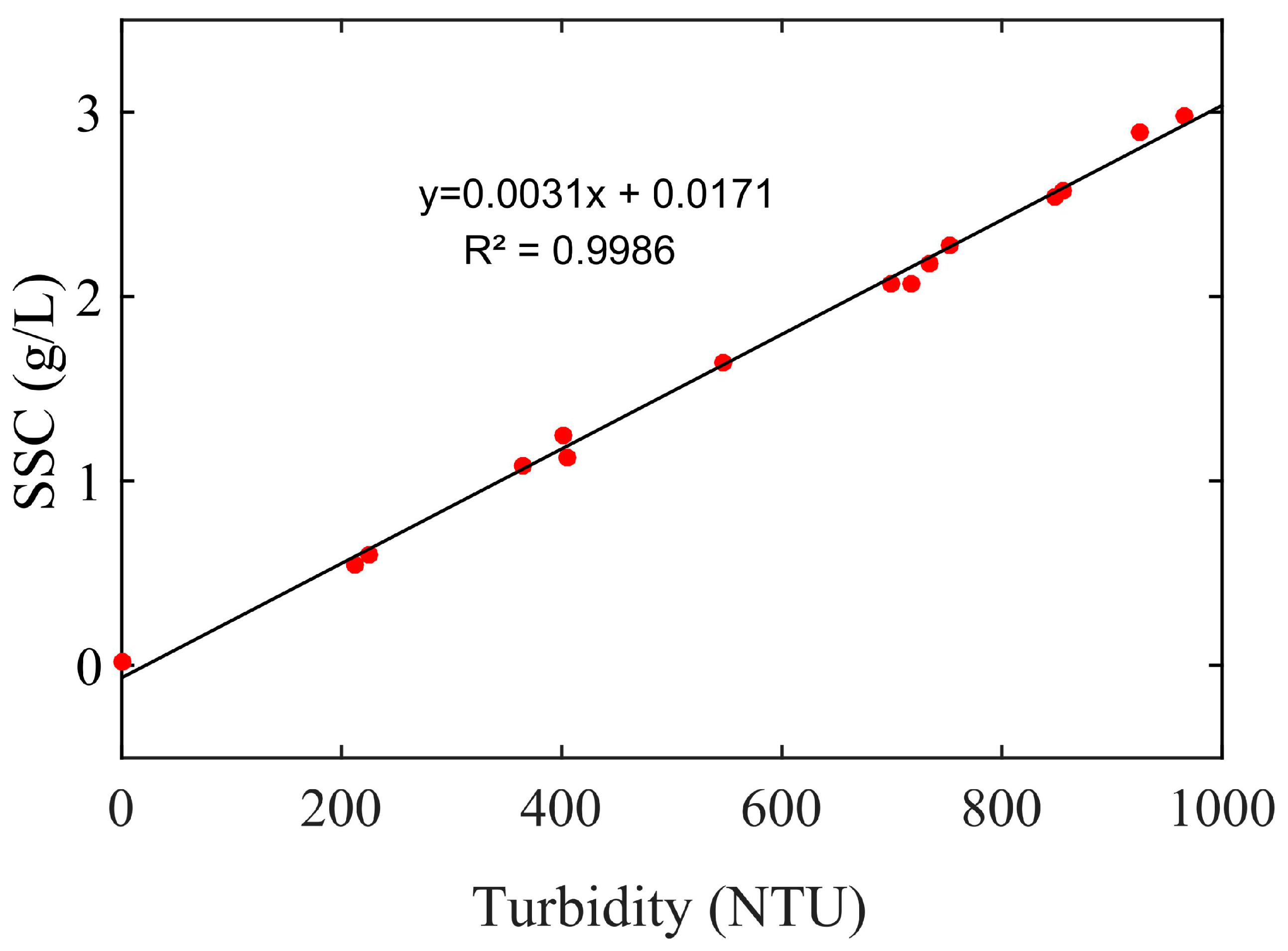
2.4.2. Method for CALCULATING SSC

The spatial and temporal changes of SSC in the water column were recorded via the ASM-IV. The ASM-IV records the reflections and the dynamic parameters that are created in a water column by solid particles moving in a multiphase current, and responds directly to SSC. Therefore, it may be used to identify process-driven variations in water turbidity. The conversion from turbidity-to-SSC values has been achieved through laboratory calibration. Further descriptions of the calibration methodology can be found in Hu et al. [22]. The turbidity-to-SSC conversion formula was deduced via linear regression (Figure 2), as shown in Equation (5):

$$y=0.0031x+0.0171$$

(5)

where x is the turbidity (NTU), and y is SSC (unit: g/L). An R² of 0.9986 indicates that the conversion was reliable enough to accurately estimate the SSC.

2.4.3. Method for Calculating Wave Shear Stress

The wave shear stress (${\tau }_w$, unit: Pa or N/m²) is described in Equations (6)–(8) [23]:

$${\tau }_w=\frac{1}{2}\rho f_w{U}_w^2$$

(6)

$$U_w^2=\frac{0.5\mathrm{H}\mathsf{\omega }}{\sin \mathrm{h}\left(\mathrm{kD}\right)}$$

(7)

$$f_w=\exp \left[-6+5.2{\left(\frac{A_{\delta }}{k_s}\right)}^{-0.19}\right]$$

(8)

where $\rho$ is the water density, $U_w$ is the near-bottom wave orbital velocity, f_w is the wave friction factor, $\omega =\frac{2\pi }{T}$ is the angular or radian frequency,$k=\frac{2\pi }{L}$ is the wave number, $k_s=\frac{2.5d_{50}}{30}$ is the bottom physical roughness, and $A_{\delta }=\frac{U_{w}T}{2\pi }$ is the near-bottom excursion amplitude.

2.4.4. Method for Calculating Turbulent Kinetic Energy (TKE)

The ADV measured bottom boundary-layer velocity, including the longitudinal (along the flume) component 𝑢, transverse component 𝑣, and vertical component 𝑤, and is composed of average velocity and fluctuating velocity. That is:

$$v=\overline{v}+\left(v_t^{\text{'}}+v_w^{\text{'}}\right)$$

(9)

where $\overline{v}$ is the temporal mean velocity, and $v_t^{\text{'}}$ and $v_w^{\text{'}}$ are the velocities of the turbulent component and wave component, respectively [24,25]. To understand the impact of turbulence and wave energy on seabed surface sediments, it is necessary to decompose the turbulent and wave components in the fluctuating velocity.

In this study, we used a Synchrosqueezed Wavelet Transform (SWT)-based method for wave-turbulence decomposition. Previous studies have confirmed the advantages and effects of SWT in wave-turbulence decomposition [24,25]. After decomposing the turbulent and wave components, $TKE$(unit: m²/s²) is described by Equation (10) [26]:

$$TKE=\frac{1}{2}\left(u_t^{\text{'}}{}^2+v_t^{\text{'}}{}^2+w_t^{\text{'}}{}^2\right)$$

(10)

3. Experimental Results

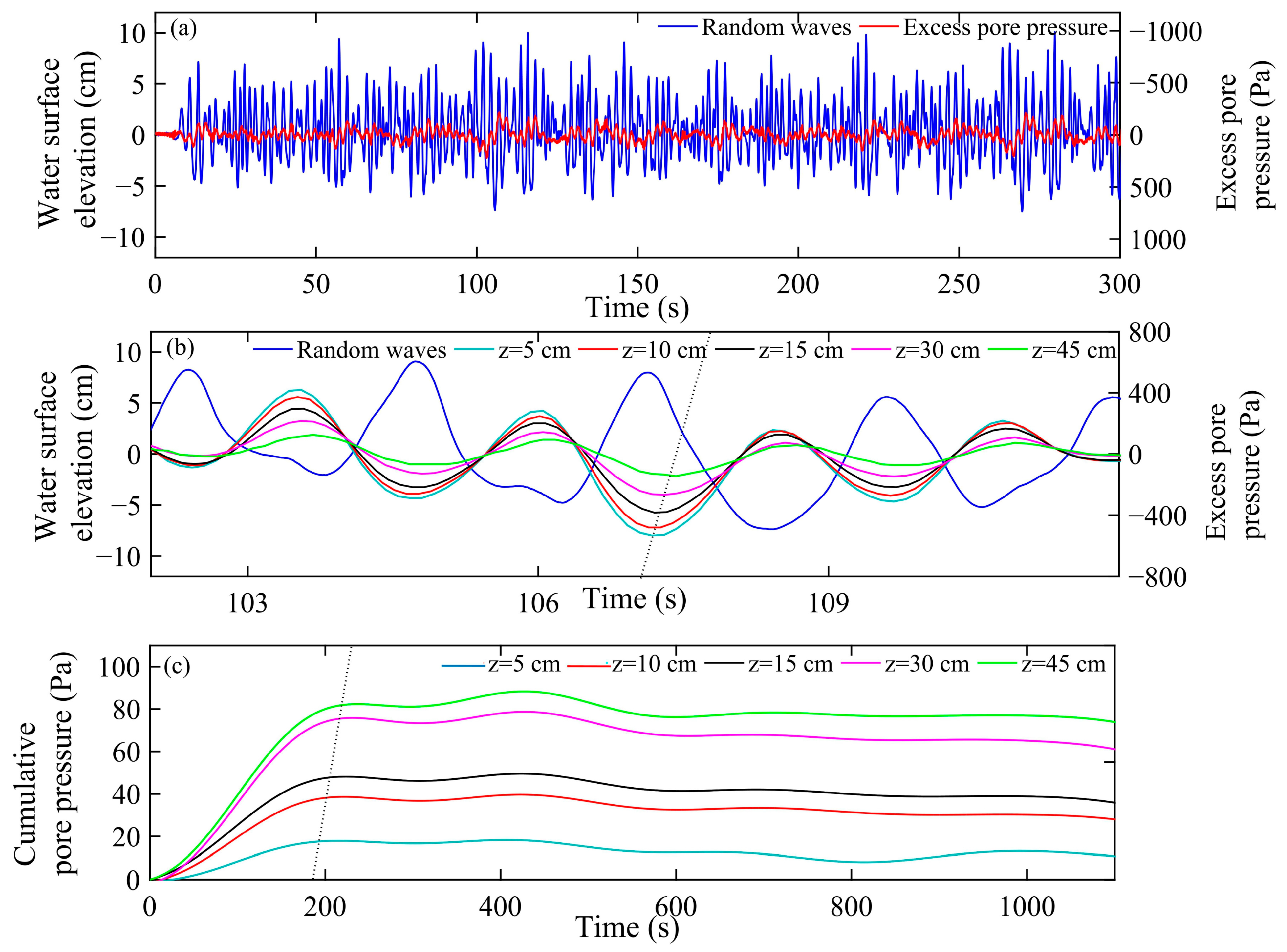
3.1. Excess Pore Pressure Response to Random Waves in Nonliquefied Soil

Figure 3 shows the time-series of the random wave in experiment I-2, the corresponding excess pore pressures at 10 cm, and cumulative pore pressure during the experimental process. Figure 3a shows the excess pore pressure response at a soil depth of 10 cm to the random wave. It shows that the trend of excess pore pressure amplitude changes corresponded with the trend of random waves. Figure 3b shows the change of excess pore pressure response at different depths of the seabed with time and indicates that the amplitude of excess pore pressure decreased as depth increased. Additionally, there was a clear time lag between the excess pore pressure of each layer at distinct depths. The waveform phase of excess pore pressure was opposite from that of the random waves. The excess pore pressure waveforms reached a minimum at the crests of the random waves and a maximum at the troughs. This was consistent with what Zen and Yamazaki [27] and Xu et al. [28] observed in the field. This occurs because, as the wave-induced hydrodynamic pressure generated randomly is transmitted to the deep seabed, seabed soil particles are compressed and elastically deformed, extruding soil particles and increasing excess pore pressure. As the water surface drops from the crest, the total pressure inside the seabed decreases, restoring the elasticity of the soil particles, decreasing their pressure and the excess pore pressure. After the trough, the pressure on soil particles and the excess pore pressure increases again, with the changes in excess pore pressure constantly lagging that of the random waves. Figure 3b shows selected typical excess pore pressure periods (Figure 3b, dashed-line section). As can be seen from the excess pore pressure response at different depths, the lag of excess pore pressure fluctuation increased as the depth below the seabed increased. For each additional 10 cm of depth, the time lag was about 0.125 s. This trend was the same as Song et al. [29] observed in situ at the Chengdao oilfield. Figure 3c shows the cumulative pore pressure over time at each depth. In the figure, the various colored lines represent different depths and the dashed line denotes the time required to reach the first crest at distinct depths. Figure 3c shows that excess pore pressure accumulation occurred in all depths, and the cumulative pore pressure increased as the depth increased. Impacted by waves, excess pore pressure started to accumulate at each depth. The cumulative pore pressure at a depth of 5 cm reached a crest at t = 185 s, followed by z = 10, 15, 30, and 45 cm at t = 190, 194, 197, and 202 s, respectively. The maximum cumulative pore pressure for each layer was 18.5, 49, 59, 78, and 89 Pa, respectively. All recorded pressures were lower than their corresponding ${\sigma }_0$ at 302, 604, 906, 1812, and 2718 Pa, respectively, and accounted for less than 7% of the theoretical ${\sigma }_0$. Based on this, the soil did liquefy in this experiment, but there was an upward pressure gradient on the seabed which was sustained until the end of the wave impact.

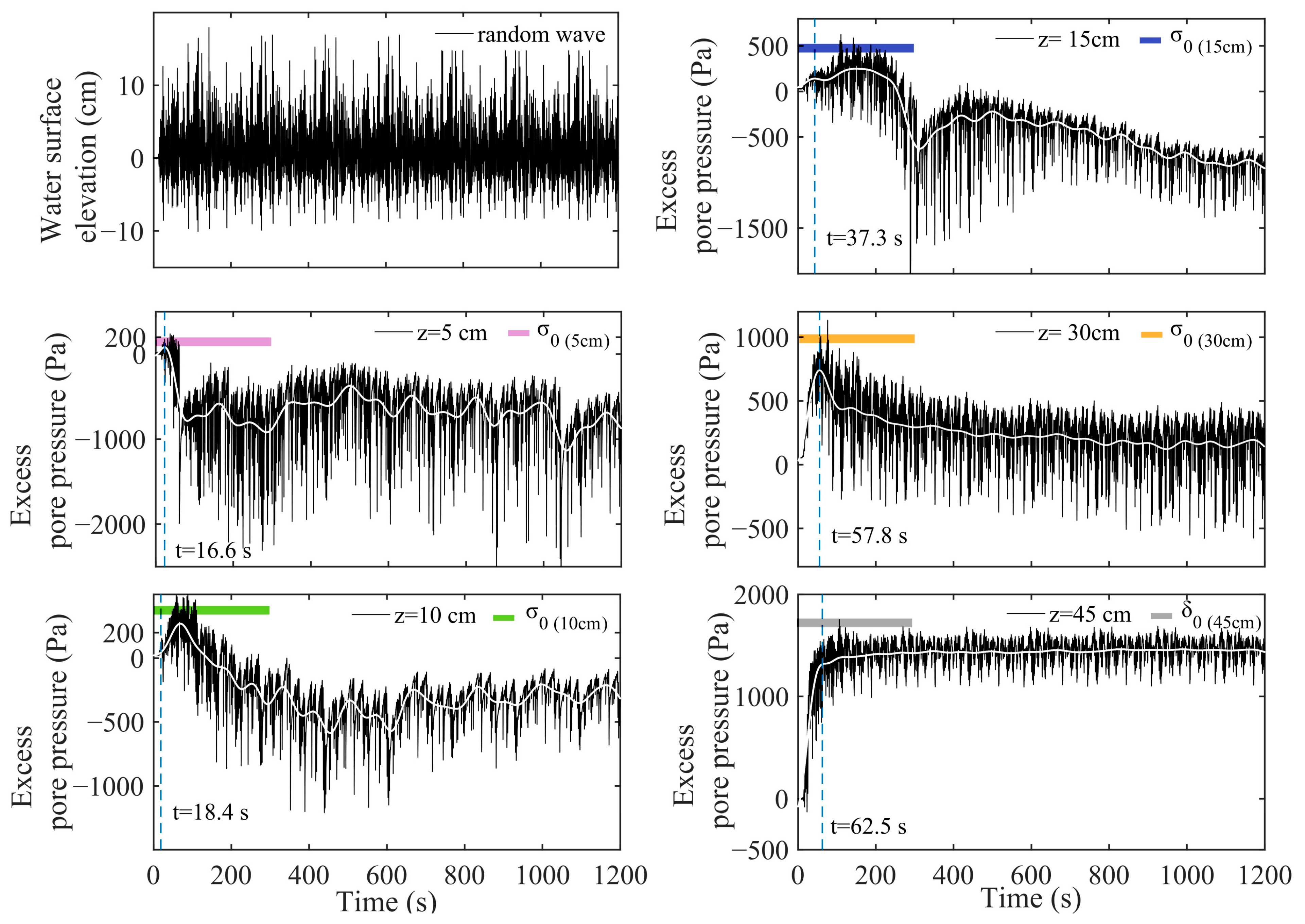
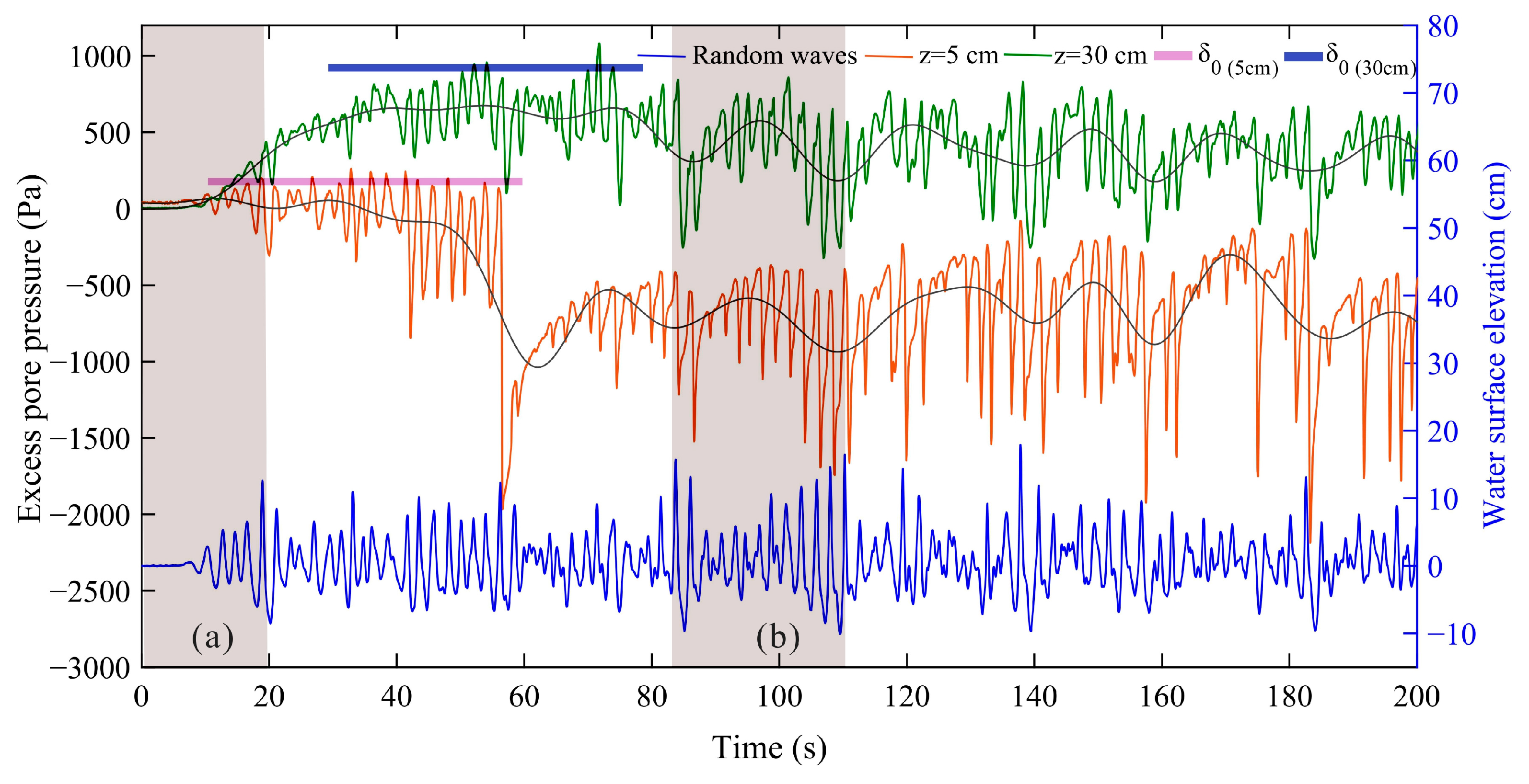
3.2. Excess Pore Pressure Response to Random Waves in Liquefied Soil

This section discusses the soil excess pore pressure response characteristics in the liquid state. Experiment IV was conducted following 12 h of natural consolidation within the soil bed. Figure 4 shows that at the beginning stage of wave impact, soil layers experienced excess pore pressure accumulation. Cumulative pore pressure increased with depth. Excess pore pressure accumulated rapidly at z = 5 cm below the surface of the seabed, reaching the first crest of cumulative pore pressure at t = 16.6 s. At t = 61 s, excess pore pressure decreased drastically to negative, indicating that the soil suddenly liquefied, destroying its honeycomb structure. Particles of the soil framework experienced relative displacement, porewater between particles was released, resulting in negative excess pore pressure. Liu et al. [30] also observed negative excess pore pressure through field experiments and believed that it was caused by dilation effects after the sediment was damaged, which was related to soil liquefication. During the field monitoring at the Yellow River Delta, scholars also reported negative excess pore pressure during soil liquefaction and submarine landslides caused by storm waves [31]. At z = 10 cm and z = 15 cm below the surface of the seabed, changes in excess pore pressure were similar to those at z = 5 cm. At the initial stage of wave impact, excess pore pressure accumulated continuously in the seabed, reaching a crest at t = 18.4 s and t = 37.3 s, respectively. When the cumulative pore pressure of the seabed approached ${\sigma }_0$, excess pore pressure decreased rapidly to negative.

However, the z = 30 cm layer had a different excess pore pressure fluctuation pattern from the layer above. Although excess pore pressure also accumulated continuously at the initial stage of wave impact, when it crested (t = 57.8 s), it did not plummet to negative, but slowly dissipated. This was because porewater between soil particles was drained after soil liquefaction, compressing the seabed and rearranging soil particles, making the soil more compact. Therefore, there was no re-accumulation of excess pore pressure. Excess pore pressure also accumulated rapidly at z = 45 cm during the initial stage of wave impact. It approached the first crest at t = 73 s, then remained nearly constant for the next 1100 s. However, the momentary pore pressure fluctuated in response to wave oscillation. This indicates that the soil framework deformed at this depth but did not liquefy. From the analysis above, we conclude that during the initial stage of wave impact, excess pore pressure accumulated continuously in the seabed, and the cumulative pore pressure increased with depth. It was the lowest in the shallow sediments (Figure 4), forming an upward pressure gradient. When excess pore pressure reached the ${\sigma }_0$ of the soil, the seabed liquefied, forming a liquefaction zone in the top layers and then extending downwards. This result is consistent with those reported by Jia et al. [12].

Figure 5 shows the detailed variation characteristics of the excess pore pressure response of the liquefied seabed under the action of random waves. The response of excess pore pressure in the liquefied state (shaded area b in Figure 5) remained consistent with the changing trend of waves. However, there were clear abrupt changes in the fluctuation pattern, which demonstrated asymmetric crests and troughs, having flatter crests and sharper troughs. This was notably different from the wave characteristics in the nonliquefied state (Figure 3b). In particular, the excess pore pressure response in the liquefied state was negative because the seabed consolidation time was short, and initial pore pressure had not completely dissipated. Therefore, the initial pore pressure of the seabed was high while ${\sigma }_0$ was low. After liquefaction, porewater was drained, causing excess pore pressure to drop below the initial pressure.

In addition, the shaded areas (a) and (b) in Figure 5 also show the difference in excess pore pressure response between nonliquefied (a) and liquefied (b) seabed impacted by random waves. Shaded area (a) shows the initial stage of wave impact when the seabed was in a nonliquefied state. The excess pore pressure accumulated as the amplitude of the waves increased. Shaded area (b) shows the excess pore pressure response of the liquefied seabed. Large-amplitude waves dissipated excess pore pressure in liquefied soil, while the pressure increased with small-amplitude waves. Additionally, under the same wave conditions, the amplitude of excess pore pressure response was larger for soil in the liquefied state than in the nonliquefied state.

In this experiment, the most notable characteristic of the liquefied seabed was that the soil was moving elliptically with the waves, forming mud waves. This phenomenon was also observed by Wen et al. [32], Jia et al. [12], and Sumer et al. [18]. Jia et al. [12] regarded the oscillation of seabed sediment as a sign of seabed liquefaction, but other scholars believed that it was caused by wave-induced ${\tau }_w$exceeding the shear stress of the seabed [33]. We believe that the formation of mud waves was the result of both the accumulation of excess pore pressure caused by waves and ${\tau }_w$. Figure 6 shows the progressive change at the seabed interface during a single wave cycle. The seabed mud wave fluctuated in phase with the wave. This means that the crests and troughs of the mud wave coincided with the crests and troughs of the wave. To further study the pattern of mud-wave motion with the wave, Matlab (version Matlab 9.10, Developed by the MathWorks Inc. in the United States) was used to extract the position of the yellow line in Figure 6a, frame-by-frame from the video recording, to depict the fluctuation of the seabed interface. Figure 7 shows the fluctuation of the mud wave through time as it fluctuated with the wave. In Figure 7, the blue curve represents the curve of the random waves through time and the black curve represents the fluctuation of the mud waves. The amplitude of the mud wave gradually increased as wave impacts continued. This means that the amplitude of the mud wave gradually increased as liquefication extended deeper into the seabed. The amplitude of the mud wave increased from 1–2 cm at the beginning of liquefaction to 5–6 cm at the maximum. Considering the typical short-term process shown in Figure 7, larger-amplitude mud waves corresponded to larger-amplitude water waves, and smaller-amplitude mud waves corresponded to smaller-amplitude water waves. After seabed liquefaction, the soil on the seabed fluctuated together with the waves, resulting in differing stresses on the soil at the crests and troughs of the waves. This led to sharper troughs and flatter crests for the seabed excess pore pressure waveform.

Impacted by waves, the seabed–soil structure was destroyed, and the seabed liquefied, substantially altering the oscillation waveform of excess pore pressure as it plummeted to negative. Concurrently, once the seabed was liquefied, its interface began to move elliptically with the waves, forming mud waves. The amplitude of the mud waves increased as the depth and degree of liquefaction increased. Therefore, this study indicates that the excess pore pressure “plummeting to negative” and the “elliptical motion of mud waves” can be used as an indicator of seabed–soil liquefaction.

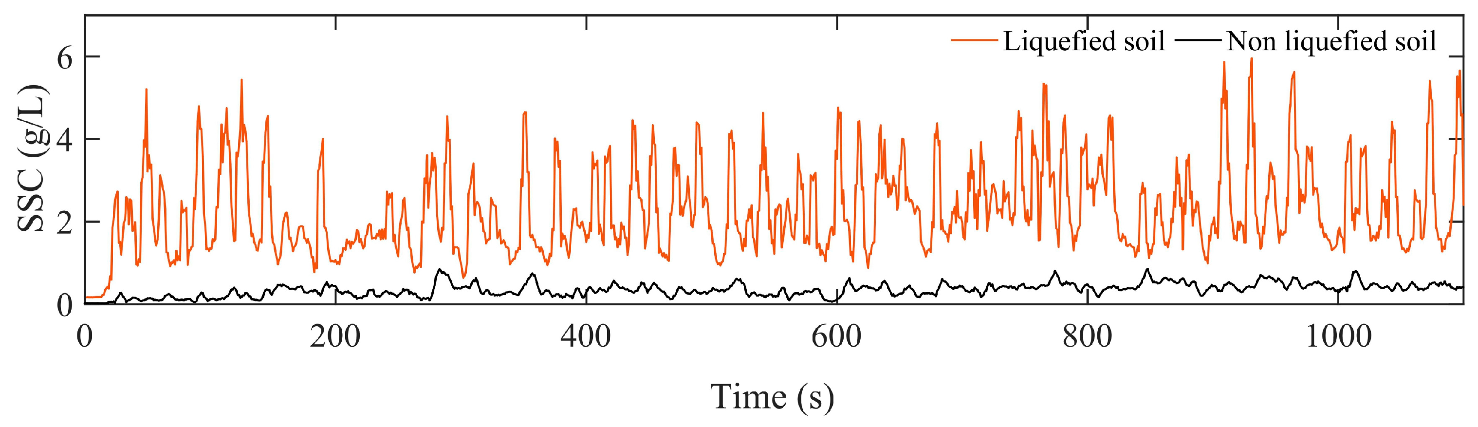
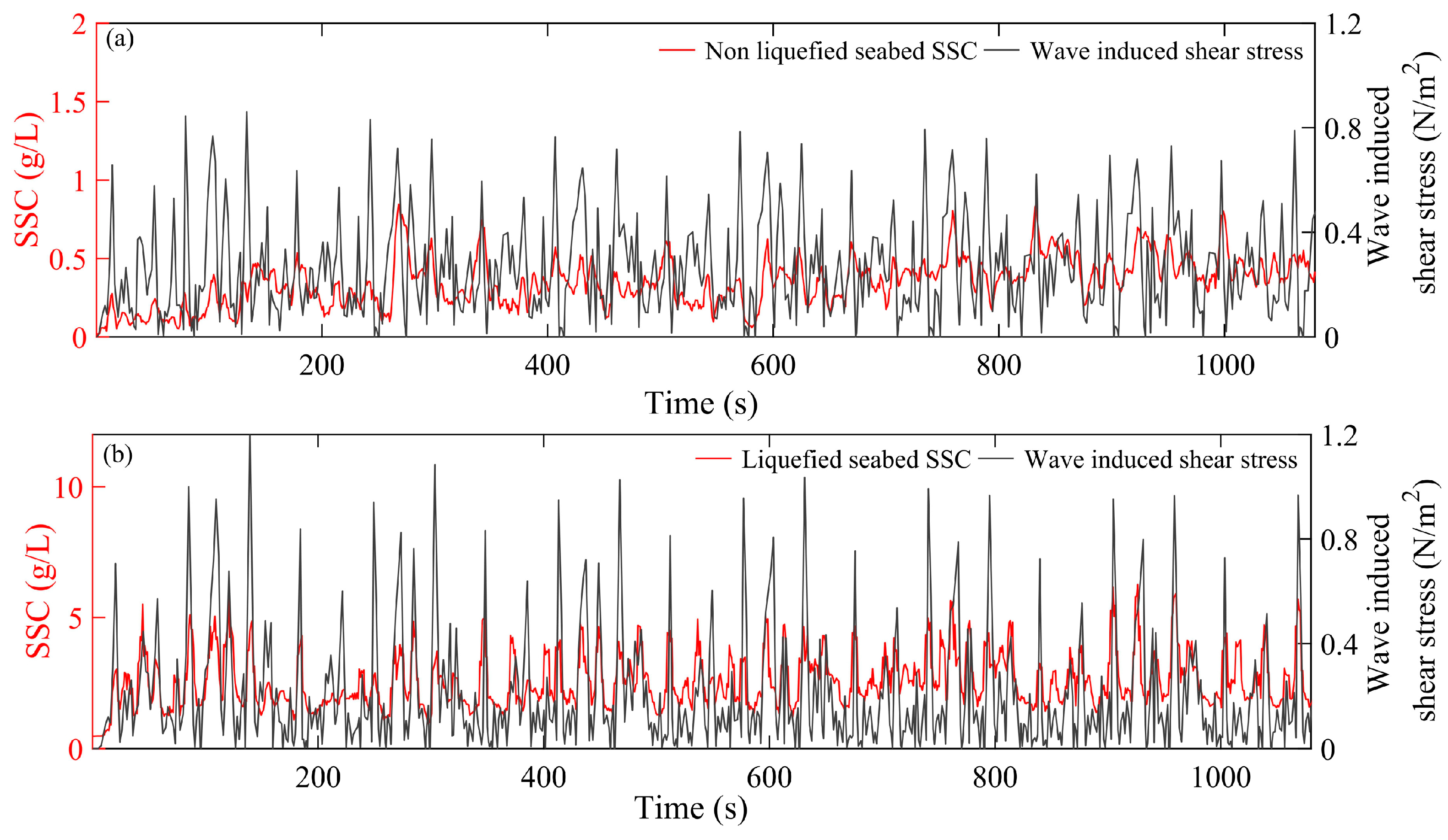
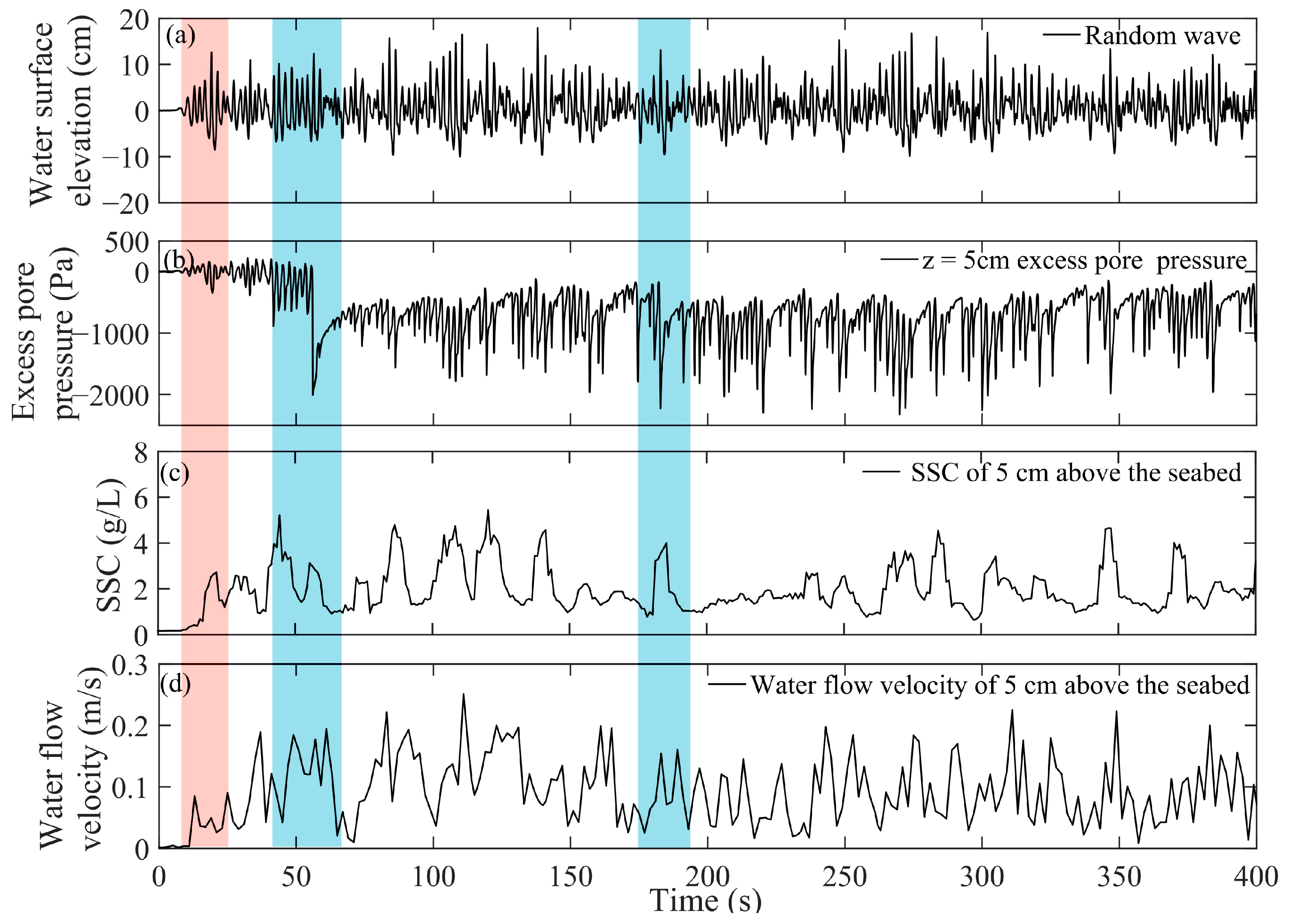
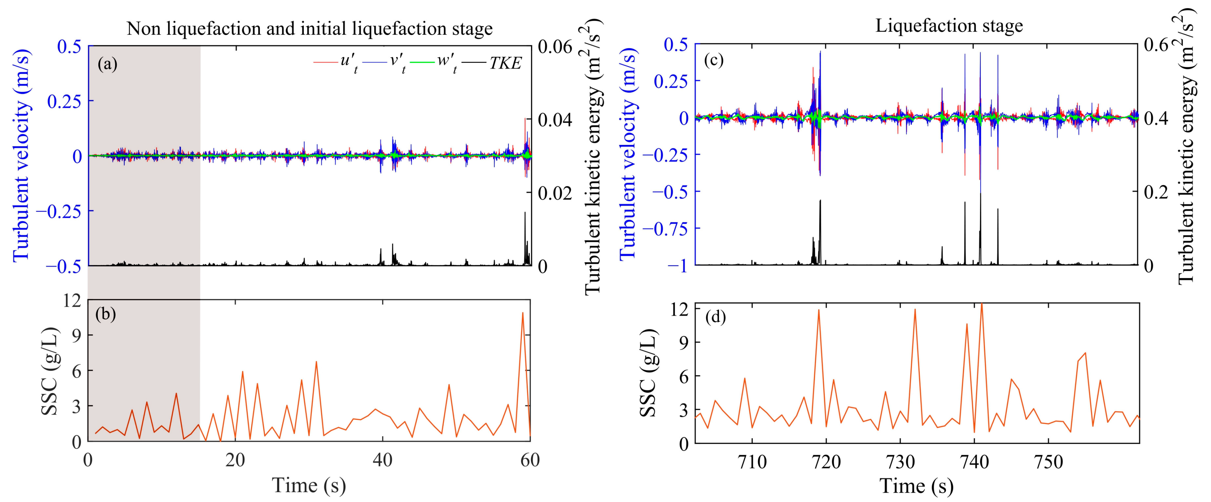
3.3. Sediment Resuspension Induced by Random Waves

Figure 8 shows SSC changes of nonliquefied and liquefied soil. Figure 8a,b represent the nonliquefied state and Figure 8c,d represent the liquefied state. Figure 8a,c depict an effective wave height of 16 cm. Figure 8b,d correspond to an effective wave height of 18 cm. In the initial stage of wave impact, the SSC of bottom water increased rapidly and gradually expanded upwards. As the wave impact continued, the SSC of bottom water gradually increased and showed a pattern of “higher on the bottom and lower on the top.” A comparison of the seabed in a nonliquefied and liquefied state under similar wave conditions (e.g., Figure 8a,c) reveals that the SSC in the liquefied state was much greater than that in the nonliquefied state.

To further analyze the detailed change in SSC in the nonliquefied and liquefied state, Figure 9 shows the SSC change at 5 cm above the seabed under the same wave conditions (experiments II-3 and IV-2). The bottom layer SSC of the nonliquefied seabed started to increase at t = 14 s, reached the first crest of 0.27 g/L at t = 28 s, and its maximum of 0.85 g/L at t = 844 s. The overall trend of SSC was an increase with fluctuations caused by changes in ${\tau }_w$. The increase of SSC at this stage was chiefly owing to the resuspension of surface sediments, which corresponds with the observations of Zhang et al. [14]. For the liquefied seabed, the bottom layer SSC started to increase at t = 9 s and reached the first crest of 2.72 g/L, 10 times the concentration of the nonliquefied seabed, at t = 21 s. During this process, the soil near the surface was liquefied (Figure 9). Then, SSC increased substantially at approximately t = 40 s, caused by the liquefaction of the 15 cm-deep seabed (Figure 9). At t = 926 s, SSC reached its maximum of 5.95 g/L. These results indicate that the liquefied seabed had a much higher SSC than the nonliquefied seabed, with the maximum of the former at seven times that of the latter.

4. Discussion

Experimental results show that the SSC above the liquefied seabed was 7–10 times higher than that above the nonliquefied seabed. This indicates that soil liquefaction may play a key role in the sediment resuspension process. To further examine the effect of seabed liquefaction on sediment suspension, the relationship between the bottom layer SSC and ${\tau }_w$ during the experiments of wave conditions II-3 (nonliquefaction) and IV-2 (liquefaction) is shown in Figure 10. Changes in water surface fluctuation, seabed excess pore pressure, near-bottom flow velocity, and SSC during the experiment of wave condition IV-2 (liquefaction) are shown in Figure 11.

Figure 10 indicates that the measured SSC on nonliquefied and liquefied seabed were both closely related to ${\tau }_w$, as SCC increased with ${\tau }_w$. For the nonliquefied seabed, in the initial stage of wave impact, the waves and currents drove the sediment particles into a suspended state, and the SSC in the water body increased slightly. Subsequently, the suspended state of the sediment particles depended on the support of the turbulent water body. If there was a decrease in current velocity and wave height, SSC would have decreased. With the continuous impact of waves, an upward pressure gradient formed inside the seabed (Figure 3c). Owing to this pressure gradient, fine particles in the seabed were transferred upward along seepage channels and eventually suspended in the water, resulting in an increase of SSC (Figure 10a).

For the liquefied seabed, with short soil consolidation time, low ${\sigma }_0$, and the low shear resistance of the particles, liquefaction occurred rapidly in the shallow layers of the soil, owing to wave loading and the rapid accumulation of excess pore pressure in the seabed near the surface (the shaded area in Figure 5 and the red shaded area in Figure 11). The SSC of the seabed near the bottom of the water column increased rapidly, enhancing the hydrodynamic conditions, increasing the flow rate from the initial peak of 0.09 m/s to 0.19 m/s. This indicates that a substantial material exchange occurred near the seabed. With the continuous impact of waves, the degree of liquefaction of the seabed continued to increase in a regular pattern, along with the material exchange between the seabed and the water body. As the excess pore pressure dissipated (when porewater was drained), the SSC near the seabed increased, leading to a higher water flow velocity. When excess pore pressure accumulated, the SSC near the seabed decreased, and the measured water flow velocity was reduced (as shown in the blue shaded area in Figure 11). These results demonstrate that liquefaction of the seabed changes the sediment suspension in the water and causes substantial material exchange between the water and soil.

Concurrently, Figure 12 shows the relationship between turbulent flow velocity and TKE in different liquefaction stages and SSC. Figure 12a,b represent the stages of nonliquefaction and initial liquefaction. Figure 12c,d represent the later stages with a high degree of liquefaction. For the nonliquefied seabed, the turbulent flow velocity in all directions was small; u’_t and v’_t were similar, with a maximum of approximately 0.04 m/s; and the value of w’_t was small, with a maximum of approximately 0.01 m/s. TKE was also small, with a maximum of 0.0008 m²/s², which owed to the seabed being flat at the initial stage of wave impact. This planar surface was not conducive to the generation of turbulence, so the effect of turbulence on the seabed was small (shaded area in Figure 12a). With the continuous impact of waves, the seabed gradually liquefied, and its interface began to fluctuate with random waves. This was conducive to the generation of turbulence, and TKE gradually increased. When varying degrees of liquefaction occurred in all parts of the seabed (t = 60 s), u’_t and v’ increased to 0.16 m/s, w’_t increased to 0.03 m/s, and TKE increased to 0.015 m²/s². Owing to the increase of TKE, the turbulent shear of the seabed was enhanced, increasing the SSC to 10.9 g/L at 2 cm above the seabed (Figure 12a,b). As seabed liquefaction continued to increase, the vibration amplitude of the seabed interface also increased, leading to higher turbulent velocity and TKE. The values of u’_t and v’_t increased to 0.35 m/s (9 times that at the nonliquefied state), w’_t increased to 0.06 m/s (6 times that at the nonliquefied state), and TKE increased to 0.18 m²/s² (200 times that at the nonliquefied state). In this stage, turbulent waves had a more drastic impact on the seabed, increasing the SSC at 2 cm above the seabed to 11.9 g/L (Figure 12c,d).

As described above, liquefaction of the seabed leads to increases in SSC and water velocity. Here, the mechanism by which seabed liquefaction affects SSC is discussed (Figure 13). First, though ${\tau }_{w }$plays an important role in the resuspension of seabed surface sediments above both liquefied and nonliquefied seabeds (Figure 10), for a liquefied seabed, owing to excess pore pressure accumulation, the honeycomb structure of soil was destroyed, reducing the bonding between soil particles and the erosion resistance of seabed sediments. This resulted in the seabed being more prone to erosion under the same wave conditions. Second, because silty soil is a type of pigging soil, following seabed liquefaction and owing to the upward pressure gradient, the fine particles carried by porewater migrate to the surface of the seabed in seepage channels between coarse particles. Concurrently, following seabed liquefaction, the soil strength is lost, generating mud waves in elliptical motions along with random waves conducive to the generation of turbulence, increasing the TKE by several orders of magnitude. Turbulent shear and seepage also enhance the sediment resuspension. Furthermore, in the experiments, excess pore pressure dissipated as random waves crested, draining the pore water in the seabed. The discharged porewater carried copious amounts of sediment upward into the water body, resulting in an increase in SSC.

5. Conclusions

This study used a large-scale flume experiment to simultaneously observe the changes of pore pressure in the seabed and SSC near the seabed under the impact of random waves. Using real-time observation and video recording, the liquefaction characteristics of the silty seabed and the patterns of sediment resuspension were studied. The main conclusions are as follows:

(1)

The excess pore pressure in the nonliquefied seabed oscillated with wave fluctuations, but there was a net upward pressure gradient, which possibly promoted sediment resuspension.

(2)

After seabed liquefaction, there were abrupt changes in the waveforms of excess pore pressure, generating asymmetric crests and troughs with relatively flat crests and sharp troughs. Seabed liquefaction first occurred in the shallow layers, and expanded downward. Large-amplitude waves dissipated excess pore pressure and small-amplitude waves accumulated it. This response differed to that of the nonliquefaction state.

(3)

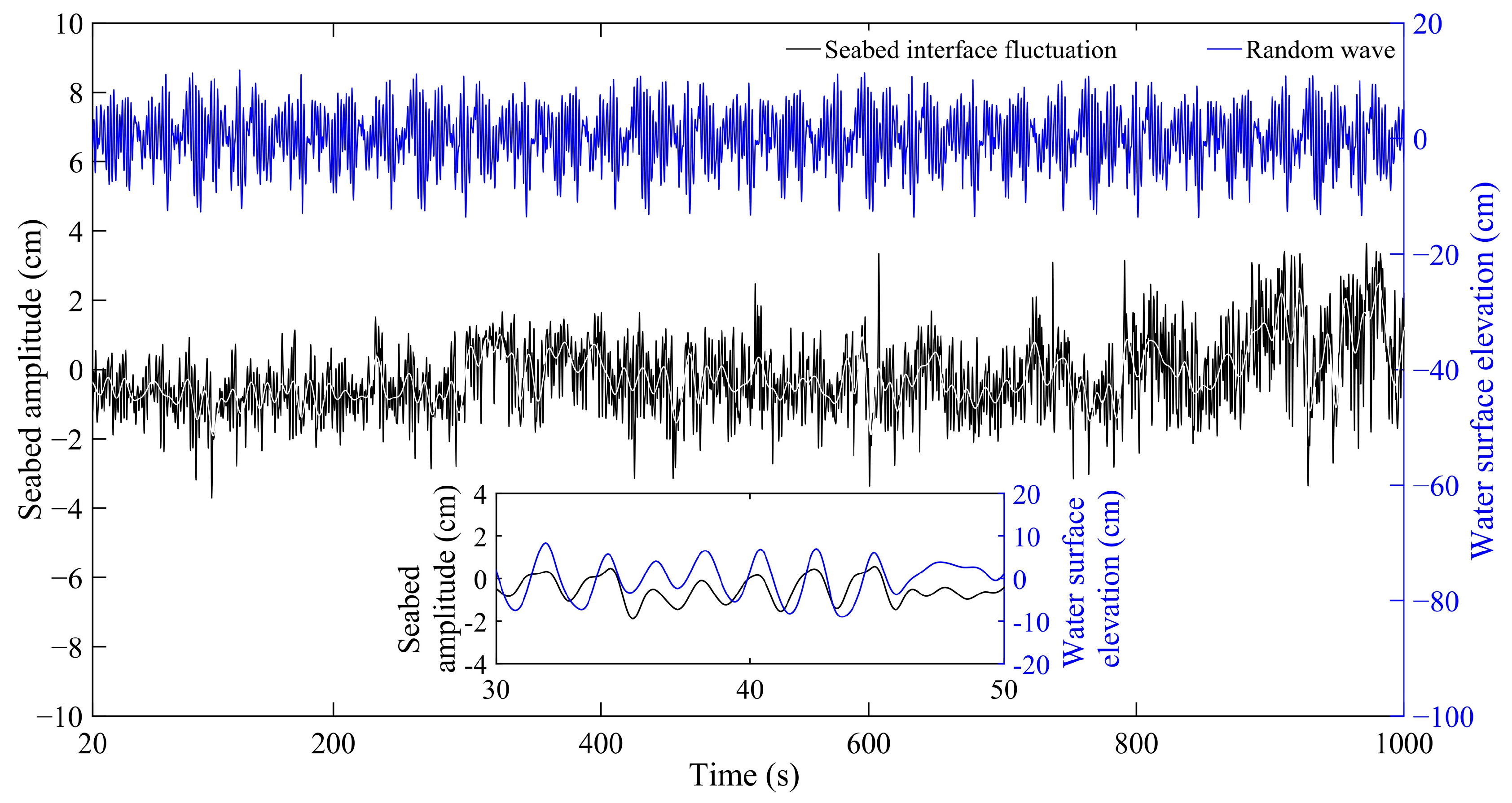
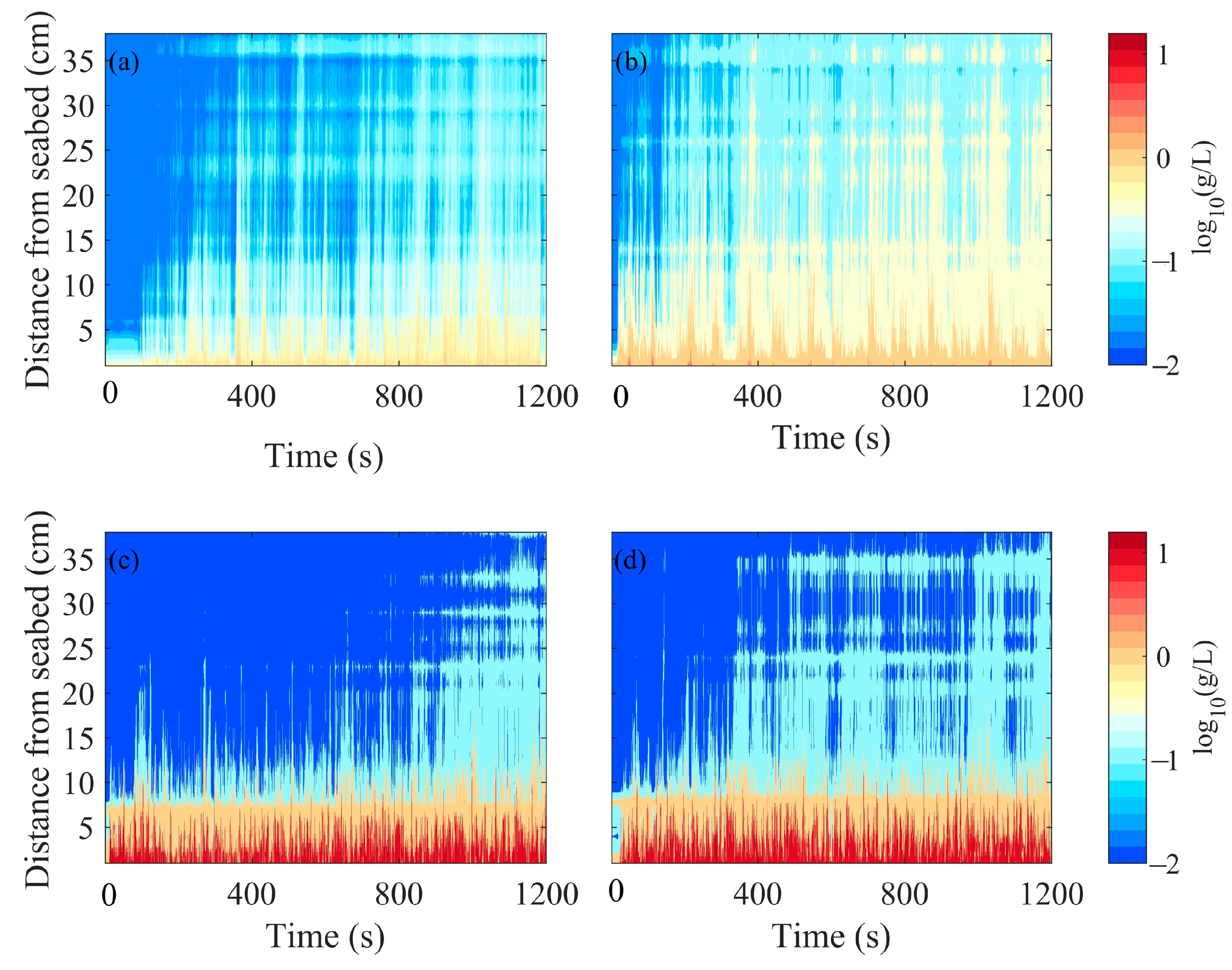
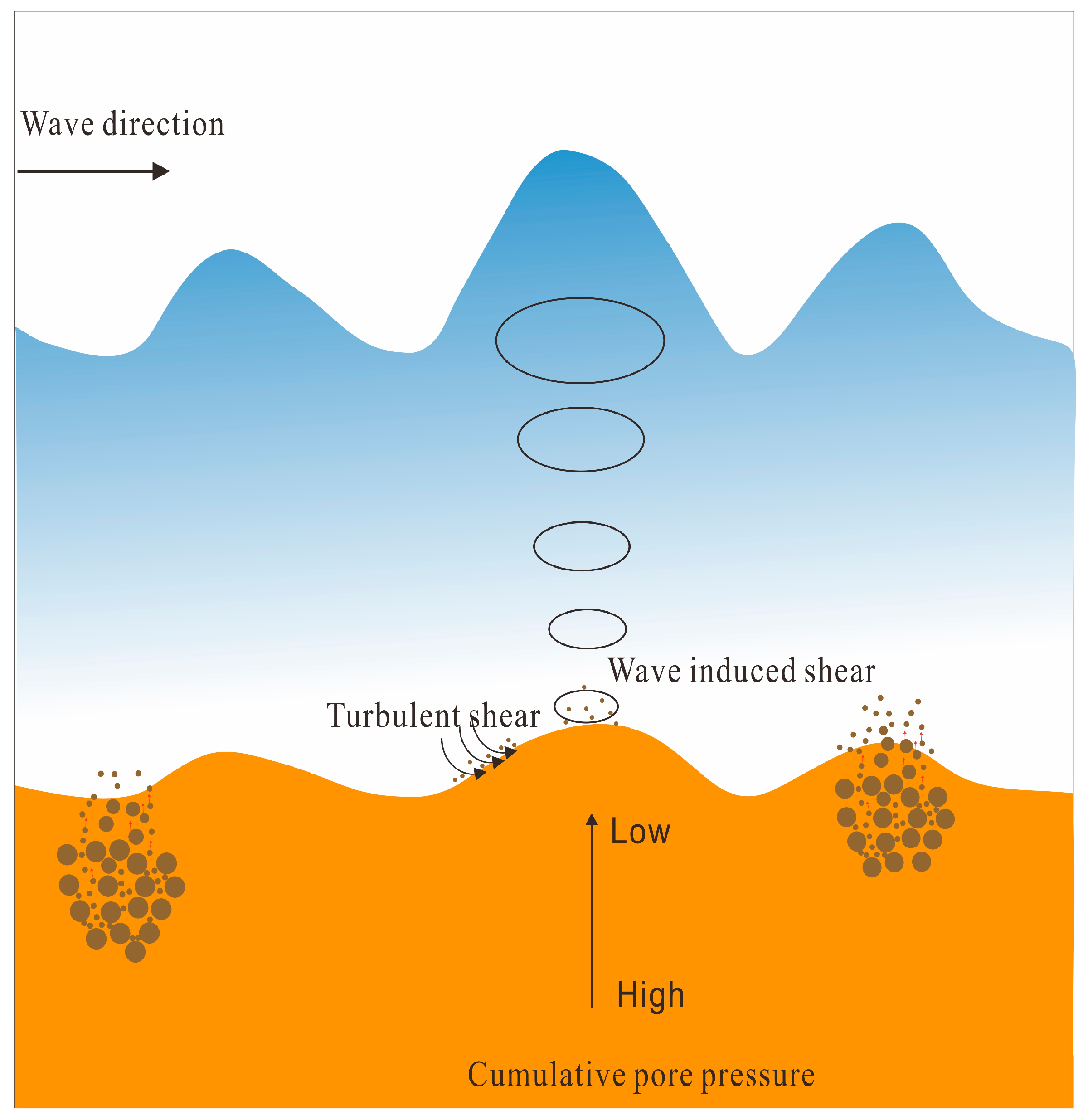
Seabed liquefaction accelerates sediment resuspension in four ways: by reducing the critical shear stress of the soil, by forming seepage channels inside the seabed soil, by forming mud waves and leading to an increase in TKE, and by dissipating excess pore pressure, resulting in the porewater carrying fine-grained sediment upward into the water body, causing an increase in SSC.

References

1. Tzang, S.; Ou, S. Laboratory flume studies on monochromatic wave-fine sandy bed interactions: Part 1. Soil fluidization. Coast. Eng. 2006, 53, 965–982. [Google Scholar] [CrossRef]
2. Wang, H.; Liu, H. Evaluation of storm wave-induced silty seabed instability and geo-hazards: A case study in the Yellow River Delta. Appl. Ocean Res. 2016, 58, 135–145. [Google Scholar] [CrossRef]
3. Xu, G.; Sun, Z.; Fang, W.; Liu, J.; Xu, X.; Lv, C. Release of phosphorus from sediments under wave-induced liquefaction. Water Res. 2018, 144, 503–511. [Google Scholar] [CrossRef] [PubMed]
4. Niu, J.; Xu, J.; Li, G.; Dong, P.; Qiao, L. Swell-dominated sediment re-suspension in a silty coastal seabed. Estuar. Coast. Shelf Sci. 2020, 242, 106845. [Google Scholar] [CrossRef]
5. Zhang, M.; Yu, G.; Andrea, L.R.; Roberto, R. Erodibility of fluidized cohesive sediments in unidirectional open flows. Ocean Eng. 2017, 130, 523–530. [Google Scholar] [CrossRef]
6. Wang, Z.; Luan, M.; Jeng, D.S.; Liu, X. Theoretical analysis of random wave-induced seabed response and liquefaction. Rock Soil Mech. 2008, 29, 2051–2076. [Google Scholar] [CrossRef]
7. Zen, K.; Yamazaki, H. Mechanism of wave-induced liquefaction and densification in seabed. J. Jpn. Soc. Soil Mech. Found. Eng. 1990, 4, 90–104. [Google Scholar] [CrossRef] [Green Version]
8. Wang, L.; Pan, D.; Pan, C.; Hu, J. Experimental investigation on wave-induced response of seabed. Chin. Civil Eng. J. 2007, 40, 101–109. [Google Scholar] [CrossRef]
9. Dey, S.; Sumer, B.M.; Fredsøe, J. Control of scour at vertical circular piles under waves and current. J. Hydraul. Eng. 2006, 132, 270–279. [Google Scholar] [CrossRef]
10. Christiansen, C.; Vølund, G.; Lund-Hansen, L.C.; Bartholdy, J. Wind influence on tidal flat sediment dynamics: Field investiga- tions in the Ho Bugt, Danish Wadden Sea. Mar. Geol. 2006, 235, 75–86. [Google Scholar] [CrossRef]
11. Lou, J.; Ridd, P.V. Wave-current bottom shear stresses and sediment resuspension in Cleveland Bay, Australia. Coast. Eng. 1996, 29, 169–186. [Google Scholar] [CrossRef]
12. Jia, Y.; Zhang, L.; Zheng, J.; Liu, X.; Jeng, D.S.; Shan, H. Effects of wave-induced seabed liquefaction on sediment re-suspension in the Yellow River Delta. Ocean Eng. 2014, 89, 146–156. [Google Scholar] [CrossRef]
13. Liu, X.; Jia, Y.; Zheng, J.; Hou, W.; Zhang, L.; Zhang, L.; Shan, H. Experimental evidence of wave-induced inhomogeneity in the strength of silty seabed sediments: Yellow River Delta, China. Ocean Eng. 2013, 59, 120–128. [Google Scholar] [CrossRef]
14. Zhang, S.; Jia, Y.; Wang, Z.; Wen, M.; Lu, F. Wave flume experiments on the contribution of seabed fluidization to sediment resuspension. Acta Oceanol. Sin. 2018, 37, 80–87. [Google Scholar] [CrossRef]
15. Tzang, S.; Ou, S.; Hsu, T. Laboratory flume studies on monochromatic wave-fine sandy bed interactions Part 2. Sediment suspensions. Coast. Eng. 2009, 56, 230–243. [Google Scholar] [CrossRef]
16. Chiaradonna, A.; d’Onofrio, A.; Bilotta, E. Assessment of post-liquefaction consolidation settlement. Bull. Earthq. Eng. 2019, 17, 5825–5848. [Google Scholar] [CrossRef]
17. Terzaghi, K.; Peck, R.B.; Mesri, G. Soil Mechanics in Engineering Practice; Wiley: New York, NY, USA, 1996. [Google Scholar]
18. Sumer, B.M.; Hatipoglu, F.; Fredsøe, J.; Sumer, S.K. The sequence of sediment behaviour during wave-induced liquefaction. Sedimentology 2006, 53, 611–629. [Google Scholar] [CrossRef]
19. Kramer, S. Geotechnical Earthquake Engineering; Prentice Hall: Hoboken, NJ, USA, 2008. [Google Scholar]
20. Jeng, D.S. Wave-induced seabed instability in front of a breakwater. Ocean Eng. 1997, 24, 887–917. [Google Scholar] [CrossRef]
21. Sumer, B.M.; Kirca, V.; Fredsoe, J. Experimental validation of a mathematical model for seabed liquefaction under waves. Int. J. Offshore Polar Eng. 2012, 22, 133–141. [Google Scholar]
22. Hu, J.; Xu, J.; Niu, J.; Dong, P.; Qin, K. A comparative study of suspended sediment concentrations observed with acoustic and optical methods. Coast. Eng. 2016, 35, 47–57. [Google Scholar] [CrossRef]
23. Grant, W.D.; Madsen, O.S. Combined wave and current interaction with a rough bottom. J. Geophys. Res. Oceans 1979, 84, 1797–1808. [Google Scholar] [CrossRef]
24. Daubechies, I.; Lu, J.; Wu, H.T. Synchrosqueezed wavelet transforms: An empirical mode decomposition-like tool. Appl. Comput. Harmon. Anal. 2011, 30, 243–261. [Google Scholar] [CrossRef] [Green Version]
25. Bian, C.; Liu, Z.; Huang, Y.; Zhao, L.; Jiang, W. On estimating turbulent Reynolds stress in wavy aquatic environment. J. Geophys. Res. 2018, 123, 3060–3071. [Google Scholar] [CrossRef]
26. Lu, Y.; Lueck, R.G. Using a broadband ADCP in a tidal channel. Part II: Turbulence. J. Atmos. Ocean. Technol. 1997, 16, 1568–1579. [Google Scholar] [CrossRef]
27. Zen, K.; Yamazaki, H. Field observation and analysis of wave-induced liquefaction in seabed. Soils Found. 1991, 4, 161–179. [Google Scholar] [CrossRef] [Green Version]
28. Xu, X.; Xu, G.; Yang, J.; Xu, Z.; Ren, Y. Field observation of the wave-induced pore pressure response in a silty soil seabed. Geo-Mar. Lett. 2021, 41, 13. [Google Scholar] [CrossRef]
29. Song, Y.; Sun, Y.; Du, X.; Li, S. The pore pressure response characteristics and process of the silt in the Yellow River Delta under wave action. Adv. Mar. Sci. 2019, 37, 452–461. [Google Scholar] [CrossRef]
30. Liu, X.; Jia, Y.; Zheng, J. In situ experiment of wave-induced excess pore pressure in the seabed sediment in Yellow River estuary. Rock Soil Mech. 2015, 36, 3055–3062. [Google Scholar] [CrossRef]
31. Prior, D.B.; Suhayda, J.N.; Lu, N.Z.; Bornhold, B.D.; Keller, G.H.; Wiseman, W.J.; Wright, L.D.; Yang, Z.S. Storm wave reactivation of a submarine landslide. Nature 1989, 341, 47–50. [Google Scholar] [CrossRef]
32. Wen, M.; Jia, Y.; Wang, Z.; Zhang, S.; Shan, H. Wave flume experiments on dynamics of the bottom boundary layer in silty seabed. Acta Oceanol. Sin. 2020, 39, 96–104. [Google Scholar] [CrossRef]
33. Xu, G. Study on the Landslide of Gentle Slope Silty Seabed under Wave—A Case of Yellow River Subaqueous Delta. Ph.D. Thesis, Ocean University of China, Qingdao, China, 2006. [Google Scholar] [CrossRef]
Figure 1. Layout of the experimental flume and particle size distribution curve of the experimental soil.: (a) layout of the experimental flume; (b) layout of measuring instruments and sensors; (c) particle size distribution curve of the experimental soil. Note: d50 is the average particle size of the soil and CC is the percentage of clayey particles in the soil.
Jmse 10 00437 g001
Figure 2. Correlation relationship between turbidity and SSC derived from calibration experiments.
Jmse 10 00437 g002
Figure 3. Time-series of random waves, excess pore pressure, and cumulative pore pressure during the experiment process: (a) time-series of random waves (blue curve) and excess pore pressure at a depth of 10 cm (red curve); (b) time-series of random waves (blue curve) and excess pore pressure at different depths (other colors, detailed view); (c) cumulative pore pressure at different depths over time, with the dashed line indicating the time taken to reach the first crest at distinct depths.
Jmse 10 00437 g003
Figure 4. Time-series of random waves and excess pore pressure at various depths in experiment IV-2: the shaded bar shows σ 0   ,   the   initial mean normal effective stress of the seabed; and the white curve shows cumulative pore pressure.
Jmse 10 00437 g004
Figure 5. Excess pore pressure response for liquefied seabed impacted by random waves in Experiment IV-2 (detailed view): blue curve—random waves; orange curve—excess pore pressure response at 5 cm below the seabed; black curve—excess pore pressure response at 30 cm below the seabed;   σ 0   —initial mean normal effective stress of the seabed.
Jmse 10 00437 g005
Figure 6. Variation on the water–soil interface during a single wave cycle. (ad) is the photograph at 512, 512.5, 513 and 513.5 s after the wave action in experiments IV-2, respectively.
Jmse 10 00437 g006
Figure 7. Fluctuation of mud waves along with water waves through time: blue curve—random waves; black curve—seabed interface.
Jmse 10 00437 g007
Figure 8. Response of SSC impacted by the waves: (a,b) represent experiments II-3 and II-4, with effective wave heights of 16 cm and 18 cm, respectively, depicting the SSC response of nonliquefied seabed; (c,d) represent experiments IV-2 and IV-3, with effective wave heights of 16 cm and 18 cm, respectively, depicting the SSC response of liquefied seabed.
Jmse 10 00437 g008
Figure 9. Change in SSC with time (at 5 cm above the seabed): red line—liquefied seabed (Experiment IV-2); and black line—non-liquefied seabed (Experiment II-3).
Jmse 10 00437 g009
Figure 10. Relationship between SSC (at 5 cm above the seabed) and wave-induced shear stress in the (a) non-liquefied and (b) liquefied states; the red curve is SSC and the black curve is wave-induced shear stress, τ w .
Jmse 10 00437 g010
Figure 11. Changes through time in response to wave condition IV-2: (a) random wave elevation, (b) excess pore pressure (z = 5 cm), (c) SSC (at 5 cm above the seabed), and (d) the measured water flow velocity at 5 cm above the seabed.
Jmse 10 00437 g011
Figure 12. Time-variation of the turbulent velocity, TKE, and SSC (at 2 cm above the seabed): (a,b) are the nonliquefied state and the initial stage of the liquefied state, respectively, where 𝑢t, v’t, and w’t represent the longitudinal, transverse, and vertical components of the turbulence, and TKE is the turbulent kinetic energy; (c,d) represent the later stages of liquefaction.
Jmse 10 00437 g012
Figure 13. Sketch map showing the dynamic response of liquefied soil to random waves.
Jmse 10 00437 g013